Abstract
The paper deals with the connection between the issue of rectification of the structural system and the corresponding experimental and related statistical analysis of stresses. The solution was demonstrated in the example of replacing the aboveground gas pipeline with an underground solution. During the implementation of landscaping for the underground solution, there was a risk of damage to the existing structure. Due to the specific problems in stress analysis based on strain gauge measurements, especially with regard to the narrow range of gas pressure as the primary input quantity, the obtained data had to be subjected to complex statistical procedures. Several linear and non-linear regression models were compiled and subjected to normality, homoscedasticity, and autocorrelation tests. The data obtained in this manner ruled out the possibility of limited state occurrence on the existing structure and, in conjunction with other information, enabled the successful completion of the rectification process to its current form. The scientific added value of the contribution should be the demonstration of procedure methodology and relatively unconventional use of regression and correlation analysis methods and means in the technical field for stress analysis in solving engineering practice problems.
1. Introduction
The transport of gaseous and liquid media such as water, oil, steam, or natural gas is carried out very efficiently through pipe systems such as water, oil, steam, and gas pipelines. Part of such pipe systems are or can also be complex technological units, mainly compressor and pumping stations, border transfer stations, connection and distribution nodes, underground storage, etc.
All technical equipment for the transport of media, especially oil and gas, are of strategic nature, and their failure often leads to fatal consequences, economic damage, loss of life, etc. Therefore, constant monitoring of all structural elements of the transport system for the possible occurrence of a limit state is necessary, as well as their continuous intensification and rectification, if needed.
The transport infrastructure facilities for gaseous and liquid media must be designed and constructed to meet certain requirements, mainly:
- Suitability for the respective use with regard to the expected lifetime and costs incurred and with an acceptable probability;
- Resistance to operational loads and other influences acting during the installation and operation of the pipeline with acceptable reliability;
- Resistance to limit state formation.
- Potential damage to pipelines and other related equipment must be prevented or at least limited by using appropriate means, e.g.;
- By completely eliminating or at least significantly reducing all risks;
- By designing the shape of the structure in a way, that reduces the sensitivity to random risk.
In order to detect and prevent the emergence of a limit state in the elements of the gas pipeline transport system, it is necessary to ensure a set of activities, primarily the following:
- Monitoring of the occurrence of the limit state, especially the related service life of structural elements of pipelines and yard piping of compressor stations and its prediction. In such cases, the correct assessment and prediction of the remaining service life and strength of yard piping of the compressor stations after several years of continuous operation is a particular issue [1,2,3,4,5,6,7].
- Verification of stability or changes in material properties of structural elements of pipelines and yard piping of compressor stations as a result of degradation processes and the potential impact of these changes on the emergence of a limit state. Special attention is paid to the possible degradation of welds and the material itself [8,9].
- Rectification of older pipeline bridges and other temporary or insufficient technical solutions. In such cases, in particular, the possibility for the construction of earthworks related to the emerging solution to have a negative impact on the original solution may be a specific issue [10].
- Monitoring corrosion-damaged pipelines and their rectification, e.g., using pressurized sleeve technology. In such cases, the development of a pressurized sleeve and a suitable polymer filling material is a very special technological and design problem [11].
All the analyses mentioned, which are related to the rectification, assessment of the condition and prediction of the service life of pipeline system structures, included short-term or long-term static or dynamic strain gauge measurements, subsequent static or dynamic stress analysis, in most cases, some form of statistical data processing was also used. Experimental and statistical methods were also applied in the analysis of mechanical, stress, deformation, fatigue, energy quantities, and other quantities, mainly for assessing the degradation of structural materials of pipeline systems.
The contribution deals with the issue of structural system rectification, corresponding experimental analysis, and related statistical analysis of stresses. The mentioned combination of the experimental analysis of stresses, obtained by strain gauge measurement with the creation of regression models of stress dependencies, with the subsequent validation of these models by correlation analysis, is relatively rare in the available literature. Such statistical solutions are usually applied in the economic field, and their application in the technical field is relatively infrequent. In the available literature, it is quite difficult to find newer or more relevant sources that cover this topic, especially with emphases on a rather unconventional combination of the use of regression and correlation analysis methods and means in stress analysis with the requirement to solve the issues of structures rectification in technical engineering practice.
The mentioned issue is demonstrated in the example of rectification of the overhead line of the transit gas pipeline by replacing it with an underground solution. In the process of preparatory earthworks for the new solution, strong vibrations occurred in the immediate vicinity of the original solution during the hammering of sheet piles; it was thus necessary to analyse possible negative impacts on the original solution.
1.1. Gas Pipeline System on the Territory of the Slovak Republic
The gas pipeline system for transporting natural gas on the territory of the Slovak Republic in the east-west direction is the transportation system of the company Eustream; it is a system of several parallel pipelines with a diameter of 1200 and 1400 mm with a total length of more than 2200 km, with a maximum operating pressure of 7.35 MPa, continuously built since 1967 (Figure 1 and Figure 2). The system has a distinct transit character and, for strategic reasons, is technically and technologically adapted for both directions of gas flow [12,13].
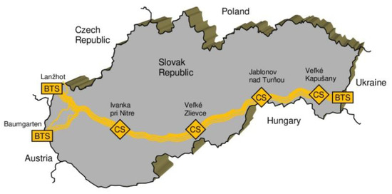
Figure 1.
Scheme of the Eustream transport network on the territory of the Slovak Republic, where: CS—compressor station, BTS—border transfer station.

Figure 2.
Part of parallel underground lines of the Eustream transport network recognizable on a satellite image.
1.2. Requirement of Rectification of Older Technical Solutions
A serious structural and technological problem in the design and implementation of pipeline systems is overcoming various terrain obstacles, especially watercourses. The original bridging of larger rivers with gas pipelines on the territory of the former Czechoslovakia Republic, and later in the Slovak Republic, was solved with load-bearing structures, i.e., bridging with pipeline bridges. The chosen concepts were based on the material and technological possibilities of the time. Three main methods or the structural solutions of pipeline bridges were used: truss three-span straight continuous beam, truss three-jointed arch (Figure 3a), and the self-supporting pipe (arch) (Figure 3b) [12,14].

Figure 3.
(a) Truss three-jointed arch; (b) Self-supporting pipe.
In the later period, transport lines were, in most cases, built using a more modern approach to watercourse crossing designs by pulling crossings under the watercourses. As a result of their overall design and easy accessibility, the existing older transport infrastructure pipelines are generally the most vulnerable objects in the entire transport system. This applies particularly to situations of threat in the event of war conflicts, and terrorist attacks, but also as a result of natural disasters. Figure 4 shows the condition of the bridge supporting structure after its destruction during the 1974 floods on the Slaná River in the Slovak Republic.

Figure 4.
Destruction of the supporting structure of the bridge during the floods in 1974 on the Slaná River.
Therefore, in the current period, safety, technological, economic, and strategic reasons have required the application of the rectification concept, the essence of which is the gradual reconstruction of existing aboveground river crossings and their replacement with underground solutions. Part of the concept adopted is to take care of the condition of the pipelines themselves as well as the condition of compressor stations, particularly with regard to the possibility of corrosion damage or more serious limit states, such as the risk of fatigue failure.
1.3. The Problem of the Current Coexistence of the Old and New Bridge under Construction
During the reconstruction of the old aboveground and the implementation of new underground solutions, a problem arose in the partial coexistence of both solutions. In certain cases, a new solution, i.e., the pipeline under the river flow, due to the geographical situation, was implemented in the immediate vicinity of the attachment of the support structure of the aboveground solution or near the inlet of its pipeline into the ground. The new solution also required significant landscaping. Considering the overall layout solution and in order to keep the cost of the pipeline relocation as low as possible, it was necessary to carry out these landscaping works near the original pipeline bridges; it was possible to assume that complex landscaping in the vicinity of aging pipeline bridges could have an adverse effect on their structure, i.e., the damage it, e.g., shocks and vibrations arising from the hammering of sheet piles during the creation of sheet pile walls.
In this context, it was necessary to perform an analysis of the reaction or responses of the old pipeline bridges as a result of technological construction activities during landscaping. Consequently, a series of dynamic strain gauge measurements were performed on gas pipelines during simulated construction modifications. In particular, the deformation and change of mechanical stresses in the pipe elements during the transmission of vibrations from construction machines were investigated. Strain gauge measurements were performed at selected locations on the pipe surface. At the same time, strain gauge measurements were also carried out during the pressure change in the pipeline, especially at its maximum load.
The object of analysis or of the strain gauge measurements was the DN 1400 pipeline crossing of the fourth line of the Transit gas pipeline over the Laborec river in the Slovak Republic. The actual bridging was implemented by a double-arch self-supporting pipe, partially shown in Figure 5a, with a view in the direction of gas flow. The pipeline was equipped with a monitoring and technological bridge on one side.
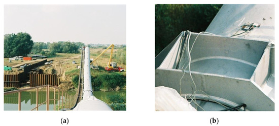
Figure 5.
(a) View on the self-supporting pipeline in the direction of gas flow; (b) Detail of the applied strain gauges at the foundation footing.
2. Materials and Methods
2.1. Experimental Measurements of Stresses in the Pipe Wall
During the implementation of the experiment, two series of strain gauge measurements in three locations on the pipeline were considered in order to determine the stress increments in the pipe wall on the inlet side of the pipeline:
- At the pipe inlet near the foundation foot (called the racket) on the right bank of the river with detail of the strain gauges used shown in Figure 5b; these strain gauges were grouped into two groups, labelled G2 and G3 in the diagram in Figure 6; their purpose was to measure, in the monitoring mode, the response in the pipeline caused by dynamic shocks during the hammering of sheet piles in the immediate vicinity of the foundation footing;
 Figure 6. Scheme of the placement of strain gauges on pipes in three groups, G1 to G3.
 - At all locations G2 and G3 from the previous measurement mode, and additionally at the top of the pipeline arch above the river with a group of strain gauges G1 (Figure 6), in the mode of measuring and monitoring the response in the pipeline during changes in gas pressure in the pipeline.
The measuring points or locations for the application of electrical strain gauges were chosen with respect to the results of previous numerical and experimental analyses, as well as considering the possible effect of material bifurcation on the stress in the pipe wall. Rectangular strain gauge rosettes with three measuring grids were used as measuring sensors. The strain gauge measurement chains were used for the dynamic measurement mode in the configuration shown in Figure 7 and for the static measurement mode.

Figure 7.
Configuration of the strain gauge measuring chain used for dynamic measurement.
2.2. Data Obtained by Experiment and Their Formal Interpretation
For the mode of measuring and monitoring the response in the pipeline caused by dynamic shocks during the sheet pile hammering, the position of the sensors was chosen so that the response of the system to the dynamic excitation was sensed at the pipeline bridge as close as possible to its foot. Several implementations were carried out in this dynamic strain gauge mode, each lasting approximately 1 min. The first part of the measurements was carried out in a rest state without the effects of shocks during impacts. The second part of the measurements was carried out while hammering the sheet piles. The measurements at rest were carried out in order to distinguish the effects of the stress increase caused by the hammering of sheet piles from other effects. The measured values of the strains, later converted to principal normal stresses, were statistically processed in the post-processing by means of regression and correlation analysis in the Matlab software environment. Partial results from these implementations are shown in Figure 8 and Figure 9.

Figure 8.
Time dependence of stresses expressed from measured strains.
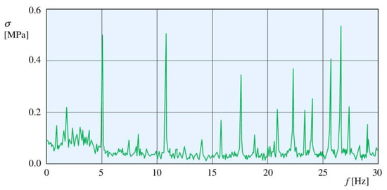
Figure 9.
Amplitude spectrum of strains converted to uniaxial tension.
Figure 8 shows the time dependence of the increments of the principal normal stresses in the circumferential direction, expressed on the basis of the measured strains. Figure 9 shows the amplitude spectrum of strain increments, which for ease of interpretation, is converted to the principal normal stress of the uniaxial stress according to Hooke’s law relation.
The second objective of the series of measurements was to determine the increments of circumferential and axial normal stresses Δσt and Δσm in the pipe wall caused by the change in the pressure Δp of the transported gas at time t or Δt. Since the absolute values of these stresses from the gas pressure in the pipeline are superimposed on the stresses created by the sheet pile hammering shocks, they could potentially cause a limit state to occur. Therefore, for the overall assessment of the resistance of the existing bridge to the effects of construction operations, data from both modes of measurement were necessary.
The basis for the calculation or determination of pipeline gas pressure at the place of strain gauge measurements was information about the pressures supplied by the gas pipeline operator from the control post, e.g., as shown in Figure 10. However, as the distance from the checkpoint increases, the pressure decreases. Therefore, the supplied data were converted to pressure values at the measurement place by special procedures listed in [10]. When the gas pressure decreases, the specific volume of the gas increases and at the same time, the speed increases. Simultaneously, due to friction, energy is also lost, and the temperature of the pipeline increases, which at the time and place of measurement reached a value in the range of 35.2 °C to 40.8 °C.

Figure 10.
Values of pressures p [MPa] with a display coefficient of 0.08 in the pipeline in a time range of approximately 9 h were obtained from the pipeline operator control station.
2.2.1. Statistical Analysis of Experimentally Obtained Results
There were complications during the experiment in determining stress increments or drops Δσt and Δσm at the measurement point G1 to G3 due to pressure change Δp. For technological and operational reasons, the pressure in the pipe p at time t could not be changed in the overall range from 0 to pmax, but only in a relatively small range of 5.67 MPa to 6.32 MPa. In this way, discrete values were obtained experimentally in the form of n1 ordered pairs [pi, ti], n2 ordered pairs [Δσti, Δpi] and n2 ordered pairs [Δσmi, Δpi], for n1 = 18 and n2 = 20. The stresses Δσti and Δσmi were recalculated from the data measured with strain gauge rosettes. Considering the type, nature, and character of the obtained results and with regard to their objective interpretation, it was appropriate to process them by statistical means, in particular by regression and correlation analysis methods.
From the point of view of statistics, the specified ordered pairs n1 and n2 form the multivariate statistical files. The question of finding, investigating, and evaluating the connection or dependence between two quantitative statistical features is addressed by statistics using regression and correlation analysis. Regression analysis addresses the task of detecting the dependence and expressing it by mathematical means, i.e., the regression function. In an extreme case, it solves whether there is any dependence or connection at all. Correlation analysis addresses the task of determining the tightness of dependence or the degree of intensity with which the dependence being regressed manifests itself among the various interfering secondary factors, or assesses the degree of correctness of the regression analysis performed.
2.2.2. Regression Analysis of Experimentally Obtained Results
The entire regression analysis procedure can be divided into three points:
- Selection of the appropriate regression model;
- Determination or estimation of relevant coefficients;
- Description of the applied regression model by examining the residuals.
Therefore, the first task is the choice of a suitable regression model. Basically, it is a proposal of the mutual behaviour of the investigated quantities. Through the points of the ordered pairs, it is necessary to lead a certain curve, analytically represented by a certain mathematical function, which will represent them as best as possible. The simplest regression model is a linear model, represented by a linear function, a polynomial of the first degree. In more complex cases of interdependence, one of the non-linear models can be applied; it can be a quadratic (parabolic) model prescribed by a second-degree polynomial or, in more complex cases of dependence, a cubic model prescribed by a third-degree polynomial. Other nonlinear models used are hyperbolic, logarithmic, exponential, power, etc., prescribed by relevant functional dependencies. Based on the knowledge and experience acquired, the solver then chooses one or some of them. The degree of correctness is subsequently verified by means of appropriate tests and means of correlation analysis.
In this case, it was a matter of determining three regression dependencies: p = f(t) (RD1), Δσt = f(Δp) (RD2) and Δσm = f(Δp) (RD3). In searching for them, a design procedure of several models was chosen, and the most appropriate one was selected based on their evaluation. For each of them, three models were chosen: linear, quadratic and cubic, represented by polynomials of the first degree, second degree, and third degree.
For example, for RD1, the proposed cubic regression model (regression curve, line) has the analytical form:
where βj for j = 0, 1, … s, (where s is the degree of the polynomial) are the unknown values of the parameters of the regression curve. Nevertheless, during the calculation, the so-called smoothing regression line will be applied, expressed in the form:
where is the balanced (theoretical, calculated) value of the real variable and for j = 0, 1, … s, j = 0, 1, … s, are point estimates (parameters) that should approximate as accurately as possible, i.e., approximately replace unknown parameters (regression coefficients) βj. A point estimate means an estimate by a single number, as opposed to an interval estimate, which is an estimate by a number interval.
The second step of regression analysis is parameter estimation. Point estimates of the unknown parameters βj of the regression line are most often obtained from the analysed data by the method of least squares (MLS). The purpose of applying this method is to minimize errors arising as a result of differences between the calculated, i.e., theoretical, and established (empirical) values, e.g., measured values of the dependent variable; these differences can acquire both positive and negative values. Therefore, they are squared, and their sums are expressed, referred to as the residual error sum of squares or the sum of square errors SSE. SSE represents the sum of squared deviations of empirical and theoretical values of the dependent variable. One such considered square is graphically marked in Figure 11 for one of the values of the third degree polynomial for RD1. The size of the square side represents the residual , as the difference between the empirical and theoretical value of the investigated variable:
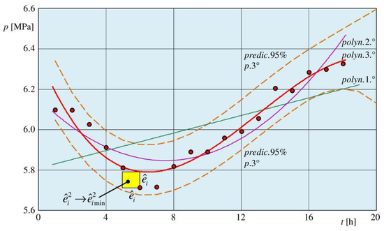
Figure 11.
Comparison of three proposed polynomial regression models for the dependence p = f(t) and marking of the 95% prediction interval for the applied polynomial model of the third degree.
It is true and obvious that the better the model, the larger the sum of squares of the model and the smaller the residual sum of squares. Conversely, an inappropriate model implies a large value of the residual sum of squares compared to the model sum of squares. The SSR quantity is the theoretical or regression sum of squares as the sum of the squares of the deviations of the theoretical values from the average of the empirical (measured) values. By summing the SSE and SSR quantities, it is possible to obtain the total sum of squares SST as the sum of the squares of the deviations of the empirical values depending on the variable from the average of the empirical values. In general, the estimates obtained by applying the MLS method are considered objective, with minimal variance.
Point estimates obtained by the MLS method are random variables with a normal distribution. Therefore, from the point of view of the accuracy and objectivity of the solution, it is also appropriate to express the confidence (prediction) interval for each of the parameters , representing the interval of all permissible values of the estimated parameters.
Table 1 shows a part of the calculated values of point estimates and the corresponding confidence prediction intervals for RD1, RD2, and RD3.

Table 1.
Parameters of applied polynomial models of the first degree of individual regression dependencies.
For comparison, the courses of polynomial dependencies of the three proposed polynomial regression models for RD1 p = f(t) are plotted (see Figure 11), using the data from Table 2.
Table 2.
Parameters of applied polynomial models of the second and third degree of individual regression dependencies.
Figure 12 shows the values of the residuals for the pressure values against the actual obtained p values for the applied or chosen polynomial model of the third degree RD1 p = f(t). Figure 13 shows the applied or chosen polynomial regression models of the second degree for RD2 Δσt = f(Δp) and for RD3 Δσm = f(Δp), using data from Table 2.

Figure 12.
Graphical representation of the residuals for the pressure values against the actual obtained p values for the applied polynomial model of the third degree of dependence p = f(t).

Figure 13.
Applied polynomial regression models of the second degree for the dependencies Δσt = f(Δp) and Δσm = f(Δp) and marking of their 95% prediction interval.
2.2.3. Correlation Analysis and Regression Dependencies Testing
In terms of objectivity, validity, and interpretation of the regression dependencies and related point estimates obtained, it is necessary to test them with relevant hypotheses; it is also desirable to determine confidence intervals for these parameters. An important task of the regression model of the sought dependence is also the prediction of new values of the investigated quantity for the prediction interval. In general, the prediction interval is wider than the confidence interval. Figure 11 and Figure 13 show the 95% prediction intervals of applied RD 1, 2 and 3.
In general, hypothesis testing will be understood as a procedure in which, based on the relevant analysis, a decision is made whether, at the selected level of significance α, i.e., with the selected reliability 1-α, or 100-α [%], the given hypothesis will or will not be rejected. In case of rejection, the opposite hypothesis is accepted. Thus, in testing, the principle of two opposing hypotheses is chosen, one of which asserts something, and the other rejects that assertion. Most of the time, the so-called null hypothesis H0 is chosen as the primary one, consisting of a statement that is assumed considering the circumstances; it is opposed by the so-called alternative hypothesis H1, which is accepted after H0 is rejected. The significance level α = 0.05 is chosen if the risk of error is sufficiently small. In some cases, if incorrect acceptance of the alternative hypothesis H1 could have some serious consequences, a lower level of α = 0.01 is chosen.
To evaluate a certain RD, the selective residual variance, also called mean squared error MSE, obtained from SSE is first applied. MSE represents a point or unbiased estimate of the interval variance σ2; it expresses the measure of how, on average, the theoretically obtained value differs from its empirical equivalent, that is, how the values of the analysed variable are scattered around the regression function. The point estimate of the standard deviation σ is the root mean squared error RMSE as the square root of the MSE [15,16,17,18].
Using the SSE, SSR, and SST values, it is then possible to express the R-squared or coefficient of determination R2. R2 reaches values in the range of 0 to 1. For values close to 1, especially with a sufficiently large set of values, it is possible to infer the mutual dependence of two quantities and a well-chosen regression function. On the contrary, values approaching zero indicate a weak interdependence of the two quantities or an inappropriately chosen regression function. The disadvantage of the R2 parameter is that it generally does not have the property of symmetry. This means that when measuring the closeness of the dependence of two quantities, the closeness of the first quantity to the second is or can be different from the closeness of the second quantity to the first. Another disadvantage of the R2 parameter is that for small sample ranges, this estimate is biased and overestimates the fit of the regression model. In such a case, an unbiased estimate of the coefficient of determination, the so-called modified or corrected coefficient of determination—the adjusted R-square R*2—is then applied.
A number of sophisticated statistical tests are available to test the reliability and validity of the proposed regression models and specific RD in more detail, to investigate their specific properties, and to detect even less obvious shortcomings. Such tests are e.g., normality test, homoscedasticity test, autocorrelation test, etc. The basic principle of these tests is the application of two hypotheses, the null H0 and the alternative H1. Based on the relevant test statistic Vstat as a certain statistical quantity belonging to the given test and its comparison with its critical value Vstatcrit, for the relevant level of significance α, a decision is then made to accept or reject that hypothesis. Usually, if the relevant test statistic exceeds the critical value, the null hypothesis H0 is rejected, and the alternative hypothesis H1 is accepted. The so-called p-value has a similar application if it is part of the output of the respective test. This, in turn, is compared with the corresponding level of significance α, again for the acceptance or rejection of a particular hypothesis. The p-value is the probability of obtaining a more extreme result if the null hypothesis is true. If the p-value is low (e.g., <=0.05), the alternative hypothesis will be more likely [19,20,21,22,23].
Table 3 shows basic data of the three test procedures applied in the analysis, specifying the tested property, the null hypothesis H0 and the alternative hypothesis H1.
Table 3.
Basic data of the three test procedures applied.
Normality means a normal distribution of residuals. Thus, the Anderson–Darling test is used to verify the fulfilment of this property.
Homoscedasticity will be understood as the finite and constant variance σ2 of random components and thus also of residuals or that the variance does not change as the independent variable changes. Otherwise, it will be heteroscedasticity. Verification of this property can be realized by the Goldfeld–Quandt test.
Autocorrelation will be understood as the state when random components influence each other or the assumption of non-correlation is not met, i.e., independence of random errors, and they show some form of systematic behaviour. The Durbin-Watson test can be used to verify this property. The values of the DW test statistic Vstat range from 0 and 4. A value of 0 means that there is positive autocorrelation between random components, and a value of 4 means negative autocorrelation. A value of 2 indicates that the random components are independent and that there is no autocorrelation between them. The permissible interval for non-correlation is wider, of course, ranging from 1.4 to 2.6. If the autocorrelation is very strong (significant), i.e., there is a high dependence between random components, an inappropriate model has probably been chosen. Significant autocorrelation may also be caused by a violation of the linearity assumption if such a linear model was assumed [15,16,17,18].
In Table 4 and Table 5, the selected correlation parameters and results of test procedures used in this analysis are listed. In Table 5, for clarity, the parameters and results of the test procedures of only the selected polynomial models, namely third degree for RD1, and second degree for RD2 and RD3, are presented.
Table 4.
Parameters of correlation analyses of proposed polynomial models of individual regression dependencies p = f(t), Δσt = f(Δp) and Δσm = f(Δp).
Table 5.
Parameters of correlation analyses of applied polynomial models of individual regression dependencies p = f(t), Δσt = f(Δp) and Δσm = f(Δp).
All stated values and dependencies were obtained directly in the environment of the MATLAB and MS Excel software systems or indirectly—with the support of these environments.
3. Results and Discussion
The evaluation of strain gauge measurements and all related analyses showed that the stress increments detected on the pipeline just before entering the support foot were negligible during the sheet pile hammering. The recorded stress changes were comparable to the measurement made in the resting state and did not exceed the value of ±2 to 3 MPa.
In the case of monitoring the response of the pipeline to pressure changes in it, it was necessary to understand the stresses detected by the measurement as increments of their values Δσ, which are related to increments of pressure Δp compared to its reference value at pref = 6,0972 MPa. The largest stress increases were recorded by the strain gauge located at the top of the arch above the river. Based on the correlation analyses performed on the resulting regression dependences of Δσt and Δσm on Δp, it was found that from a statistical point of view, the quadratic polynomial model is slightly more representative than the linear polynomial model.
However, this was particularly true for a range of measured values. In case of need for extrapolation of these dependencies and reverse reconstruction of the total values of stresses σt and σm and their dependence on the input (primary) quantity, i.e., pressure p in its wide range of 0 to 6 or 7 MPa, was required, the quadratic models provided unrealistic or distorted results. Therefore, paradoxically—a slightly less representative from a statistical point of view, but far more realistic from a technical point of view—a linear model was chosen for extrapolation purposes.
The increments of shear stresses in the pipe wall in the monitored locations were small, and the calculated values are smaller or comparable to the resolution or tolerance of the measuring chain; it is, therefore, possible to assume that the directions of the principal normal stresses are identical to the circumferential and axial directions of the pipe; these small values of shear stress increments correspond to a lower value of both the correlation coefficient and the coefficient of determination; it follows that with small shear deformations, the influence of measurement inaccuracy, given by the resolution of the measurement chain as well as the physical nature of the measurement method, is more pronounced.
This model showed that the increase in pressure Δp by 1 MPa corresponded to the approximate increases in normal stress in the circumferential direction Δσt = 61.5 MPa and in the axial direction Δσm = 46.0 MPa. The analysis showed that this pair of stresses is also a pair of principal stresses. Therefore, they could also be used to determine the corresponding unit value of the equivalent stress σeqVM according to the Von Mises theory at a level of 55.4 MPa. Further, with the application of this linear regression model for the reference value of pressure at the level of pref = 6.0972 MPa, it was then possible to further express the corresponding absolute values of the stresses σt and σm at the level of 374 and 280 MPa and the corresponding level of the equivalent stress σeqVM at the level of 337 MPa.
At the same time, for stress increments above 10 MPa, a significant dependence of their values on the pressure in the pipeline was observed. Moreover, from a mutual comparison of the curves of stress increments Δσt and Δσm and at the same time against pressure changes Δp from the curves in Figure 13, a weak geometric nonlinearity of the pipeline at the measurement point can be assumed. It is concluded that this could probably be caused by a different change in the pipe diameters in the horizontal and vertical direction by changing the circular cross-section to an elliptical one due to the effect of the pressure in the pipe.
Taking into account the maximum stress increments of 2–3 MPa caused by shocks during construction work to stresses from operating pressures p, values of 377 and 283 MPa were obtained for the stresses σt and σm with the corresponding equivalent stress σeqVM at the level of 340 MPa. The structural material of the original structure from the early 1970s corresponded with its material characteristics to today’s L485ME EN ISO 3183 steel with stress values—onventional yield strength Rp0.2 at least 490 MPa and conventional ultimate strength Rm at least 550 MPa. The analyses carried out clearly showed that the construction works carried out in connection with the construction of the future river crossing had no impact on the condition of the existing crossing and on the possible emergence of an undesirable limit state.
Further, the results of the mentioned analyses eventually allowed for the successful rectification of the bridging and contributed to the gradual replacement of bridging P1 (self-supporting pipe - arch) and later also P2 (truss three-jointed arch), as can be seen in Figure 14a by the underground solution of the river crossing. The current situation at the site of the former overhead bridges P1 and P2, therefore, has the form according to the satellite image in Figure 14b [24].
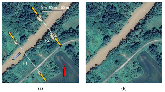
Figure 14.
(a) Original gas pipeline bridges P1 and P2 over the Laborec river, (b) Current underground solution for crossing all 4 branches of the gas pipeline (the blue arrow indicates the direction of water flow, the yellow arrows indicate the direction of gas flow in the pipe, and the red arrow indicates north).
In the case of solving similar problems of other types of structures, it is difficult to accurately estimate the resulting effect of the action. Each case would have to be considered individually in view of its particularities. The type of construction of the original solution would play an important role here. Other influencing factors here could be the distance between the original and the new solution, the type and intensity of preparatory construction work, etc. However, it is possible to express an assumption or hypothesis that in the case of structures where the pipe is not self-supporting but is placed on a supporting structure, the resulting effect is smaller.
4. Conclusions
Oil and gas pipeline systems are part of technological units intended for the long-distance transport of gaseous and liquid media. On their routes, they have to overcome various terrain obstacles, which are often watercourses. At the time of the construction of these pipeline systems, several types of structural solutions for aboveground pipeline bridges were applied in the conditions of former Czechoslovakia, and later in the Slovak Republic. The chosen design and technological concepts were based on the material, economic and technological possibilities of the relevant time. Nonetheless, the necessity of their gradual rectification, especially for operational, security, technological, economic, and strategic reasons and the application of underground solutions in practice sometimes led to the temporary coexistence of the original and emerging solutions. Furthermore, during the implementation of landscaping for the new solution, there was often a potential risk of a negative impact on the structural elements of the existing solution. In particular, there was a risk of unwanted shocks and vibrations during the hammering of sheet piles during the creation of sheet pile walls. The mentioned problem was solved by experimental analysis of stresses within the response of structures by applying static and dynamic strain gauge measurements. Considering the specific problems in this measurement, especially the very narrow range of the gas pressure in the pipeline as the input primary variable, the measured data had to be subjected to complex statistical analyses in order to objectify the conclusions; these included the creation of several linear and nonlinear regression models, which were subsequently subjected to regression analyses by applying relevant testing procedures, especially of normality, homoscedasticity, and autocorrelation testing. However, it is necessary to emphasize that the entire evaluation process was significantly subjectively influenced by choice of the regression model when the dilemma of choosing between a more mathematically or technically optimal regression model was mainly resolved. The obtained data and the related stress analyses did not confirm the unwanted effects of the preparatory earthworks and related activities and ruled out the possibility of the occurrence of a limit state on the existing bridge structure; these conclusions, together with information from further analyses, then contributed to the successful completion of the rectification process in its current form. The scientific added value of the contribution should be the demonstration of the procedure methodology and relatively unconventional use of regression and correlation analysis methods and means in the technical field for stress analysis in solving engineering practice problems.
Author Contributions
Conceptualization, P.F. and P.S.; methodology, P.F. and P.S.; software, D.H.; validation, P.F., P.S., I.D. and P.Š.; formal analysis, P.F., P.S., I.D. and P.Š.; investigation, P.S. and I.D.; resources, P.F., P.S., I.D., D.H. and P.Š.; data curation, P.S. and I.D.; writing—original draft preparation, I.D. and D.H.; writing—review and editing, P.S., I.D. and P.Š.; visualization, P.S., I.D. and D.H.; supervision, P.F.; project administration, P.F.; funding acquisition, P.F. All authors have read and agreed to the published version of the manuscript.
Funding
This research was funded by VEGA No. 1/0500/20, VEGA No. 1/0436/22, VEGA No. 1/0516/22, KEGA 018TUKE-4/2020 and KEGA 027TUKE-4/2020.
Institutional Review Board Statement
Not applicable.
Informed Consent Statement
Not applicable.
Data Availability Statement
Not applicable.
Conflicts of Interest
The authors declare no conflict of interest.
References
- Sivák, P.; Delyová, I.; Hroncová, D. ESA as a Significant Tool for Intensification of Structural Elements of Pipe Systems. Am. J. Mech. Eng. 2015, 3, 261–266. [Google Scholar]
- Sivák, P.; Delyová, I.; Trebuňa, F. Operational safety of compressor station pipeline. Appl. Mech. Mater. 2014, 611, 366–369. [Google Scholar] [CrossRef]
- Trebuňa, F.; Šimčák, F.; Bocko, J.; Delyová, I.; Pástor, M. Assessment of safe operation for increased compression ratio on compressor station KS01. Acta Mech. Slovaca 2008, 3, 819–828. [Google Scholar]
- Trebuňa, F.; Šimčák, F.; Bocko, J.; Pástor, M. Appslication of Vibro-Isolation Elements in Supporting Piping Systems of Compressor Stations. Metalurgija 2010, 49, 570–576. [Google Scholar]
- Trebuňa, F.; Šimčák, F.; Bocko, J.; Sivák, P. Quantification of force effects in dynamically loaded pipe systems. Am. J. Mech. Eng. 2013, 1, 398–402. [Google Scholar]
- Trebuňa, F.; Šimčák, F.; Buršák, M.; Bocko, J.; Šarga, P.; Pástor, M.; Trebuňa, P. The Strain Gage Method for Determination of Input Working Life Parameters of Pipes in Compressor Stations. Metalurgija 2007, 46, 201–204. [Google Scholar]
- Ostertag, O.; Sivák, P. Degradation Processes and Lifetime Prediction; Typo Press: Košice, Slovakia, 2010; 225p. [Google Scholar]
- Sivák, P.; Delyová, I.; Trebuňa, F. Verification of the material properties of the structure elements of compressor station for the needs of their redesign. Metalurgija 2015, 54, 197–200. [Google Scholar]
- Trebuňa, F.; Šimčák, F.; Buršák, M.; Tomčík, J. Research of Mechanical Properties of Piping Yards in the Assessment of their Safe Operation. Metalurgija 2007, 46, 191–194. [Google Scholar]
- Ostertagová, E.; Ostertag, O.; Sivák, P. Application of the Simple Linear Regression Model in the Experiment. Appl. Mech. Mater. 2015, 816, 496–506. [Google Scholar] [CrossRef]
- Sivák, P. Experimental Detection of Functional Properties of the Semi-rigid Fillers. Am. J. Mech. Eng. 2013, 1, 451–456. [Google Scholar]
- Štuhl, J. Reengineering of the transport system and his position among the priorities of the SPP—preprava, a. s. (in Slovak). Slovgas 2007, 5, 16–18. [Google Scholar]
- Google, Imagery 2022 CNES / Airbus, Eurosense/Geodis Slovakia, Landsat/Copernicus, Maxar Technologies, Map Data 2022. Available online: https://www.google.sk/maps/@48.6329884,21.4288495,1395m/data=!3m1!1e3?hl=sk (accessed on 1 August 2022).
- Masrna, P.; Brodniansky, J.; Magura, M. Rectification of Watercourse Bridging (in Slovak). Slovgas 2012, 1, 24–27. [Google Scholar]
- Hudec., O.; Sisáková, J.; Tartaľová, A.; Želinský, A. Statistical Methods in Economic Sciences; ELFA, s.r.o.: Košice, Slovakia, 2011; 196p. [Google Scholar]
- Ostertagová, E. Applied Statistics; Equilibria: Košice, Slovakia, 2013; 218p. [Google Scholar]
- Ostertagová, E. Applied Statistics in the MATLAB Computer Environment; Equilibria: Košice, Slovakia, 2012; 193p. [Google Scholar]
- Ostertagová, E. Modelling using polynomial regression. Procedia Eng. 2012, 48, 500–506. [Google Scholar] [CrossRef]
- Handrik, M.; Kopas, P.; Baniari, V.; Saga, M. Analysis of stress and strain of fatigue specimens localised in the cross-sectional area of the gauge section testing on bi-axial fatigue machine loaded in the high-cycle fatigue region. Procedia Eng. 2017, 177, 516–519. [Google Scholar] [CrossRef]
- Burkov, P.V.; Filimonenko, M.A.; Burkova, S.P. Stress-strain state of pipeline depending on complicated environment. IOP Conf. Ser. Earth Environ. Sci. 2016, 43, 012044. [Google Scholar] [CrossRef]
- Rybansky, D.; Sotola, M.; Marsalek, P.; Poruba, Z.; Fusek, M. Study of Optimal Cam Design of Dual-Axle Spring-Loaded Camming Device. Materials 2021, 14, 1940. [Google Scholar] [CrossRef] [PubMed]
- Lutovinov, M.; Halama, R.; Papuga, J.; Bartošák, M.; Kuželka, J.; Růžička, M. An Approximate Method for Calculating Elastic–Plastic Stress and Strain on Notched Specimens. Materials 2022, 15, 1432. [Google Scholar] [CrossRef] [PubMed]
- Kostka, J.; Frankovský, P.; Čarák, P.; Neumann, V. Evaluation of residual stresses using optical methods. Acta Mechatron. 2019, 4, 29–34. [Google Scholar] [CrossRef]
- Google, Imagery 2022 CNES / Airbus, Eurosense/Geodis Slovakia, Landsat/Copernicus, Maxar Technologies, Map Data 2022. Available online: https://www.google.sk/maps/@48.562123,21.9361469,494m/data=!3m1!1e3?hl=sk (accessed on 1 August 2022).


Publisher’s Note: MDPI stays neutral with regard to jurisdictional claims in published maps and institutional affiliations. |
© 2022 by the authors. Licensee MDPI, Basel, Switzerland. This article is an open access article distributed under the terms and conditions of the Creative Commons Attribution (CC BY) license (https://creativecommons.org/licenses/by/4.0/).