Measurement-While-Drilling Based Estimation of Dynamic Penetrometer Values Using Decision Trees and Random Forests

Abstract

Machine learning is a branch of artificial intelligence (AI) that consists of the application of various algorithms to obtain information from large data sets. These algorithms are especially useful to solve nonlinear problems that appear frequently in some engineering fields. Geotechnical engineering presents situations with complex relationships of multiple variables, making it an ideal field for the application of machine learning techniques. Thus, these techniques have already been applied with a certain degree of success to determine such things as soil parameters, admissible load, settlement, or slope stability. Moreover, dynamic penetrometers are a very common type of test in geotechnical studies, and, in many cases, they are used to design the foundation solution. In addition, its continuous nature allows us to know the variations of the terrain profile. The objective of this study was to correlate the drilling parameters of deep foundation machinery (Measurement-While-Drilling, MWD) with the number of blows of the dynamic penetrometer test. Therefore, the drilling logs could be equated with said tests, providing information that can be easily interpreted by a geotechnical engineer and that would allow the validation of the design hypotheses. Decision trees and random forest algorithms have been used for this purpose. The ability of these algorithms to replicate the complex relationships between drilling parameters and terrain characteristics has allowed obtaining a reliable reproduction of the penetrometric profile of the traversed soil.

1. Introduction

Machine learning (ML) is a field in great health. As a concept, it is not something new (the first decision tree algorithm dates from 1963 [1]), but the current capacity to acquire and handle a huge amount of data has exponentially increased its popularity as an analysis tool. ML is a branch of artificial intelligence that consists of the application, through computer programs, of a series of algorithms to obtain information from large data sets. The term learning is used given that these systems are capable of improving and adapting to the information supplied to them.

Perhaps some of the best-known applications are those related to advertising and economics. For example, based on our browsing data, the algorithms can predict our preferences and offer us personalized advertising [2]. ML has also been widely used in medicine, where algorithms work as a medical diagnosis. As a mode of example, Scikit-learn, a machine learning library for Python, comes preloaded with small data sets on diabetes, exercise, and breast cancer [3]. In areas such as the industrial sector, the main aim of ML has been to predict when breakdowns will occur [4]. Mining, a field with problems similar to those of civil and geotechnical engineering, has also applied machine learning techniques [5].

In civil engineering, there have already been important contributions to the monitoring of dams [6], excavations [7], and traffic prediction [8]. However, there is still a lack of studies considering the large amount of data and ML in certain fields such as geotechnics.

Geotechnical engineering is a field whose problems present complex, non-linear relationships among its variables. These problems have been solved using empirical formulations that approximate the solution with more or less accuracy. ML algorithms have shown to be extremely efficient to analyze non-linear problems. Therefore, they are an ideal tool to be applied to geotechnics. One of the obvious applications is to predict the behavior of the soil from parameters obtained from laboratory tests. This approach achieves higher degrees of accuracy than the traditional analytical formulas [9]. However, the application of ML has not only been limited to geotechnical parameters but also to computing load-bearing capacity, settlement, liquefaction and slope stability [10,11,12].

Modern geotechnical machinery and equipment has abundant instrumentation that allows the attainment of a multitude of drilling parameters such as the drilling speed or the applied torque. This constant collection of data is usually named Measurement-While-Drilling (MWD). This record supplies an interesting source of information for the application of machine learning techniques.

On another note, continuous dynamic penetration tests consist of the introduction of a penetration element into the ground by striking a hammer with a defined weight. The result of the test is the number of blows required to advance a certain length. This type of test has become one of the most attractive alternatives giving several advantages:

• They provide data along the entire length of the borehole.
• They are very common given their simplicity and economy, it being possible to carry out several of them at each site.
• They can be correlated with the Standard Penetration Test (SPT).

The data obtained from MWD is in some way related to the characteristics of the terrain. These data are recorded continuously throughout the perforation and should be able to be correlated with the blows of the dynamic penetrometer. However, this relationship is unknown, complex, and non-linear.

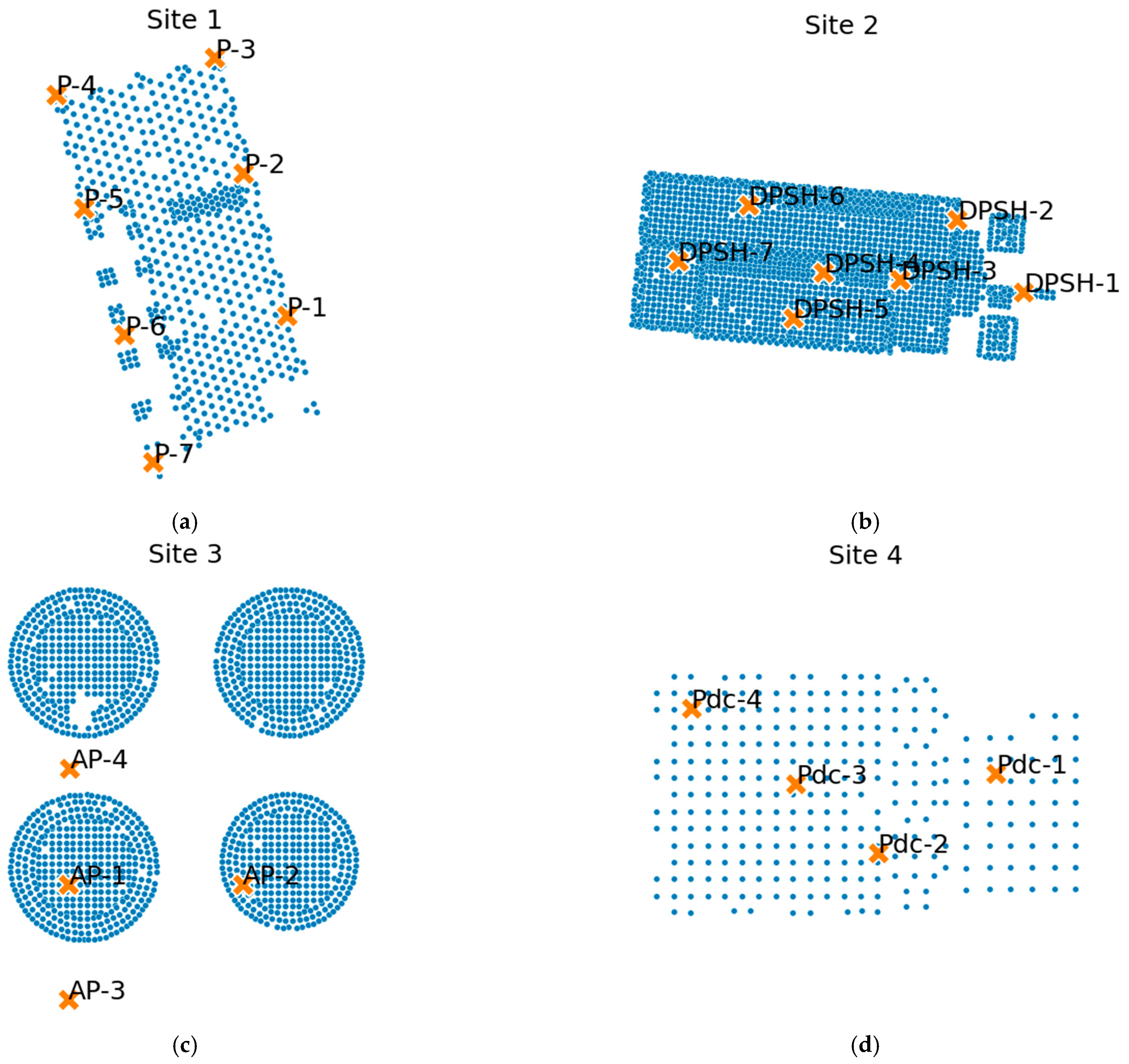
In this study, a significant amount of data obtained from the MWD system from deep foundation and ground improvement machinery is analyzed. Figure 1 shows the plan views of the four sites studied. The circles represent the perforations made; the crosses are the penetrometers available. The aim was to correlate said penetration tests with the values obtained from MWD using ML techniques, specifically decision trees and random forests.

The significance of this research lies in the fact that, at the time of writing, it is the first time that this approach has been applied to rigid inclusions execution data.

The input variables have been the drilling speed (m/h), rotation speed (rpm), rotation torque (t·m) and thrust (t). The objective variable has been the blow values of dynamic penetrometers.

The results obtained show that the algorithms have been able to relate, with a certain degree of precision, the drilling parameters with the blows of the penetrometers. This information allows an increase in the level of security, an adaption of the execution to the real conditions of the ground and detection of possible anomalies, among other things.

The structure of the paper is the following:

• The related works are described.
• MWD in pile driving and soil improvement machinery is presented.
• The decision trees and random forests algorithms are summarized.
• The methodology followed is explained.
• The analyzed sites are described.
• The results obtained are shown and discussed.
• The conclusions are drawn.

2. Related Works

Geotechnical engineering hosts problems with many uncertainties in which the true relationships among the variables are unknown. This makes it an interesting field for the application of ML algorithms. In this way, several authors have used this approach [10], especially through the application of neural networks (NN).

In the field of layer characterization, Shuku et al. [13] proposed a new method for estimating trends and layer boundaries in depth-dependent soil data based on lasso. This new method (SBLasso) was applied to synthetic data, as well as an actual CPT sounding taken at Texas A&M University and it provided stratification consistent with existing methods.

Zhao and Wang [14] proposed an interpolation first method to characterize a multilayer soil property profile when measurements within each layer are sparse and limited. This method interpolates the multilayer soil property profile using measurements from all layers together as input to a Bayesian supervised machine learning first. Then, the interpolated multilayer soil property profile is stratified using an unsupervised machine learning method, e.g., the modified k-means clustering method.

Focusing on the use of MWD, Rai et al. [15] reviewed MWD techniques in the extractive industry, and therefore focused on rock drilling. Kadkhodaie-Ilkhchi et al. [16] conducted a comparative study of three machine learning techniques using MWD data from drilling for explosives at an iron mine in Australia. Other studies related to the recognition of rocks using MWD and ML have also been published with such references [17,18,19,20].

In the field of soils and civil engineering, Goh [21,22] estimated the load-bearing capacity of driven piles using NN in non-cohesive soils from data collected by Flaate [23] for wooden, precast concrete and steel piles. The input parameters were hammer weight, hammer drop height, hammer type, pile length, pile weight, pile modulus of elasticity, pile cross-sectional area, and pile set. The target value was the load-bearing capacity of the pile. The model was able to obtain high correlation coefficients between the input parameters and the load-bearing capacity for both the train set and the test set. Furthermore, NN were found to perform better than classical formulas when predicting load-bearing capacity.

Lee and Lee [24] also used NN to calculate the load-bearing capacity of piles. Five input variables were used: penetration depth ratio, the average SPT strike along the axis of the pile, the average SPT strike near the tip of the pile, the penetration rate for each strike and the hammer energy. The results obtained were compared with the Meyerhof formula [25]. The values obtained through NN correlated better with the measured values than those obtained through the Meyerhof equation.

Although the input parameters did not come from MWD, Teh et al. [26], proposed an NN model to estimate the load-bearing capacity of piles from dynamic pressure wave data. The data came from 37 precast piles from 21 different sites. The objective parameters were the values of the soil parameters predicted by the CAPWAP model [27]. This approach to predicting parameter values is similar to what is considered in this article.

In another use of NN, Diaz et al. [28] predicted the rate of penetration during wellbore drilling using data obtained as the drilling progresses within a given well.

Pal and Deswal [29] used a Gaussian regression process (GP) to predict the load-bearing capacity of the pile. Part of the input data was the same as that used by Goh. The performance of the proposed model was compared with support vector machines (SVM) and empirical relationships, obtaining a better result.

Galende-Hernández et al. [30] carried out a study estimating the value of the RMR from the characterization of the excavation face of a tunnel, using MWD and expert knowledge in the execution of a tunnel using explosives. The results obtained showed a good correlation. Such work posed a similar philosophy to that of this article since it sought to estimate the value of a soil parameter (the RMR) from the drilling parameters.

Although several examples of the use of MWD and ML data have been collected, the use of data obtained directly from machinery is relatively scarce. In this proposal, data from construction sites was taken directly from the MWD system and used to estimate the values of the dynamic penetrometer. The objective was to reach results for each perforation to be equivalent to having carried out a penetration test. Although data from rigid inclusions with ground displacement has been used, the methodology is general enough to be applicable to other works.

3. MWD in Pile Driving and Soil Improvement Machinery

The current pile machinery has a series of measuring instruments that allow the collection of performance data. The main information obtained during rotary drilling usually consists of the following [31]: the length of the drilling, drilling speed (V_A), rotation speed (V_R) and the hydraulic pressures of the rotary and thrust motors. These data are obtained with a high frequency, for example, every 10 cm of perforation.

3.1. Direct and Indirect Parameters

The parameters obtained from MWD can be divided into two groups depending on the process of attainment: direct parameters and indirect parameters.

Directly obtained parameters are those in which it is not necessary to apply any type of correlation to the values obtained from the sensors. Depth, rotational speed, and drilling speed can be considered direct parameters as they are obtained directly or as a function of time. Perhaps the most relevant of this type of parameter is the drilling speed as it is very indicative of the hardness of the terrain.

However, other parameters such as thrust force (P_O) and rotation torque (C_R) are obtained through mechanical correlations from the hydraulic pressure of the motors. These values (although they can be provided by the manufacturer) depend on a multitude of factors: the efficiency of the motor, the configuration of the machinery at any given time, the wear of the components, and so forth. Consequently, it is exceedingly difficult to know the true value of these parameters. These possible sources of error must be considered when analyzing the results obtained when using parameters that do not come from direct measurements. To this type of error attributed to the correlations, the errors and tolerances of the measuring devices must also be added.

3.2. Compound Indices and Parameters

Drilling parameters are related to soil resistance. However, by taking these parameters separately, the relationship is not clear. For this reason, various authors have developed compound parameters that combine individual parameters into energy expressions or empirical indices seeking to show the strength of the ground from the drilling data.

Most of these parameters or compound indices follow the same basic structure. In this way, the hardness of the ground is directly proportional to the rotation torque and the applied load and inversely proportional to the area of the drilling and drilling speed. These relationships tend to soften the profile, giving them greater physical meaning and making their interpretation easier. The most common of these indices are listed in

Table 1. Most used compound parameters.

Name	Formula	Units	Ref.
Penetration resistance	$R_p={\left(t\right)}_{dZ=0.2m}$	s/0.2 m	Möller et al., 2004 [33]
Somerton index	$S_d\approx P_E{\left(\frac{V_R}{V_A}\right)}^{\frac{1}{2}}\approx \frac{P_O}{\sqrt{V_A}}$	kPa	Somerton 1959 [34]
Drilling specific energy	$SDE=\frac{P_O}{S_0}+\frac{2\pi }{S_0}·\frac{V_{R}x{C}_R}{V_A}$	kJ/m3	Teale 1965 [35]
Specific energy	$E_S=C_R·\frac{V_R}{V_A}$	N·m/m	Pfister 1985 [36]
Normalized energy	$E_N=\frac{\alpha P_o{V}_A+\beta C_{R}2\pi V_R+\gamma P_{M}f}{V_A}$	N·m/m	Nishi et al., 1998 [37]
Alteration index	$I_a=1+k_0\left(\frac{P_O}{P_{max}}-k_1\frac{V_A}{V_{max}}\right)$	-	Pfister 1985 [36]
Entropy of S	$L\left(z\right)={\displaystyle {\displaystyle \sum }_{Z_0}^Z}\left|S\left(z+dz\right)-S\left(z\right)\right|$	-	Duchamp 1988 [38]

[32].

Of these parameters, penetration resistance, Somerton’s index, and drilling specific energy are intended for research in hard rock and soils or for recording parameters during on-site testing. Their application to soft soils, based on MWD data, can be difficult to interpret.

The main obstacle with these formulas is that they assume a form of the relationship between the parameters and the strength that, although logical, does not necessarily correspond to reality. Therefore, these formulas give us a qualitative idea of the resistance to perforation and are useful when the differences in behavior within the soil are clear, but they do not supply precise figures.

4. Decision Trees and Random Forests

4.1. Decision Trees

Decision trees (DT) are a popular algorithm for classification or regression capable of providing reliable and easily interpretable results.

Although there are a variety of DT algorithms, they all have a similar structure. To be concise, the algorithm consists of dividing the data set into successive subsets following established rules. This process can be represented graphically in structures that resemble a tree (Figure 2).

The success of DTs is explained by several factors that make them quite useful in practice [39]:

• DTs are non-parametric. They do not assume the way in which the variables are related, and they are able to model complex interactions.
• They handle heterogeneous data (numbers, categories, or a mix of both).
• In their own operation, DTs implement the choice of the most important variables, making them robust (up to a point) against irrelevant variables.
• They are equally robust against outliers and sorting errors.
• They are easy to interpret, even for users without previous knowledge of statistics.

Building a decision tree consists of three parts: division rules, stop criteria and assignment rules.

4.2. Division Rules

A division at a node can be understood as a question whose answer divides the set at the node into two or more subsets. These questions or division rules vary depending on the type of decision tree chosen. Once these rules have been applied to each of the variables in the set, they are ordered according to the information they provide, establishing the most useful division as a node.

The application of these criteria defines the shape of the tree.

4.3. Stop Criteria

Overfitting refers to the situation where the model fits the training data too much, leading to larger errors in the test data. To avoid this problem stopping criteria can be set. This set of rules can be regulated to achieve trees that are neither too short (too general) nor too long (overfitting problem).

The tree will stop its development by itself in two cases:

• When the objective values are homogeneous in all samples of the node.
• When the input values are constant in the node.

In the previous cases, it is not possible to gain purity in the nodes by continuing the divisions, so the algorithm stops. These nodes that are not divided are called leaf nodes. In addition to these situations, other criteria can be added. The most common approaches are:

• Set a node as a leaf node if it contains less than a minimum number of samples.
• Set a maximum node depth. In this way, the number of divisions that the algorithm performs is limited.
• Establish a node as a leaf node when the impurity decrease is less than a certain threshold.
• Establish a node as a leaf node if it is not possible to establish dependent nodes with a minimum number of samples.

All these criteria must be defined by the user looking for the most adequate balance. Such balance can be difficult to achieve, which is why specially dedicated models are commonly used at the expense of a greater computational load.

These stopping criteria can be understood as a method of pruning the tree. Specifically, they are pre-pruning methods that are carried out during the growth of the tree.

Another method would be to develop the entire tree and perform the pruning eliminating those nodes that provide the worst results in a different data set than that used to generate the tree. This method usually provides better results than pre-pruning.

4.4. Assignment Rules

The assignment rules refer to the criteria followed to assign a value to a leaf node. In this way, in regression problems, it would be assigned to the value that provides the smallest mean square error. In a classification problem, the value would be that of the most probable category.

4.5. Implementation of DT in Scikit-Learn

For the application of DT and RF, the Scikit-learn library has been used. Scikit-learn [40] is a Python module that integrates a wide range of machine learning algorithms. It is a package designed for non-experts, focused on the ease of use, documentation, and consistency of the application programming interface (API).

The learning is carried out using the fit method together with the train values (in the case of supervised learning, these values would be X_train and y_train tables for input variables and target variables to predict, respectively). During the definition of the model, the hyperparameters that control the algorithm are introduced. The following pseudocode shows an example of DT training where the minimum number of samples to divide the node is five.

        # Import the required module
        from sklearn.tree import DecisionTreeClassifier,
        # Definition of the model and hyper-parameters
        clf = DecisionTreeClassifier(min_samples_split=5),
        # Learning the model from the data
        clf.fit(X_train, y_train),
		

The predictions are made with the prediction interface once the algorithm is trained, as shown in the next pseudocode.

        # Make predictions from new data.
        y_pred = clf.predict(X_test),
		

In addition, the prediction interface implements methods to check the confidence level of the prediction, as well as a score function to evaluate the performance of the model.

Lastly, the transformation interface allows the making of changes to the data, such as adjusting it to a normal distribution, which may be necessary when executing some algorithms.

As already mentioned, the selection of the best hyperparameters of a model can be a complex task. For this, scikit-learn implements two meta-estimators, GridSearchCV and RandomizedSearchCV. Both take as data an algorithm, those hyperparameters that must be used and a series of values to search through. GridSearchCV performs all possible combinations, while RandomizedSearchCV performs a fixed number of iterations. These meta-estimators perform a cross-validation method (CV). To do this, the data set is divided again into a train set and a test set. For each combination of hyperparameters and each generated train/test pair, GridSearchCV and RandomizedSearchCV adjust their estimator on the train set and evaluate their performance on the test set. In the end, the best-performing model is retained as the best set of hyper-parameters.

Within the multiple decision tree algorithms, scikit-learn implements an optimized version of Classification and Regression Trees (CART [41]), although it does not yet support non-numeric input variables.

4.6. Hyper-Parameters of Decision Trees in Scikit-Learn

Table 2. Hyper-parameters for classification decision trees in scikit-learn 0.21.

Parameter	Default Value	Description
criterion	‘gini’	Function to assess the quality of the division. The criteria supported are ‘gini’ for Gini impurity and ‘entropy’ for information gain.
splitter	‘best’	Strategy used for choosing the division. The supported strategies are ‘best’ and ‘random’.
max_depth	None	Maximum depth of the tree. If the value is ‘None’, the nodes will continue until all are pure or until all leaves contain less than min_samples_split samples.
min_samples_split	2	Minimum number of samples required to divide a node.
min_samples_leaf	1	Minimum number of samples required in a leaf node. A node will only be split if the result has at least min_samples_leaf samples.
min_weight_fraction_leaf	0.0	Minimum weight of a leaf node. Samples have equal weight when sample_weight is not provided.
max_features	None	The number of characteristics to consider when looking for the best division.
random_state	None	Parameter that controls the randomness of the model.
max_leaf_nodes	None	Maximum number of leaf nodes.
min_impurity_decrease	0.0	A node will divide if that division induces a decrease in impurity greater than or equal to this value.
min_impurity_split	0	A node will split if its impurity is above this value.
class_weight	None	Weights associated with the classes. If no value is provided, all classes will be assumed to have a weight of one.

shows the hyper-parameters of the implementation in scikit-learn of the classification decision trees.

4.7. Implementation of RF in Scikit-Learn

Unlike the original publication [42], the scikit-learn implementation combines classifiers by averaging their probabilistic prediction, instead of letting each classifier vote for a single class.

When building an RF in scikit-learn you can control the same parameters as for a DT in addition to specific RF hyperparameters. That is, the characteristics of the individual trees that make up the forest can be controlled. However, the main objective of the calibration of these parameters is to avoid overfitting the tree, which is partly avoided by the very way of constructing the RF. In this way, we can allow fully developed trees to form, at the cost of a higher computational cost. There are therefore two parameters to adjust: n_estimators and max_features.

n_estimators is the number of trees in the forest. In principle, the more the merrier. However, from a certain number of trees, there is no improvement in the prediction, and it must be considered that each tree increases the calculation time.

max_features is the size of the random subsets of features to consider when splitting a node. The lower this value, the greater the reduction in variance, but also the greater the increase in bias. In practice, as stated in the scikit-learn documentation, values of max_features = None (always considering all characteristics instead of a random subset) work well for regression problems, and max_features = “sqrt” (using a subset random size sqrt (n_features)) for classification tasks (where n_features is the number of features in the data).

Since we are treating the problem as classification, we will use max_features = “sqrt”.

To define the optimal number of trees, an iterative calculation can be carried out to check the increase in the quality of the prediction. In this way, it can be verified at which point the increase in the number of trees no longer compensates.

5. Methodology

The main objective of this study was to predict the values of the dynamic penetrometer based on the drilling parameters. This test was chosen because it is abundant and easy to interpret, which makes the results obtained more useful. In fact, these tests are frequently used for the design of deep foundations and soil treatments.

The first step was to collect the data analyzed in an easy-to-use format from the four sites. This translated into transforming the data from the MWD files into a depth-based table format and adding necessary data such as the positions of each column.

Once the data had been adapted, it was necessary to assign a blow value to each row of data according to the closest penetrometer. In this sense, it was essential to pay attention to the execution levels of both the penetrometers and the columns.

The data were treated by eliminating anomalous values based on knowledge of the characteristics of the soil and the machinery used. The resulting values were divided into a train set and a test set, using the first set to train the decision tree and random forests algorithms. Once trained, the performance of the algorithms was checked with the test set (Figure 3).

6. Summary of the Analyzed Sites

Four different sites have been studied (Figure 1) in which the soil improvement method controlled modulus columns have been used [43]. The execution procedure has been by means of a displacement helix. This method moves the drilled soil to the sides without extracting it.

It must be considered that this drilling method presents a different behavior than a cutting tool, mobilizing the lateral resistance of the ground traversed.

These columns were executed using a drilling rig similar to an Enteco E6050.

6.1. Site 1

This site consisted of treating the ground under the slab and footings of an industrial building, making a total of 665 rigid inclusions of 300 and 360 mm in diameter.

During the geotechnical campaign, a total of 7 Dynamic Probing Super Heavy (DPSH) penetrometers were carried out, among other works.

The surface layer of the soil is formed by an anthropic fill of poured silty sands with an interpreted thickness that varies between 1.60 and 2.20 m. Under these fillings, a layer of vegetal soil of little thickness appears (between 0.4 and 1.0 m), also composed of silty sands. This is followed by an alluvial level of fine sand with silt of very loose compacity and a thickness of 1.60 to 2.20 m. The last layer investigated consists of the altered granite of the area with increasing compactness in depth.

The material is, therefore, of a homogeneous nature and mainly sandy, due to the water table being close to the surface. Figure 4 shows the DPSH tests carried out on site 1. The points represent the number of blows required to advance 20 cm depending on the depth.

6.2. Site 2

Site 2 also consisted of treating the ground under an industrial warehouse using 360 mm diameter inclusions.

In this case, a total of 7 DPSH penetrometers are available.

According to the geotechnical information, the first level is formed by anthropic fillings with an average thickness of 6 m made up of sands and clayey sands (SC). Below this level, alluvial materials appear arranged in layers of diverse nature, forming an interlayer from clays to sands, although with some lateral continuity. This level can reach a depth of about 30 m. The last level detected coincides with the Pliocene substrate in the area, made up of dense, highly compact sands. This level is at such a depth that it is not reached by the soil treatment.

The water table has been detected at very different levels depending on the time of the measurements. It has varied between 2 and 8 m deep.

Therefore, unlike site 1, this site presents a much more heterogeneous geology, with materials of different nature and a variable position of the water table. Figure 5 shows the DPSH tests carried out on site 2.

6.3. Site 3

Site 3 consisted of soil treatment using 360 mm diameter controlled modulus columns for the construction of hydrocarbon tanks on a port landfill.

In this work, the information on four penetrometers is available. However, these were made before knowing the final position of the tanks, which finally did not coincide with that of all penetrometers. Due to this circumstance, only two of them are relevant (see lower left of Figure 1).

The port landfill consisted of material from dredging used to fill various areas reclaimed from the sea. The composition is variable but mainly granular, formed by sands with traces of fines and gravel. The thickness of this fill is between four and eight meters. Below this first level is the natural terrain composed of quaternary sands that increase in compactness with depth.

The water table is very superficial and will depend mainly on the level of the sea.

In this case, the terrain is again mainly sandy and reasonably homogeneous.

DPSH tests for site 3 are shown in Figure 6.

6.4. Site 4

This works consisted of treating the ground under an industrial warehouse and exterior pavements with inclusions of 300 and 360 mm in diameter.

The number of penetrometers available for this work was four.

In this case, the soil is made up of an anthropic fill of sand and silt of low plasticity with a thickness of about 7 m. Below this level, there is a terrace deposit formed by silts and sandy clays and silty sands of reddish colors, fine grain and low plasticity.

The water table is about 6 m deep on average.

Unlike the previous cases, the penetrometric tests carried out in this site were Borro type instead of DPSH.

In the case of site 4, the Borro test values are shown in Figure 7.

6.5. Available Data

The parameters were recorded with Menard’s Emparex data acquisition system which provides data approximately every 8 cm of drilling. Said values, ignoring those of general information about the site, are shown in

Table 3. MWD available data.

Parameter	Name of the Column	Depth from Start of Drilling	Drilling Speed	Rotation Speed	Rotary Torque Pressure	Crowd Pressure	Torque	Crowd
Unit	-	m	m/h	rpm	bar	bar	t·m	t

.

It should be noted that torque and crowd parameters are calculated from rotary torque pressure and crowd pressure, respectively.

In order to narrow down the analysis carried out, a single diameter has been considered for each work (360 mm in sites 1, 2 and 3 and 300 mm in site 4, according to the most common diameter in each site) and the nature of the terrain has not been taken into account as a variable (this is mainly granular in the sites analyzed). However, in the future, it will be necessary to add at least both parameters to the analysis. In this way, the number of initially available data is shown in

Table 4. Data initially available.

Site	Columns	Data Rows
Site 1	159	20,916
Site 2	2096	269,921
Site 3	1504	111,428
Site 4	287	27,797

.

The input variables for the algorithms are drilling speed, rotation speed, torque, and crowd. These variables are the same used for the compound parameters of Table 1. The target variable is the number of blows to advance 20 cm of the penetrometers.

6.6. Initial Treatment of the Data

It has been verified that there is no missing data. That data without associated penetrometer value (in the case of the closest penetrometer being short or has started at a lower level than the level of execution of the inclusions) has been deleted. In the type of problem of this research, missing data should not be an issue. Nevertheless, for an in-depth discussion about that topic, the work of Duy-Tai Dinh et al. [44] can be studied.

The penetrometer data is highly affected by specific high values that do not reflect the real resistance of the ground and are therefore not translated into the resistance to perforation. In order to attenuate this effect, the stroke values at each point have been transformed to the mean of the point itself and the values above and below it. Stroke values greater than 30 have also been removed.

It has also been verified that the values obtained in the registry are in line with what is expected depending on the machinery used. In this type of machine, the relationship between the torque pressure and the applied torque depends on the rotational speed of the tool. Figure 8 represents the measured torque pressure and the rotation torque calculated by the parameter recording system for the case of site 1. The result is several lines with different slopes depending on the rotation speed. Abnormal values associated with low rotational speeds are observed, such as negative or very high torque values. It is also verified in the graph on the right that these values are associated with shallow depths. That is, these values are associated with the beginning of drilling and are not representative.

In this way, these values, which do not correspond to the expected normal behavior, are not considered when carrying out the study. The corrected graph is shown in Figure 9.

7. Results

The algorithms have been trained to predict the blow values of the DPSH penetrometer. These values are discrete in nature and the problem can be treated as both a regression or a classification. In this case, it was decided to use the classification algorithms with 31 classes (from 0 to 30 blow values). However, since the target variable values are numbers, regression metrics can also be used.

To evaluate the performance of the predictions, the accuracy (Equation (1)), Pearson’s correlation coefficient (Equation (2)), MAE, MSE and R² were used.

$$accuracy \left(y,\widehat{y}\right)=\frac{1}{n_{samples}}{{\displaystyle \sum }}_{i=0}^{n_{samples}-1}I\left({\widehat{y}}_i=y_i\right)$$

(1)

$${\rho }_{X,Y}=\frac{{\sigma }_{XY}}{{\sigma }_X·{\sigma }_Y}$$

(2)

$$MAE=\frac{{{\displaystyle \sum }}_{i=1}^n\left|y_i-{\widehat{y}}_i\right|}{n}$$

(3)

$$MSE=\frac{{{\displaystyle \sum }}_{i=1}^n{\left(y_i-{\widehat{y}}_i\right)}^2}{n}$$

(4)

$$R^2\left(y,\widehat{y}\right)=1-\frac{{{\displaystyle \sum }}_{i=1}^n{\left(y_i-{\widehat{y}}_i\right)}^2}{{{\displaystyle \sum }}_{i=1}^n{\left(y_i-\overline{y}\right)}^2}$$

(5)

Accuracy measures the proportion of correctly classified samples out of the total. In this case, the Pearson correlation coefficient measures the linear relationship between the real values of the target variable and the values calculated by the algorithms.

In the various sites analyzed, the models have been trained for a single diameter of those available since it is not the objective of this article to evaluate the effect of the different diameters.

In addition, only those perforations made less than 2 m from its associated penetrometer have been considered. In this way, an attempt is made to avoid errors due to changes in the terrain with the distance to the penetrometer. The effect of separation is evaluated later in this article. This limitation greatly affects the number of samples available (

Table 5. Data at a distance ≤2 m from its associated penetrometer.

Site	Columns	Data Rows
1	10	1375
2	12	1030
3	6	536
4	6	549

).

The input variables are the drilling speed (m/h), rotation speed (rpm), rotation torque (t·m) and thrust (t). Therefore, the same parameters as in traditional formulas are considered. The variable to predict is the blow values per 20 cm of the penetrometers.

For every calculation, the data set is divided randomly into a train set with 70% of the data and a validation set with the remaining 30%.

7.1. Fully Developed Trees

As a first approximation, fully developed DTs are used, without restrictions on their growth. This is achieved with the default Scikit-learn parameters.

Table 6. Correlations obtained for a fully developed DT.

Site	Set	Accuracy	Correlation Coefficient	MAE	MSE	R2
1	Test	0.15 (±0.02)	0.62 (±0.04)	4.10 (±0.20)	35.03 (±3.36)	0.28 (±0.08)
	Train	1.00 (±0.00)	1.00 (±0.00)	0.00 (±0.00)	0.00 (±0.00)	1.00 (±0.00)
2	Test	0.27 (±0.03)	0.42 (±0.07)	2.59 (±0.17)	17.06 (±2.38)	−0.20 (±0.16)
	Train	1.00 (±0.00)	1.00 (±0.00)	0.00 (±0.00)	0.00 (±0.00)	1.00 (±0.00)
3	Test	0.32 (±0.03)	0.57 (±0.09)	3.00 (±0.30)	22.48 (±3.70)	−0.09 (±0.20)
	Train	1.00 (±0.00)	1.00 (±0.00)	0.00 (±0.00)	0.01 (±0.00)	1.00 (±0.00)
4	Test	0.15 (±0.02)	0.24 (±0.08)	5.34 (±0.38)	59.72 (±7.55)	−0.38 (±0.20)
	Train	1.00 (±0.00)	1.00 (±0.00)	0.00 (±0.00)	0.00 (±0.00)	1.00 (±0.00)

shows accuracy, correlation coefficient, MAE, MSE and R² values for a fully developed DT. These values vary slightly when you rerun the algorithm due to random effects even for the same train-test split. The algorithm has been tested on 500 different train-test splits. The mean values are shown in the tables with their standard deviation in brackets.

The models overfit since a perfect correlation is achieved for the train set while the correlation is much lower in the test set. In addition, fully developing the trees has resulted in trees between 150 and 650 leaves, which makes their interpretation impossible. Furthermore, the R² values for the test set are very low. Although their deviation is also very high, such low values of R² seem to be caused by the outliers.

7.2. Hyperparameter Calibration Using GridSearchCV

In order to find the best hyperparameters, the GridSearchCV meta-estimator has been used. Although it would be possible to calibrate all hyperparameters, due to the nature of the data analyzed, not all of them are relevant.

Table 7. Hyperparameters used during calibration with GridSearchCV.

Hyperparameters	Criterion	Splitter	Max_depth	Min_samples_split	Min_samples_leaf	Max_leaf_nodes
Values	Gini, entropy	Best, random	1, 5, 10, 15, None	2, 4, 6, 8	1, 2, 3, 4, 5	None, 400, 200, 100, 50, 10

shows the set of hyperparameters introduced in GridSearchCV.

To perform this calculation, a random_state = 42 has been established. This way, GridSearchCV always works on the same data set, obtaining very similar results regardless of how many times the calculation is made (

Table 8. Best parameters obtained by GridSearchCV.

Site	1	2	3	4
criterion	gini	gini	gini	gini
splitter	random	random	random	random
max_depth	None	15	10	10
min_samples_split	2	8	2	4
min_samples_leaf	1	1	1	1
max_leaf_nodes	400	400	50	100

). However, it must be considered that different sets can give rise to different hyperparameters that may be better or worse than those obtained in this case.

With the new calculated hyperparameters, there is less overfitting than for fully developed DTs. However, the predictability of the validation set is not significantly improved (

Table 9. Correlations obtained using GridSearchCV.

Site	Set	Accuracy	Correlation Coefficient	MAE	MSE	R2
1	Test	0.12 (±0.02)	0.62 (±0.04)	4.08 (±0.26)	34.56 (±4.34)	0.29 (±0.09)
	Train	0.64 (±0.22)	0.88 (±0.08)	2.46 (±0.92)	21.24 (±7.96)	0.56 (±0.16)
2	Test	0.23 (±0.03)	0.49(±0.07)	2.52(±0.18)	15.99 (±2.34)	−0.12(±0.14)
	Train	0.53 (±0.21)	0.60 (±0.15)	1.40 (±0.55)	9.33 (±3.77)	0.35 (±0.26)
3	Test	0.32 (±0.02)	0.34 (±0.10)	2.99 (±0.29)	24.92 (±4.13)	−0.20 (±0.14)
	Train	0.60 (±0.08)	0.54 (±0.11)	2.63 (±0.35)	22.19 (±3.71)	−0.07 (±0.17)
4	Test	0.14 (±0.02)	0.24 (±0.11)	5.27 (±0.44)	61.56 (±9.19)	−0.41 (±0.17)
	Train	0.50 (±0.16)	0.54 (±0.18)	3.92 (±0.94)	47.35 (±12.41)	−0.09(±0.28)

). On the other hand, there is a reduction in the complexity of the model (fewer leaf nodes and less depth). This would make the use of hyperparameters calculated using GridSearchCV preferable (

Table 10. Complexity of fully developed trees compared to those obtained through GridSearchCV.

	Fully Developed Tree		GridSearchCV
Site	Depth	Leaf Nodes	Depth	Leaf Nodes
1	20	681	20	400
2	22	437	15	177
3	16	180	10	50
4	20	269	10	100

).

7.3. Random Forests

Figure 10 shows the evolution of the accuracy as a function of the number of trees considered for site 1. It has been verified that with a number of trees in the order of 50, it is ensured that the maximum precision has been reached. The calculation has been performed with 75 trees.

Table 11. Correlations obtained for RFs.

Site	Set	Accuracy	Correlation Coefficient	MAE	MSE	R2
1	Test	0.18 (±0.02)	0.76 (±0.02)	3.45 (±0.02)	26.81 (±0.02)	0.45 (±0.02)
	Train	1.00 (±0.00)	1.00 (±0.00)	0.00 (±0.00)	0.00 (±0.00)	1.00 (±0.00)
2	Test	0.31 (±0.03)	0.54 (±0.06)	2.15(±0.13)	12.82(±1.84)	0.10(±0.11)
	Train	1.00 (±0.00)	1.00 (±0.00)	0.00 (±0.00)	0.00 (±0.00)	1.00 (±0.00)
3	Test	0.38 (±0.03)	0.57 (±0.07)	2.60 (±0.24)	20.03 (±3.05)	0.04(±0.13)
	Train	1.00 (±0.00)	1.00 (±0.00)	0.00 (±0.00)	0.01 (±0.00)	1.00 (±0.00)
4	Test	0.18 (±0.02)	0.28(±0.07)	4.83 (±0.36)	54.30 (±7.00)	−0.26(±0.16)
	Train	1.00 (±0.00)	1.00 (±0.00)	0.00 (±0.00)	0.02 (±0.00)	1.00 (±0.00)

shows the values of the metrics for RFs.

The results obtained with RF are better than those obtained in all the analyzed metrics.

7.4. Comparison with Compound Parameters

Table 12. Correlation coefficient for the compound parameters.

Compound Parameter	Site
	1	2	3	4
Penetration resistance	−0.45	−0.09	−0.40	−0.24
Somerton index	0.40	−0.07	0.42	0.12
Drilling specific energy	0.52	0.13	0.44	0.34
Specific energy	0.44	0.02	0.48	0.32
Alteration index	0.49	0.14	0.39	0.29
DT	0.62	0.42	0.57	0.24
DT (GridSearch CV)	0.62	0.49	0.34	0.24
RF	0.76	0.54	0.57	0.28
Linear regression	0.56	0.39	0.49	0.36

shows the values of the correlation coefficient between the blows of the penetrometers and the results of both the analytical formulas and the algorithms used. The values obtained by linear regression are also shown, in order to compare with the simplest possible ML algorithm.

As can be seen, the ML algorithms show a higher correlation with the penetrometers than the compound parameters in all sites except for site 4, where similar values of the correlation coefficient are obtained. DT and RF outperform linear regression in three of the four sites.

7.5. Representation of Data as a Function of Depth

Unlike other machine learning problems, in our case it is possible to represent the data with ease, showing the blow values obtained versus depth.

Figure 11, Figure 12, Figure 13 and Figure 14 show real and calculated values versus depth for the test subset. The first graph of each figure corresponds to the real blow values per 20 cm, the second are the values obtained from a fully developed DT and the third is the values for RF. These images quickly show the ability of the algorithms to reproduce the penetrometric profile of the soil.

7.6. Advantage of Taking Depth into Account

The variables used in the previous sections (drilling speed, rotational speed, torque and thrust force) have been the same as those considered in the classical formulas.

However, when proposing a machine learning algorithm, it may be interesting to also use depth. In this way, the algorithm should be able to detect different layers on the ground and give values more in line with reality. As can be seen in

Table 13. Correlations obtained for fully developed DTs with depth.

Site	Set	Accuracy	Correlation Coefficient	MAE	MSE	R2
1	Test	0.42 (±0.03)	0.87 (±0.18)	1.97 (±0.15)	11.98 (±1.74)	0.76 (±0.04)
2	Test	0.30 (±0.03)	0.61 (±0.07)	1.70 (±0.16)	9.81(±2.12)	0.31(±0.15)
3	Test	0.64 (±0.73)	0.94 (±0.24)	0.65 (±0.15)	2.32 (±1.01)	0.89 (±0.05)
4	Test	0.35 (±0.04)	0.62 (±0.07)	3.10 (±0.33)	29.06 (±5.80)	0.32 (±0.15)

and

Table 14. Correlations obtained for RFs with depth.

Site	Set	Accuracy	Correlation Coefficient	MAE	MSE	R2
1	Test	0.38 (±0.03)	0.90 (±0.01)	1.66 (±0.11)	8.82 (±1.21)	0.82 (±0.03)
2	Test	0.38 (±0.04)	0.74 (±0.05)	1.35 (±0.12)	6.54 (±1.56)	0.54 (±0.09)
3	Test	0.50 (±0.06)	0.91 (±0.03)	0.90 (±0.13)	3.74 (±1.17)	0.82 (±0.05)
4	Test	0.33 (±0.03)	0.62 (±0.50)	2.70 (±0.27)	22.68 (±4.72)	0.48 (±0.10)

, the increase in prediction precision is very important. Figure 15, Figure 16, Figure 17 and Figure 18, show that the profile obtained with the models, considering the depth, is practically identical to the real one.

7.7. Increase in Error with Distance to Perforations

Normally, only a few penetrometers are carried out and, subsequently, there will not be too many columns near such tests. This greatly limits the relevant data, resulting in a handicap when using certain algorithms.

The calculations performed up to this point have only considered data that was within 2 m or less of its associated penetrometer.

Through an iterative calculation, the increase in error has been verified, based on the F-score and the correlation coefficient as the distance to the perforation increases. It must be borne in mind that this error depends on the type of soil. With a homogeneous layer distribution (with horizontal continuity) in the soil, the error should not be large, but it can be important in highly variable terrain.

The results obtained for the different sites (for fully developed DTs and taking depth into account) are shown in Figure 19.

As can be seen, the precision is maximum when distances between columns and the penetrometer are small (in the order of 2 m). From that point, there is a rapid decline in the first few meters which later slows down.

In sites 3 and 4, the point of maximum precision does not occur with the minimum distance but instead, a little further. This may be due to the bias that would occur when considering very small samples.

According to the values obtained and considering the high degree of uncertainty commonly associated with geotechnical works, the increase in error with distances to penetrometers greater than 2 m can be considered acceptable when making predictions if there are not enough values in closer distances.

7.8. Application to a Set of Sites

As a culmination of the analysis carried out, the operation of the algorithm has been verified with a set of sites. Many are the factors that can vary from one job to another in terms of soil behavior, equipment performance and so on.

The same calculations shown in the previous sections have been carried out for sites 1, 2 and 3. Site 4 has been omitted since the penetrometers executed were Borro type instead of DPSH, as in the rest of the sites.

When applying the algorithms to the data set of the three sites, the results are equally promising, as reflected in

Table 15. Correlations obtained for the set of sites 1, 2 and 3.

Site	Model	Set	Accuracy	Correlation Coefficient	MAE	MSE	R2
1, 2, 3	Fully developed DT with depth	Test	0.35 (±0.03)	0.82 (±0.02)	1.92 (±0.10)	11.84 (±0.18)	0.69 (±0.03)
	RF with depth	Test	0.37 (±0.02)	0.88 (±0.01)	1.52 (±0.07)	7.77 (±0.83)	0.80 (±0.02)

and Figure 20.

The precision obtained is similar to the average of the three sites separately. It therefore seems possible to analyze all the sites without producing a significant increase in error. It should be noted, however, that the materials of the works studied are of a similar nature. It will be necessary to evaluate in the future the effect of materials of a different composition.

8. Discussion and Conclusions

In this article, the application of machine learning algorithms to correlate data obtained from MWD with dynamic penetrometer values has been studied.

Decision tree algorithms and random forests have been used to predict penetrometer values, unlike in other studies where neural networks have been used. These algorithms have a simpler implementation as few parameters must be adjusted and these are easy to interpret. The graphical representation of the results is even possible, although in this case, it has not been practical due to the large number of resulting nodes. This simplicity, together with the existence of libraries such as scikit-learn [45], allow an easier application.

The study has been carried out from real execution data. It is not common to have data from sites, as most of the previous studies use laboratory data or historical cases from the bibliography. In addition, many of the existing cases with MWD data are from rock drilling and not soils, as in this article.

The results obtained have shown that, for the four sites studied, a fully developed decision tree is capable of achieving great precision. The importance of taking depth into account in the calculations has also been shown since it significantly increases the degree of correlation. It should be noted, however, that the number of penetrometer tests available is low and giving excessive importance to depth could mask terrain of a difference in nature if the soil profile is not homogeneous within the site.

By means of a reasonably simple mechanism to implement, a very high level of security is achieved in terms of the soil traversed. This would allow the execution to be adapted to the real conditions of the terrain, as well as to detect possible anomalies. The results obtained, being penetrometer values, are easy to interpret by any geotechnical engineer as this is one of the most common tests and there are various accurate correlations with other soil parameters.

Moreover, this methodology is a more flexible tool than the classical analytical formulas shown in Table 1. In addition, it is automatically adapted to the case under study, making it much more precise than said formulas.

The sites analyzed have been drilled with soil displacement. However, the methodology should be applicable to any type of drilling with parameter registration.

The methodology has shown equally good results when analyzing a set of sites. Although the application to different sites requires further analysis, these results seem to show that, maintaining the conditions of the equipment and with a sufficient amount of data, it would be possible to train a general algorithm applicable to any site.

For future developments, another possible approach to this problem is to use a hybrid method combining supervised and unsupervised learning, initially dividing the data into clusters and from there predicting the target variable [46,47,48].