
A Convolutional Neural Network-Based Corrosion Damage Determination Method for Localized Random Pitting Steel Columns


Abstract
:1. Introduction
2. Pitting Model
2.1. Multi-Parameter Localized Random Pitting Model
2.1.1. Depth and Size
2.1.2. Location
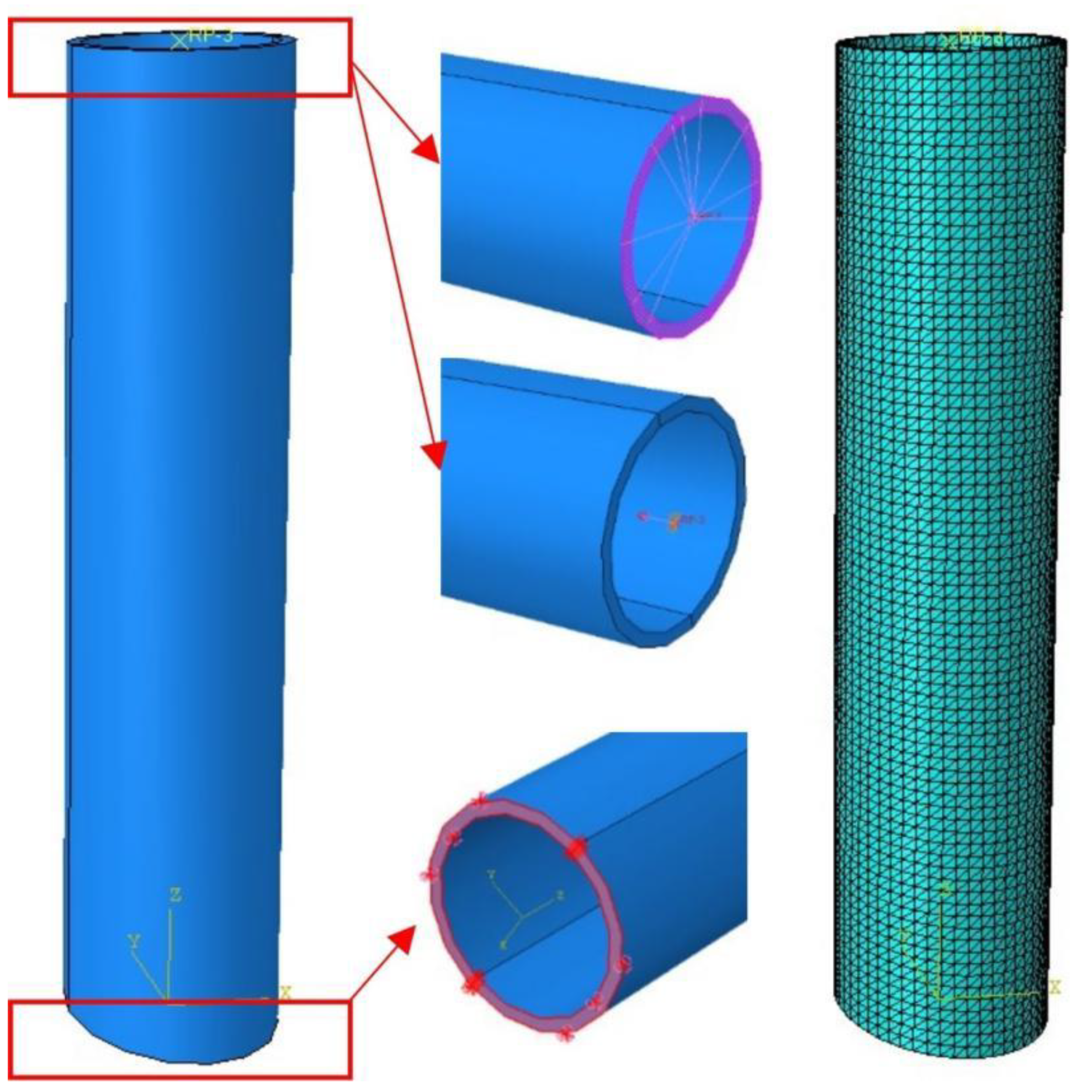
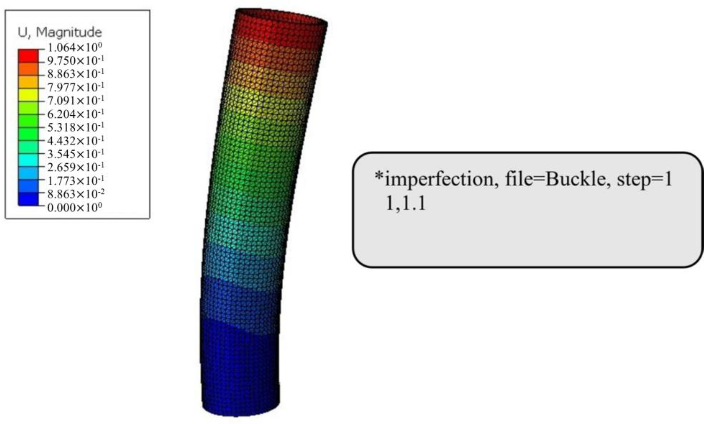
2.2. Finite Element Modeling
3. Mechanical Properties
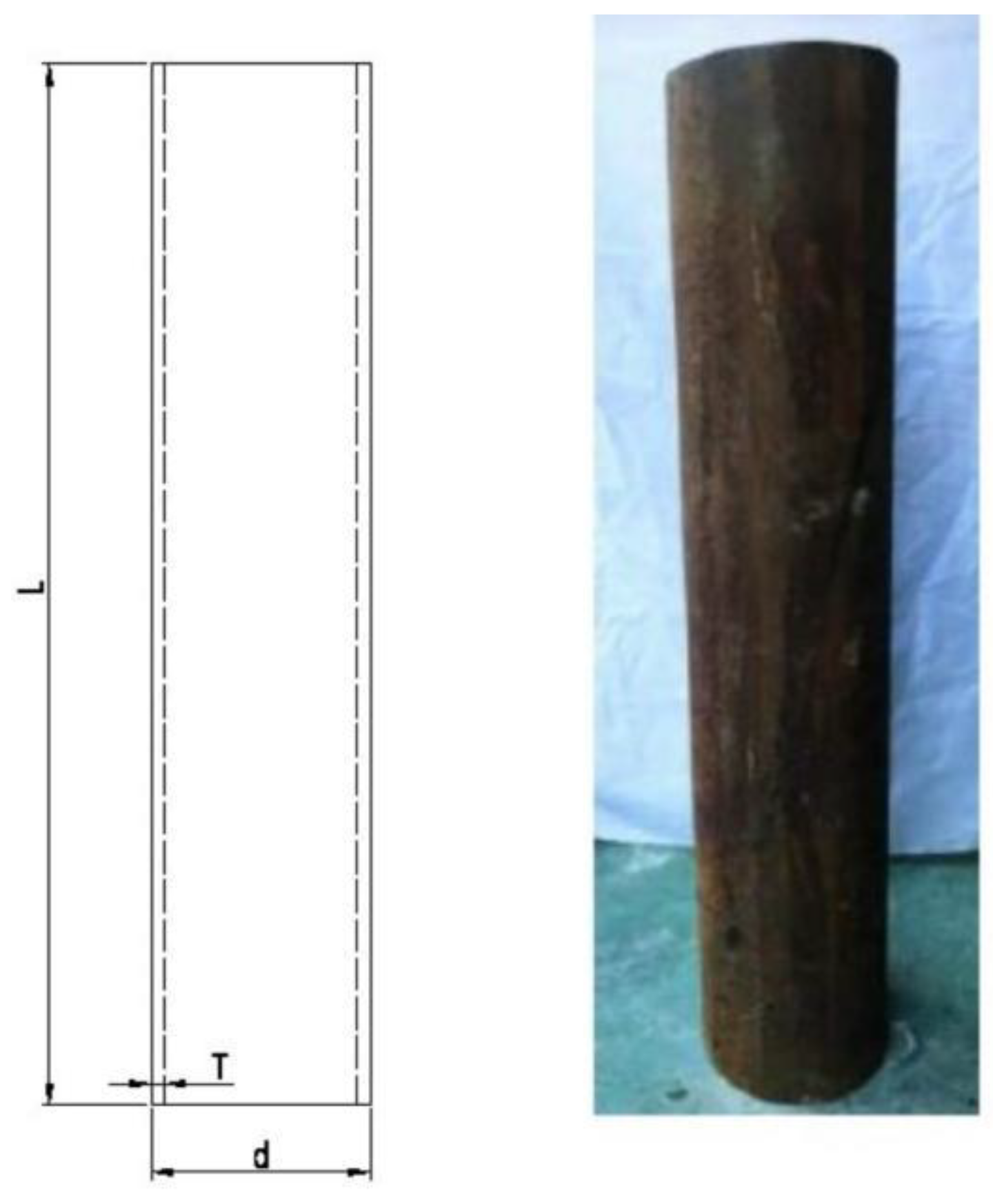
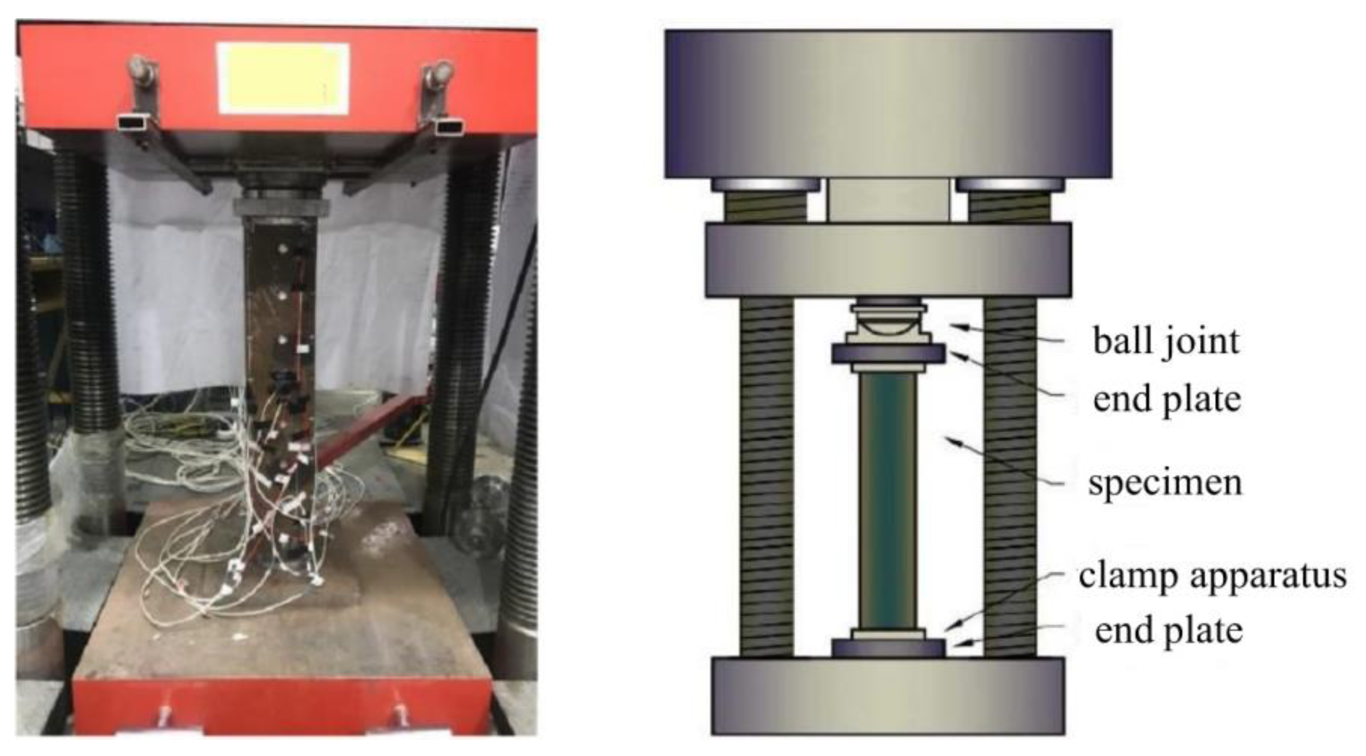
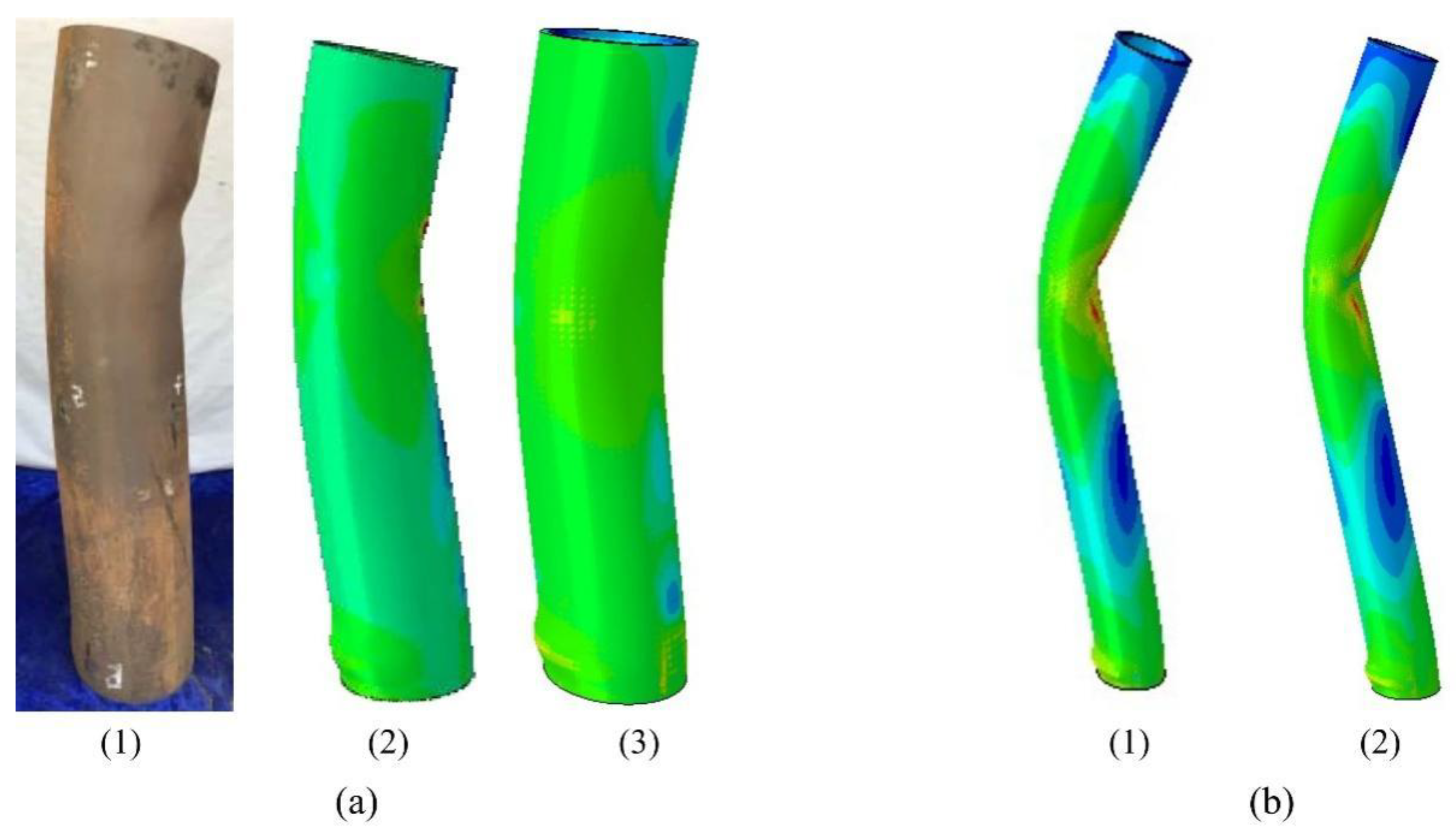
3.1. Experiment and FEM Analysis of Non-Pitting Specimens
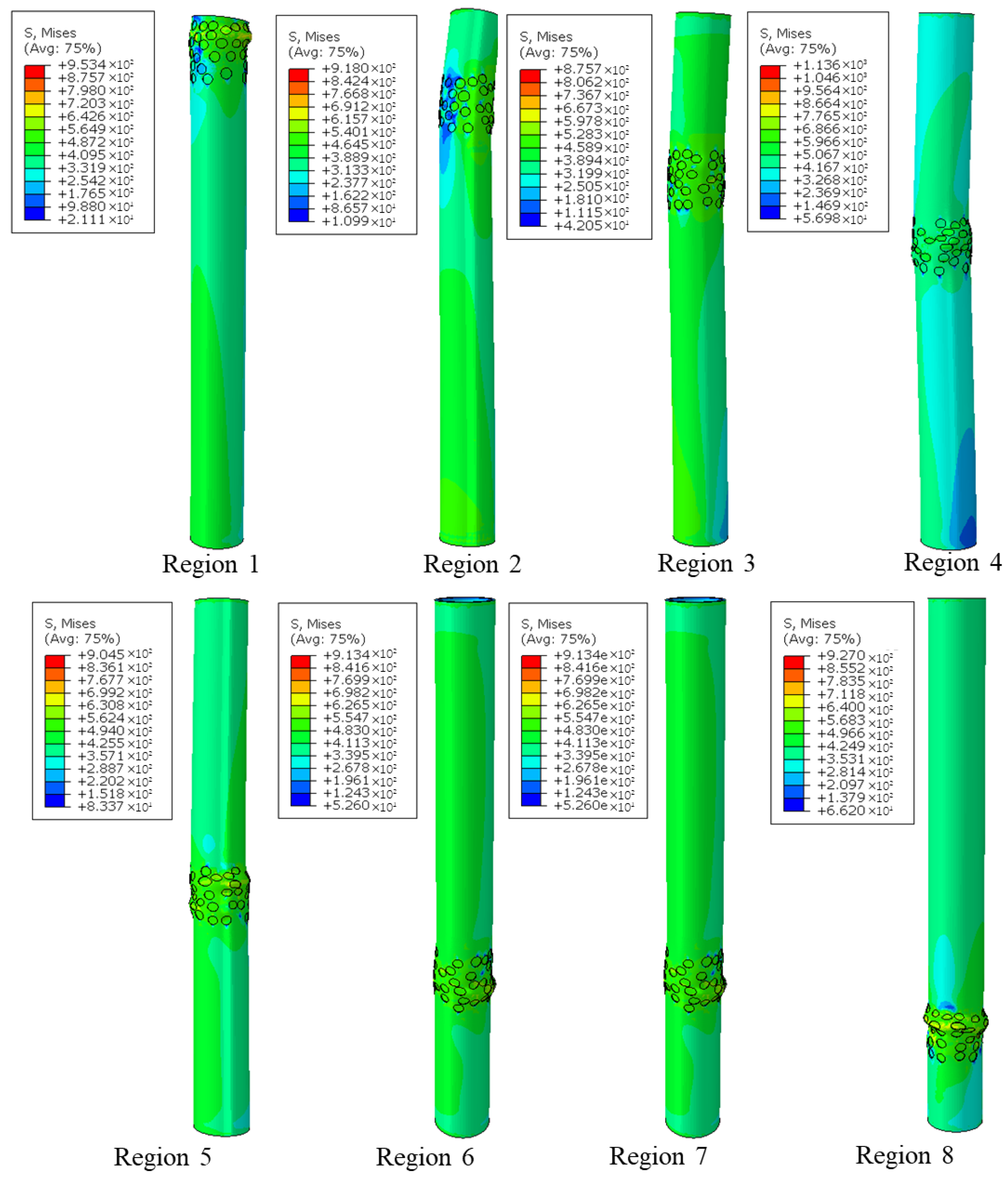
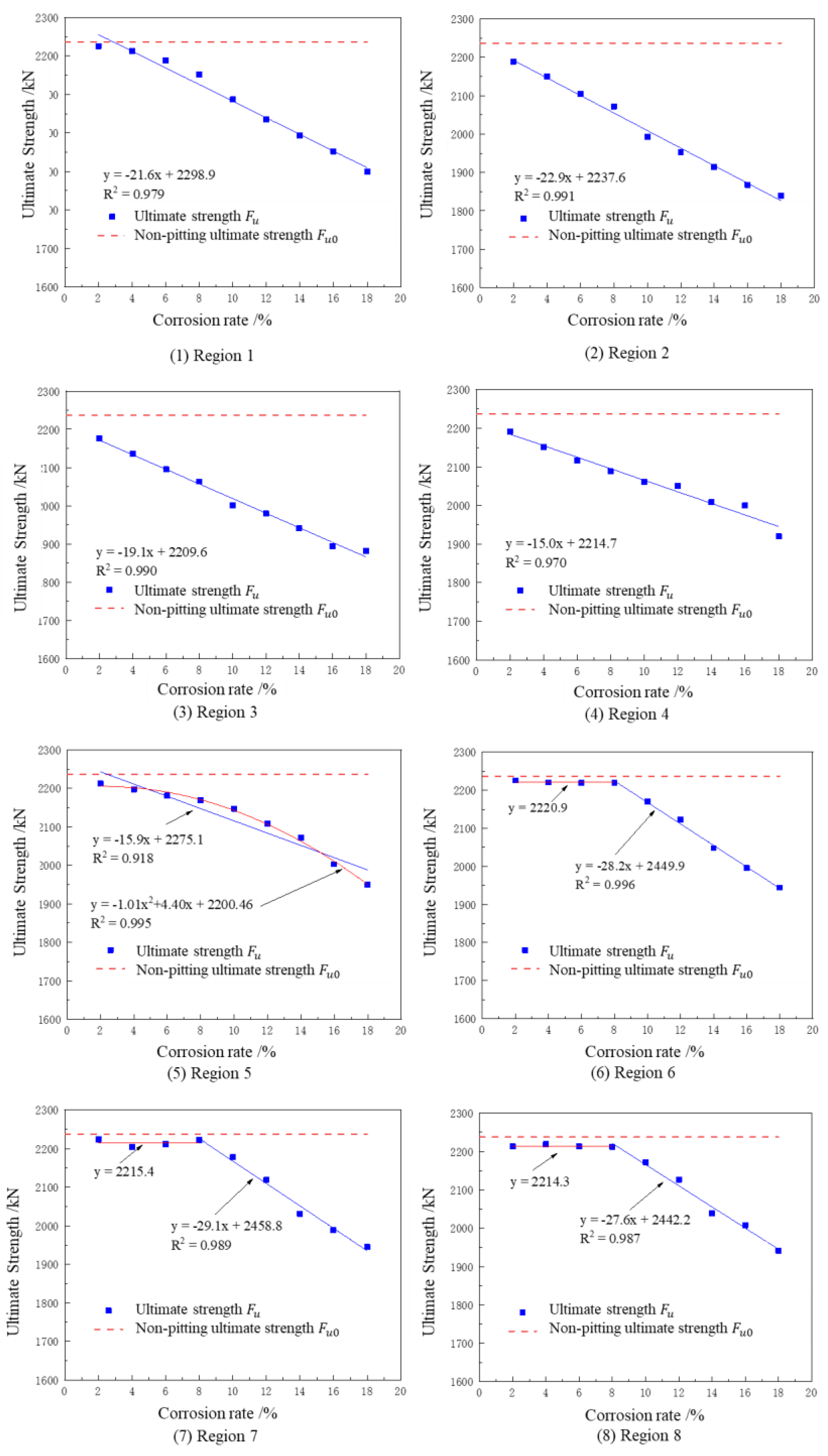
3.2. Influence of Local Random Pitting Rate
4. CNN for Pitting Detection
4.1. Critical Pitting Corrosion Rate
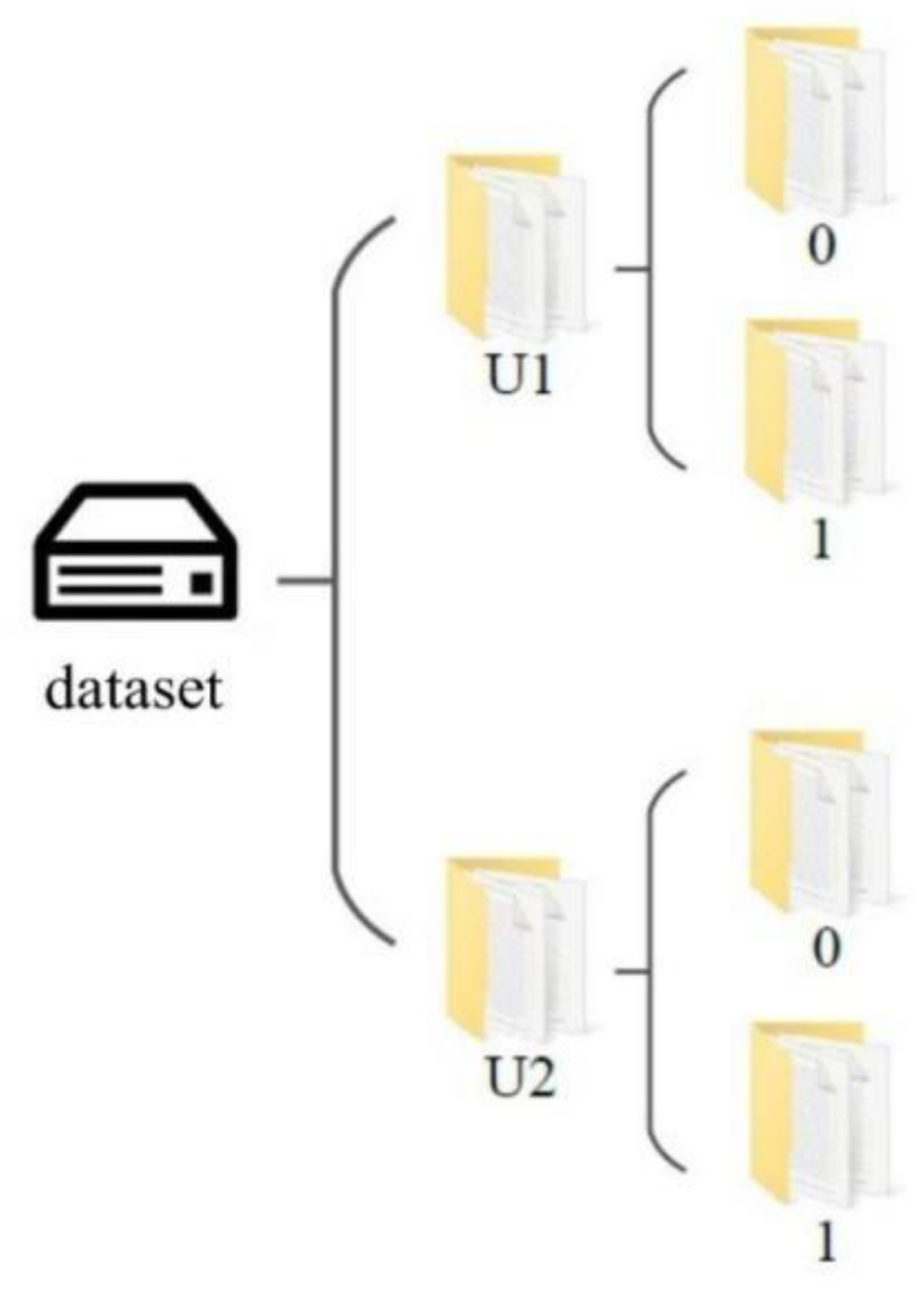
4.2. Dataset
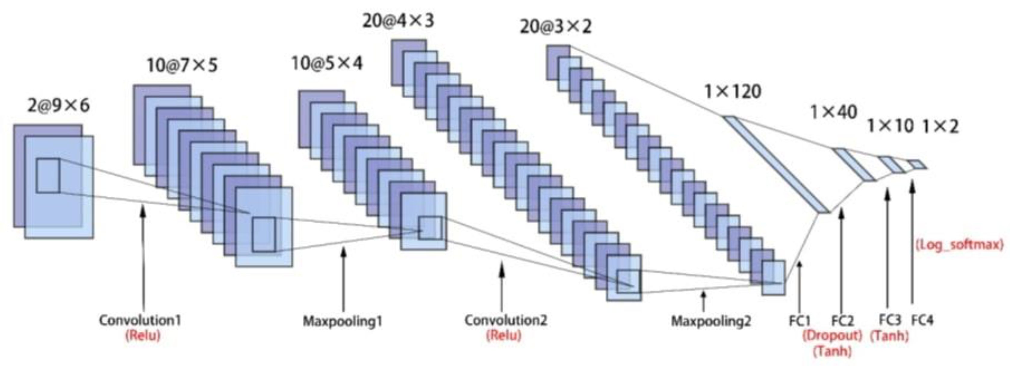
4.3. CNN
5. Results and Discussion
6. Conclusions
- (1)
- The accuracy of the numerical model. The multi-parameter localized random pitting numerical model established herein can fully express the randomness of pitting pits in shape and location while ensuring the reasonable shape parameters and location coordinates of pitting pits, which can fully describe the realistic pitting situation of steel columns.
- (2)
- Statistical patterns of bearing capacity of localized random pitting corrosion in steel columns. With low dispersion, the ultimate strength distribution of localized random pitting steel columns has good statistical significance. For steel columns with one end fixed and one end hinged, the ultimate strength decreases linearly with the increase in the pitting corrosion rate when pitting occurs in regions 1–4; the ultimate strength shows a secondary parabolic downward trend as the pitting corrosion rate increases when pitting occurs in region 5; the bearing capacity of the steel column first remains constant and then shows a linear decrease with the increase in corrosion rate when pitting occurs in regions 6–8.
- (3)
- A pitting detection neural network. This study establishes a convolutional neural network to determine whether a steel component is damaged or not by inputting the first six vibration modes. The network has a high detection accuracy, which meets the practical engineering requirements and proves that it is of great theoretical significance and actual application value to determine the damage to a steel component by the convolutional neural network.
- (4)
- The detection system of random pitting corrosion. Based on the numerical model of random pitting, the critical corrosion rate is defined by studying the ultimate strength of pitting components, and then vibration modes are input to train the convolutional neural network for damage determination; thus, a localized random pitting damage determination network with reasonable accuracy is worked out.
Author Contributions
Funding
Institutional Review Board Statement
Informed Consent Statement
Data Availability Statement
Conflicts of Interest
References
- Frankel, G.S. Pitting corrosion of metals—A review of the critical factors. J. Electrochem. Soc. 1998, 145, 2186–2198. [Google Scholar] [CrossRef]
- Peyre, P.; Scherpereel, X.; Berthe, L.; Carboni, C.; Fabbro, R.; Beranger, G.; Lemaitre, C. Surface modifications induced in 316L steel by laser peening and shot-peening. Influence on pitting corrosion resistance. Mater. Sci. Eng. A-Struct. Mater. Prop. Microstruct. Process. 2000, 280, 294–302. [Google Scholar] [CrossRef]
- Guedes Soares, C.; Garbatov, Y.; Zayed, A. Effect of environmental factors on steel plate corrosion under marine immersion conditions. Corros. Eng. Sci. Technol. 2011, 46, 524–541. [Google Scholar] [CrossRef]
- Velázquez, J.; van der Weide, H.; Hernandez-sÁNchez, E.; Hernández, H. Statistical Modelling of Pitting Corrosion: Extrapolation of the Maximum Pit Depth-Growth. Int. J. Electrochem. Sci. 2014, 9, 4129–4143. [Google Scholar] [CrossRef]
- Bhandari, J.; Khan, F.; Abbassi, R.; Garaniya, V.; Ojeda, R. Modelling of pitting corrosion in marine and offshore steel structures—A technical review. J. Loss Prev. Process Ind. 2015, 37, 39–62. [Google Scholar] [CrossRef]
- Pardo, A.; Merino, M.C.; Coy, A.E.; Viejo, F.; Arrabal, R.; Matykina, E. Pitting corrosion behaviour of austenitic stainless steels—Combining effects of Mn and Mo additions. Corros. Sci. 2008, 50, 1796–1806. [Google Scholar] [CrossRef]
- Shi, Y.; Yang, B.; Liaw, P.K. Corrosion-Resistant High-Entropy Alloys: A Review. Metals 2017, 7, 43. [Google Scholar] [CrossRef] [Green Version]
- Qiang, X.; Shen, Y.; Jiang, X.; Bijlaard, F.S.K. Theoretical study on initial stiffness of thin-walled steel T-stubs taking account of prying force. Thin-Walled Struct. 2020, 155, 106944. [Google Scholar] [CrossRef]
- Qiang, X.; Shu, Y.; Jiang, X. Experimental and numerical study on high-strength steel flange-welded web-bolted connections under fire conditions. J. Constr. Steel. Res. 2022, 192, 107255. [Google Scholar] [CrossRef]
- Qiang, X.; Wu, Y.; Wang, Y.; Jiang, X. Novel crack repair method of steel bridge diaphragm employing Fe-SMA. Eng. Struct. 2023, 292, 116548. [Google Scholar] [CrossRef]
- Jiang, X.; Guedes Soares, C. Ultimate capacity of rectangular plates with partial depth pits under uniaxial loads. Mar. Struct. 2012, 26, 27–41. [Google Scholar] [CrossRef]
- Jiang, X.; Guedes Soares, C. A closed form formula to predict the ultimate capacity of pitted mild steel plate under biaxial compression. Thin-Walled Struct. 2012, 59, 27–34. [Google Scholar] [CrossRef]
- Nakai, T.; Matsushita, H.; Yamamoto, N.; Arai, H. Effect of pitting corrosion on local strength of hold frames of bulk carriers (1st report). Mar. Struct. 2004, 17, 403–432. [Google Scholar] [CrossRef]
- Pidaparti, R.M.; Palakal, P.J.; Fang, L. Cellular automation approach to model aircraft corrosion pit damage growth. Aiaa J. 2004, 42, 2562–2569. [Google Scholar] [CrossRef]
- Miao, C.Q.; Yu, J.; Mei, M.X. Distribution law of corrosion pits on steel suspension wires for a tied arch bridge. Anti-Corros. Methods Mater. 2016, 63, 166–170. [Google Scholar] [CrossRef]
- Sharifi, Y. Reliability of deteriorating steel box-girder bridges under pitting corrosion. Adv. Steel Constr. 2011, 7, 220–238. [Google Scholar]
- Zhang, X.Z.; Liu, R.; Chen, K.Y.; Yao, M.X. Pitting Corrosion Characterization of Wrought Stellite Alloys in Green Death Solution with Immersion Test and Extreme Value Analysis Model. J. Mater. Eng. Perform. 2014, 23, 1718–1725. [Google Scholar] [CrossRef]
- Ossai, C.I.; Boswell, B.; Davies, I. Markov chain modelling for time evolution of internal pitting corrosion distribution of oil and gas pipelines. Eng. Fail. Anal. 2016, 60, 209–228. [Google Scholar] [CrossRef] [Green Version]
- Rivas, D.; Caleyo, F.; Valor, A.; Hallen, J.M. Extreme value analysis applied to pitting corrosion experiments in low carbon steel: Comparison of block maxima and peak over threshold approaches. Corros. Sci. 2008, 50, 3193–3204. [Google Scholar] [CrossRef]
- Melchers, R.E. Pitting corrosion of mild steel in marine immersion environment-Part 2: Variability of maximum pit depth. Corrosion 2004, 60, 937–944. [Google Scholar] [CrossRef]
- Wang, Y.; Wharton, J.A.; Shenoi, R.A. Ultimate strength analysis of aged steel-plated structures exposed to marine corrosion damage: A review. Corros. Sci. 2014, 86, 42–60. [Google Scholar] [CrossRef]
- Sultana, S.; Wang, Y.; Sobey, A.J.; Wharton, J.A.; Shenoi, R.A. Influence of corrosion on the ultimate compressive strength of steel plates and stiffened panels. Thin-Walled Struct. 2015, 96, 95–104. [Google Scholar] [CrossRef]
- Cawley, P.; Adams, R.D. The location of defects in structures from measurements of natural frequencies. J. Strain Anal. Eng. Des. 1979, 14, 49–57. [Google Scholar] [CrossRef]
- Salawu, O.S. Detection of structural damage through changes in frequency: A review. Eng. Struct. 1997, 19, 718–723. [Google Scholar] [CrossRef]
- Xiao, F.; Meng, X.; Zhu, W.; Chen, G.; Yan, Y. Combined Joint and Member Damage Identification of Semi-Rigid Frames with Slender Beams Considering Shear Deformation. Buildings 2023, 13, 1631. [Google Scholar] [CrossRef]
- Xiao, F.; Zhu, W.; Meng, X.; Chen, G. Parameter Identification of Structures with Different Connections Using Static Responses. Appl. Sci. 2022, 12, 5896. [Google Scholar] [CrossRef]
- Pandey, A.K.; Biswas, M.; Samman, M.M. Damage detection from changes in curvature mode shapes. J. Sound Vib. 1991, 145, 321–332. [Google Scholar] [CrossRef]
- Wang, S.; Li, H.-J. Assessment of structural damage using natural frequency changes. Acta Mech. Sin. 2012, 28, 118–127. [Google Scholar] [CrossRef]
- Zhang, X.W.; Zhao, S.L.; Wang, Z.; Li, J.X.; Qiao, L.J. The pitting to uniform corrosion evolution process promoted by large inclusions in mooring chain steels. Mater. Charact. 2021, 181, 12. [Google Scholar] [CrossRef]
- Xiao, F.; Sun, H.; Mao, Y.; Chen, G. Damage Identification of Large-Scale Space Truss Structures Based on Stiffness Separation Method. Structures 2023, 53, 109–118. [Google Scholar] [CrossRef]
- Ben Seghier, M.E.; Keshtegar, B.; Taleb-Berrouane, M.; Abbassi, R.; Trung, N.T. Advanced intelligence frameworks for predicting maximum pitting corrosion depth in oil and gas pipelines. Process Saf. Environ. Protect. 2021, 147, 818–833. [Google Scholar] [CrossRef]
- Ossai, C.I. A Data-Driven Machine Learning Approach for Corrosion Risk Assessment—A Comparative Study. Big Data Cogn. Comput. 2019, 3, 28. [Google Scholar] [CrossRef] [Green Version]
- Sasidhar, K.N.; Siboni, N.H.; Mianroodi, J.R.; Rohwerder, M.; Neugebauer, J.; Raabe, D. Deep learning framework for uncovering compositional and environmental contributions to pitting resistance in passivating alloys. NPJ Mater. Degrad. 2022, 6, 10. [Google Scholar] [CrossRef]
- Sharifi, Y.; Tohidi, S. Ultimate capacity assessment of web plate beams with pitting corrosion subjected to patch loading by artificial neural networks. Adv. Steel Constr. 2014, 10, 325–350. [Google Scholar]
- Ossai, C.I. Corrosion defect modelling of aged pipelines with a feed-forward multi-layer neural network for leak and burst failure estimation. Eng. Fail. Anal. 2020, 110, 15. [Google Scholar] [CrossRef]
- Barai, S.V.; Pandey, P.C. Vibration Signature Analysis Using Artificial Neural Networks. J. Comput. Civ. Eng. 1995, 9, 259–265. [Google Scholar] [CrossRef]
- Qiao, Y.X.; Xu, D.K.; Wang, S.; Ma, Y.J.; Chen, J.; Wang, Y.X.; Zhou, H.L. Effect of hydrogen charging on microstructural evolution and corrosion behavior of Ti-4Al-2V-1Mo-1Fe alloy. J. Mater. Sci. Technol. 2021, 60, 168–176. [Google Scholar] [CrossRef]
- Cha, Y.J.; Choi, W.; Suh, G.; Mahmoudkhani, S.; Buyukozturk, O. Autonomous Structural Visual Inspection Using Region-Based Deep Learning for Detecting Multiple Damage Types. Comput.-Aided Civ. Infrastruct. Eng. 2018, 33, 731–747. [Google Scholar] [CrossRef]
- Chun, P.; Yamane, T.; Izumi, S.; Kameda, T. Evaluation of Tensile Performance of Steel Members by Analysis of Corroded Steel Surface Using Deep Learning. Metals 2019, 9, 1259. [Google Scholar] [CrossRef] [Green Version]
- Gupta, R.D.; Kundu, D. Generalized exponential distributions. Aust. N. Z. J. Stat. 1999, 41, 173–188. [Google Scholar] [CrossRef]
- Wallace, J.; Reddy, R.; Pugh, D.; Pacheco, J. Sour Service Pit Growth Predictions of Carbon Steel using Extreme Value Statistics. In Proceedings of the CORROSION 2007, Nashville, TN, USA, 11–15 March 2007. [Google Scholar]
- Keliang, R.E.N.; Guozhi, L.U.; Yohong, Z. Stochastic Arrange and Computer Simulation of Corrosion Pitting in Damage Structure. Acta Aeronaut. Et Astronaut. Sin. 2006, 27, 459–462. [Google Scholar]
- Wang, Y.W.; Wu, X.Y.; Zhang, Y.H.; Huang, X.P.; Cui, W. Pitting corrosion model of mild and low-alloy steel in marine environment-Part 2: The shape of corrosion pits. J. Ship Mech. 2007, 11, 735–743. [Google Scholar]
- Qin, J.Y. Study on Mechanical Properties of Marine Steel Pipe considering Pitting Damage. Master’s Thesis, Dalian University of Technology, Dalian, China, 2020. [Google Scholar]
- GB50017-2017; Standard for Design of Steel Structures. Ministry of Housing and Urban-Rural Development: Beijing, China, 2017.


| Slenderness Ratio ζ | Length L/mm | Thickness T/mm | Diameter d/mm | Section Length s/mm |
|---|---|---|---|---|
| 20 | 1309 | 10 | 168.3 | L/8 |
| 25 | 1636 | |||
| 30 | 1964 | |||
| 35 | 2291 |
| Parameter | Unit | Illustration |
|---|---|---|
| mm | Length of specimen | |
| mm | Diameter of specimen | |
| mm | Thickness | |
| % | Number of regions | |
| % | Corrosion rate | |
| t | year | Corrosion time |
| - | Initial pit number |
| t | |
|---|---|
| 7 | 0.02,0.04,0.06,0.08 |
| 9 | |
| 11 | |
| 15 | 0.10,0.12,0.14,0.16,0.18 |
| 20 | |
| 25 | |
| 30 | |
| 35 | |
| 40 |
| 2.38 × 10⁵ | 0.3 | 8.104 × 10⁻⁹ | 460 | 555 |
| Experimental Result | Qin’s FE Result | FEM Result | Error 1 | Error 2 | |
|---|---|---|---|---|---|
| 12.22 | 2424 | 2384.3 | 2446.1 | 0.90% | 2.60% |
| 25 | - | 2315.6 | 2237.2 | - | 3.40% |
| Layer Name | Number of Filters | Size or Dropout Rate | Output Size |
|---|---|---|---|
| Input layer | - | - | 2 × 9 × 6 |
| Convolution layer 1 | 10 | 3 × 2 | 10 × 7 × 5 |
| Max-pooling layer 1 | - | 3 × 2 | 10 × 5 × 4 |
| Convolution layer 2 | 20 | 2 × 2 | 20 × 4 × 3 |
| Max-pooling layer 2 | - | 2 × 2 | 20 × 3 × 2 |
| Fully connected layer 1 | - | - | 1 × 120 |
| Dropout | - | 0.3 | - |
| Fully connected layer 2 | - | - | 1 × 40 |
| Fully connected layer 3 | - | - | 1 × 10 |
| Output layer | - | - | 1 × 2 |
Disclaimer/Publisher’s Note: The statements, opinions and data contained in all publications are solely those of the individual author(s) and contributor(s) and not of MDPI and/or the editor(s). MDPI and/or the editor(s) disclaim responsibility for any injury to people or property resulting from any ideas, methods, instructions or products referred to in the content. |
© 2023 by the authors. Licensee MDPI, Basel, Switzerland. This article is an open access article distributed under the terms and conditions of the Creative Commons Attribution (CC BY) license (https://creativecommons.org/licenses/by/4.0/).
Share and Cite
Jiang, X.; Qi, H.; Qiang, X.; Zhao, B.; Dong, H. A Convolutional Neural Network-Based Corrosion Damage Determination Method for Localized Random Pitting Steel Columns. Appl. Sci. 2023, 13, 8883. https://doi.org/10.3390/app13158883
Jiang X, Qi H, Qiang X, Zhao B, Dong H. A Convolutional Neural Network-Based Corrosion Damage Determination Method for Localized Random Pitting Steel Columns. Applied Sciences. 2023; 13(15):8883. https://doi.org/10.3390/app13158883
Chicago/Turabian StyleJiang, Xu, Hao Qi, Xuhong Qiang, Bosen Zhao, and Hao Dong. 2023. "A Convolutional Neural Network-Based Corrosion Damage Determination Method for Localized Random Pitting Steel Columns" Applied Sciences 13, no. 15: 8883. https://doi.org/10.3390/app13158883