Path Planning of Rail-Mounted Logistics Robots Based on the Improved Dijkstra Algorithm

Featured Application

The improved Dijkstra algorithm proposed herein can be effectively applied to rail-mounted robots to distribute goods in large workshops, especially in ultra-clean semiconductor chip production workshops. The algorithm can plan the shortest route for the robots to distribute goods, adjust to conflicts in real time, and complete multiple distribution tasks for multiple robots.

Abstract

With the upgrading of manufacturing production lines and innovations in information technology, logistics robot technology applied in factories is maturing. Rail-mounted logistics robots are suitable for precise material distribution in large production workshops with fixed routes and over long distances. However, designing an efficient path-planning algorithm is the key to realizing high efficiency in multi-robot system operations with rail logistics. Therefore, this paper proposes an improved Dijkstra algorithm that introduces real-time node occupancy and a time window conflict judgment model for global path planning and conflict coordination in multi-robot systems. More specifically, the introduction of real-time node occupancy can determine the shortest feasible routes for each task, and the introduction of the time window conflict judgment model can avoid the route conflict problem in the execution of multiple tasks, planning the shortest route without conflict. For the robot UBW positioning module, a Chan algorithm based on TDOA is proposed to realize the accurate positioning of rail-mounted logistics robots during their operation. Compared with the traditional Dijkstra algorithm, the results show that the algorithm proposed herein can plan a conflict-free and better path and dynamically adjust the on-orbit conflict in real time to avoid track congestion and efficiently complete multiple distribution tasks.

1. Introduction

Rail-mounted logistics robots are suitable for complex material distributions in large production workshops with fixed routes and long distances. The goal of robot path planning is to find the shortest path from the starting point to the target point without conflict. The application scenario of this paper is for large-scale workshop material distribution, especially in ultra-clean semiconductor chip production workshops. The walkable track of the logistics robot is laid on the top of the workshop, and the robot can reach all the cargo stations and workstations in the workshop along the track. When each workstation needs a certain material, it passes the out-of-stock information to the system. After receiving multiple out-of-stock notifications, the system starts the robot from the material station, distributes the goods to the corresponding workstation along the track, and then returns to the goods station. There may be one or more cargo stations inside the workshop. Based on the calculation of the optimization algorithm, multiple logistics robots cooperate to complete all the material delivery tasks, which can reduce labor costs and improve the efficiency of material delivery to a large extent. However, overlapping path regions occur when multiple robots perform distribution tasks along the track. Therefore, to avoid robot on-orbit conflicts and invalid waiting, we need to consider the coordination method for robot on-orbit conflicts.

In the field of computer science, according to the definition of the deterministic Turing machine model and non-deterministic Turing machine model, the traveling salesman problem (TSP), graph coloring problem (GCP), vertex cover, and other classical problems are defined as non-deterministic polynomial problems (NP), NP-hard (NPH), and NP-complete (NPC) [1,2]. A problem is said to be NP-hard if all the NP-class problems are reduced to a single problem. NP-hard problems are more general than NP-complete problems, and it is difficult to find exact solutions in polynomial time.

The resources in this paper include the number of parallel tracks, payloads, and robots. The MD-MTSP problem dealt with by the algorithm proposed in this paper has discrete time, and it is relatively easy to find a feasible solution within the resource condition, but the optimal solution is almost impossible to find within an acceptable time. However, beyond the resource conditions, it is an NP-hard problem, which cannot be solved in polynomial time.

In this paper, the path-planning problem of the rail-mounted logistics robot is modeled as a multi-depot multiple traveling salesman problem (MD-MTSP); that is, the robot is abstracted as a traveling salesman, and the material station and work station are abstracted as a city. A number of traveling salesmen depart from many different cities, each of which must be visited by at least one salesman, and only once, except for the origin and destination cities. Under this condition, the shortest path traversing all the cities is found. The multi-depot multiple traveling salesman problem is a kind of multiple traveling salesman problem. The multiple traveling salesman problem is an extension of the famous traveling salesman problem (TSP). It is an NP-hard problem and has a strong engineering background and application value.

The commonly used path planning algorithms include the A* algorithm [3,4], Dijkstra algorithm [5,6], particle swarm optimization (PSO) [7], Floyd algorithm [6], PRM algorithm [7], RRT algorithm [8], genetic algorithm (GA) [8,9,10], and ant colony optimization (ACO) [11,12]. These methods should be further improved when considering the path allocation, energy allocation, and global shortest path, thereby ensuring the robustness and fault tolerance of the multi-machine system.

PSO, GA, and ACO are heuristic algorithms, which generally have shortcomings, including susceptibility to falling into a local optimum, premature convergence, and limited scope of application. GA is based on natural selection and heredity, producing optimal solutions from the previous generation. Recently, Abdel-Nasser Sharkawy’s team [13] used a genetic algorithm to find the high-performance position of a task with the goal of realizing the efficient collaborative operation of a human arm and a robotic arm. Although the genetic algorithm has been widely used to solve MTSP, most of the solutions involve transforming MTSP into TSP. The focus of this research is on how to express MTSP via chromosome coding, and how to improve the genetic algorithm by changing the chromosome coding method. Due to the limitation of its improvement method, the role that the genetic algorithm can play in solving this problem is limited.

The A* and Dijkstra algorithms are graph search algorithms that directly find a path in a graph. The A* algorithm is a heuristic search algorithm, which needs to decompose the operating environment into raster data during the working process for computing the cost function. However, the A* algorithm has high requirements for the operating environment of a robot, and when the operating environment is complex, this decomposition takes a long time. Additionally, when the running environment changes, the decomposition needs to be done again, which affects the efficiency of the A* algorithm.

Among these, Edsger Wybe Dijkstra’s method [14] is a traditional approach that was put forth in 1956 to address the problem of finding the shortest path between any two points on a map. Dijkstra’s algorithm, which has been used extensively to solve the optimal path issue [15,16], has the advantages of a simple structure, good convergence, and high practicability compared to Floyd’s algorithm, the A* algorithm, and other global path planning algorithms. The efficiency of the technique is extremely low because it must explore every point in space, which requires a significant amount of computation and memory. Numerous complicated issues, including navigational lines, dynamic planning, logistics scheduling, etc., can be resolved by improving and optimizing Dijkstra’s algorithm.

Sunita et al. [17] improved Dijkstra’s algorithm by using the traceable priority queue data structure to achieve dynamic and effectively reduce the running time and running memory, but the performance of the solution may be somewhat less than the best resource bounds known so far. Huang Yihu et al. [18] enhanced Dijkstra’s algorithm by adding a time window conflict judgment model, which is appropriate for multi-robot path planning and may avoid conflicts. In order to achieve the shortest distance and shortest time path planning for AGV (Automated Guided Vehicle) under rectangular environment graphs, Qing Guo et al. [19] suggested an improved Dijkstra method with the addition of running time. In order to accelerate the path-planning process, Zhou et al. [20] integrated the ant colony method and Dijkstra’s algorithm for the airport AGV path-planning scenario. Durakli et al. [21] modified the Dijkstra method by including the Bezier curve to realize route optimization, made the path smoother, and could track the obstacles in the way in real time and update the path. They performed this while taking into account the continuity of the path. To address the fuzzy shortest path problem in graphics, Akram et al. [22] suggested an adaptive Dijkstra method based on trapezoidal image blur numbers. The dynamic window algorithm (DWA) and Dijkstra’s algorithm were integrated by Liu et al. [23] and applied to intelligent cars, which performed well in path-planning navigation and obstacle avoidance.

Additionally, the traditional Dijkstra method can be used for network communication’s shortest route selection, but not for paths with limited resources or continuity. In the context of optical networks, Ireneusz Szczesniak et al. [24] recently proposed a general Dijkstra algorithm that effectively finds the shortest path using a network of discrete resources with continuity and continuity requirements. Ireneusz Szczesniak and colleagues rectified the flaw of the general Dijkstra algorithm, which only sorted the tags in the priority queue according to the ascending order of cost, and demonstrated the soundness of the method by induction by introducing the Bellman optimality principle.

While our current research and the work conducted by Ireneusz et al. both aim to enhance the traditional Dijkstra algorithm and utilize it for the purpose of finding the shortest path, it is important to note that the approaches employed and the specific contexts in which they are applied differ. Currently, we propose the implementation of a real-time occupancy and time window conflict judgment model for each site. This model addresses the limitation of the traditional Dijkstra algorithm, which does not account for the time factor. Additionally, it enables multi-robot on-orbit anti-collision capabilities, thereby enhancing the efficiency of the algorithm. Ireneusz et al. proposed an enhancement of the Dijkstra algorithm that addresses the limitation of the traditional Dijkstra algorithm in searching for the shortest path in networks with discrete resources and continuous constraints [24].

Ultrawideband (UWB) positioning technology encompasses many methods that can be categorized based on distinct positioning criteria, namely Time Difference of Arrival (TDOA), Time of Arrival (TOA), and Angle of Arrival (AOA). The Chan method and Taylor algorithm are two well-established location algorithms that rely on Time Difference of Arrival (TDOA) measurements. The Chan algorithm aims to determine the posterior probability distribution function with the highest value, whereas the Taylor algorithm is computed based on the Hessian matrix. The approach proposed by Chan, which utilizes the Time Difference of Arrival (TDOA), has gained significant popularity because of its computational efficiency and superior location accuracy [25].

This study utilizes the enhanced Dijkstra algorithm to address the challenges associated with global path planning and conflict coordination in a multi-robot system. The efficiency of the traditional Dijkstra algorithm can be enhanced by addressing the limitation of disregarding the time component through the introduction of the node real-time occupancy and time window judgment conflict model. The enhanced Dijkstra algorithm, which incorporates real-time node occupancy, enables the identification of all feasible shortest routes across various tasks. Additionally, the integration of the time window conflict judgment model mitigates route conflicts during the execution of multiple tasks, facilitating the planning of conflict-free shortest routes. Simultaneously, an innovative algorithm utilizing the Time Difference of Arrival (TDOA) and Channel (Chan) is implemented to enable real-time positioning of rail-mounted logistics robots within the workshop. The algorithm presented in this study aims to optimize path planning for multiple robots in large workshops, with the objectives of minimizing travel distance, reducing travel time, and minimizing the number of turns. Additionally, the algorithm is designed to effectively handle conflicts and efficiently complete multiple distribution tasks. The ultimate goal is to achieve automation and unmanned operations in material distribution within these large workshop settings.

2. Materials and Methods

In this section, we analyze the steps of the traditional Dijkstra algorithm and specifically how to improve it. In order to prevent conflicts between robots more effectively, we formulate priority rules and coordination methods when encountering conflicts. In addition, the robot UWB positioning module uses the Chan algorithm based on TDOA, which has better performance than the Taylor algorithm.

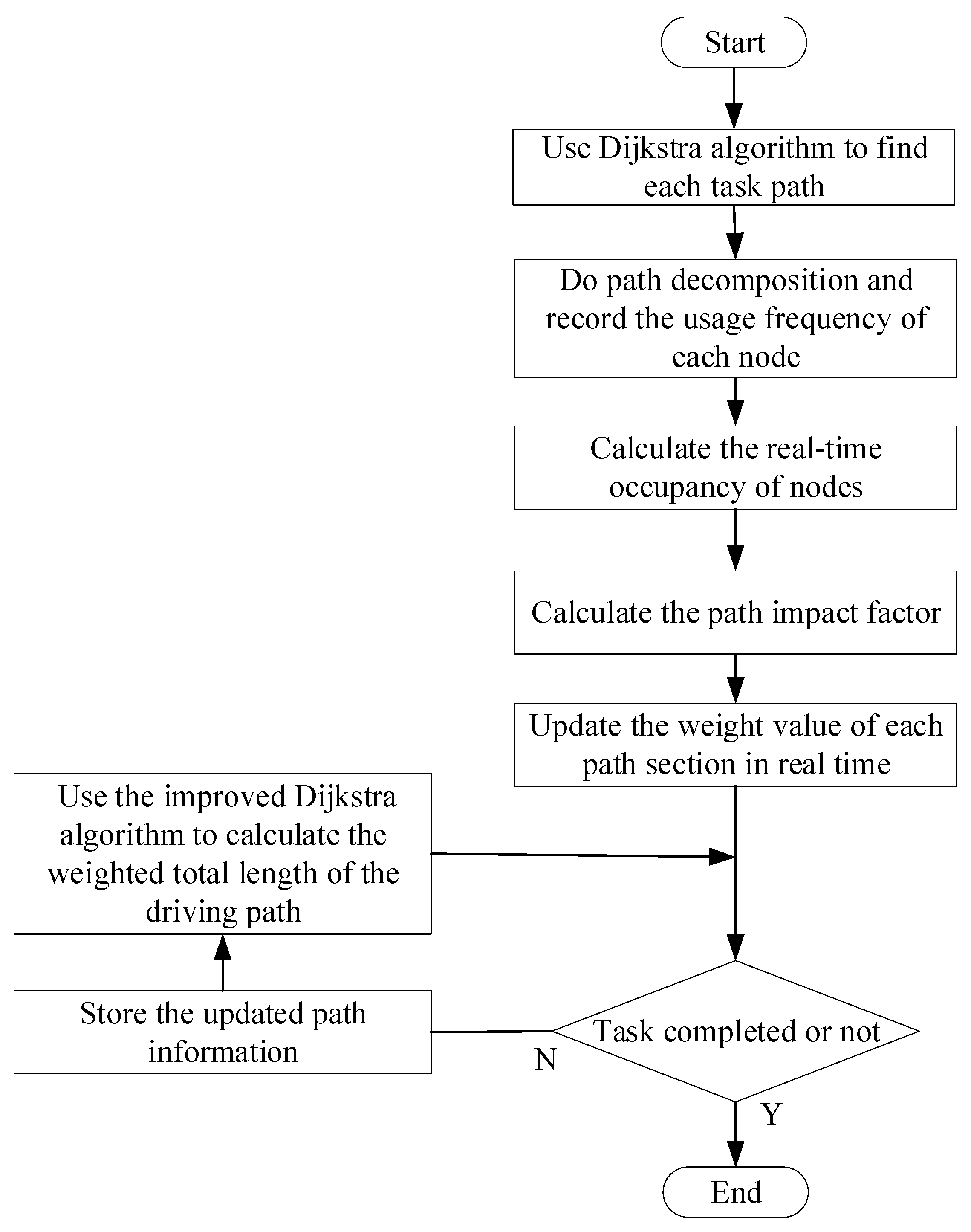
2.1. The Improved Dijkstra Algorithm

2.1.1. Dijkstra Algorithm Analysis

The fundamental concept underlying Dijkstra’s algorithm is that of a greedy algorithm. This procedure involves selecting a designated starting point and generating an array that captures the shortest distances from this starting point to all other points. Subsequently, the algorithm iteratively identifies the closest point to the current position, updates the current point to the closest point, and recalculates the distances from the starting point through the current point to all other points. This process continues until the shortest distance data are updated appropriately. The selected points are those that are identified as determining the shortest path and are not included in subsequent calculations. The ultimate outcome is the most concise route from the initial location to each of the remaining nodes.

The flow of the traditional Dijkstra’s algorithm is as follows:

• Define the set sum $S$ and $H$, perform initialization, let $S=\left\{V_0\right\}$
  where $S$ is the shortest path target node set, $H$ is the set of nodes excluding $S$, $V0$ is the initial node, and $VP$ is the target node.
• Select the node $Vk$ closest to the initial node $V0$ in set $H$, so that

  $$L\left[V_m,V_n\right]=\mathit{min}\left\{L\left[V_m,V_k\right]+L\left[V_k,V_n\right]\right\}$$

  (1)

  where $L\left[V_m,V_n\right]$ is the distance matrix, and then the distance between any two nodes can be expressed as

  $$L\left[V_m,V_n\right]=l_{mn}(m,n=\mathrm{1,2},3\cdots )$$

  (2)
• Update set $S$ and $H$ as

  $$S=S+\left\{V_k\right\},\hspace{1em}{V}_k\in H$$

  (3)

  $$H=H-\left\{V_k\right\},\hspace{1em}{V}_k\in H$$

  (4)
• Correct path length if

  $$L\left[V_m,V_n\right]>L\left[V_m,V_k\right]+L\left[V_k,V_n\right]$$

  (5)
  Then, L is amended as

  $$L\left[V_m,V_n\right]=L\left[V_m,V_k\right]+L\left[V_k,V_n\right]$$

  (6)
• Judge whether all the target nodes are added to the shortest path set $S$; if not, jump to step 2; otherwise, output the shortest path node set $S$.

The traditional Dijkstra algorithm has the disadvantage of ignoring the time factor and is prone to in-orbit conflicts. To solve this problem, the real-time occupation of the site is introduced into the path weight function of the Dijkstra algorithm.

2.1.2. Introducing the Real-Time Node Occupancy into Dijkstra’s Algorithm

The steps are as follows:

1.

The traditional Dijkstra algorithm is used to plan the initial distribution path for the robot, and the initial distribution path is decomposed in real time. The driving frequency $K_{V_i}$ of each robot on each node is recorded, and the real-time occupancy of this node is calculated according to

$$f\left(V_i\right)=K_{V_i}/\sum ^{\underset{p}{k=0}}{K}_{V_k}$$

(7)

2.

The real-time node occupancy is introduced into the weight function of the traditional Dijkstra algorithm, and the impact factor and real-time node occupancy of the traditional Dijkstra algorithm are considered at the same time. In this case, the weight function of Dijkstra’s algorithm is as follows:

$$L^{\prime }\left(V_0,V_p\right)=\sum ^{\underset{p}{i=0}}(1+f(V_i))\cdot L\left(V_0,V_p\right)$$

(8)

where the initial factor of the path node is 1, $L\left(V_0,V_p\right)$ is the original length of the path, and $L^{\prime }\left(V_0,V_p\right)$ is the weight after considering the real-time occupancy of the node.

The process of Dijkstra’s algorithm considering the real-time occupation of the nodes is shown in Figure 1:

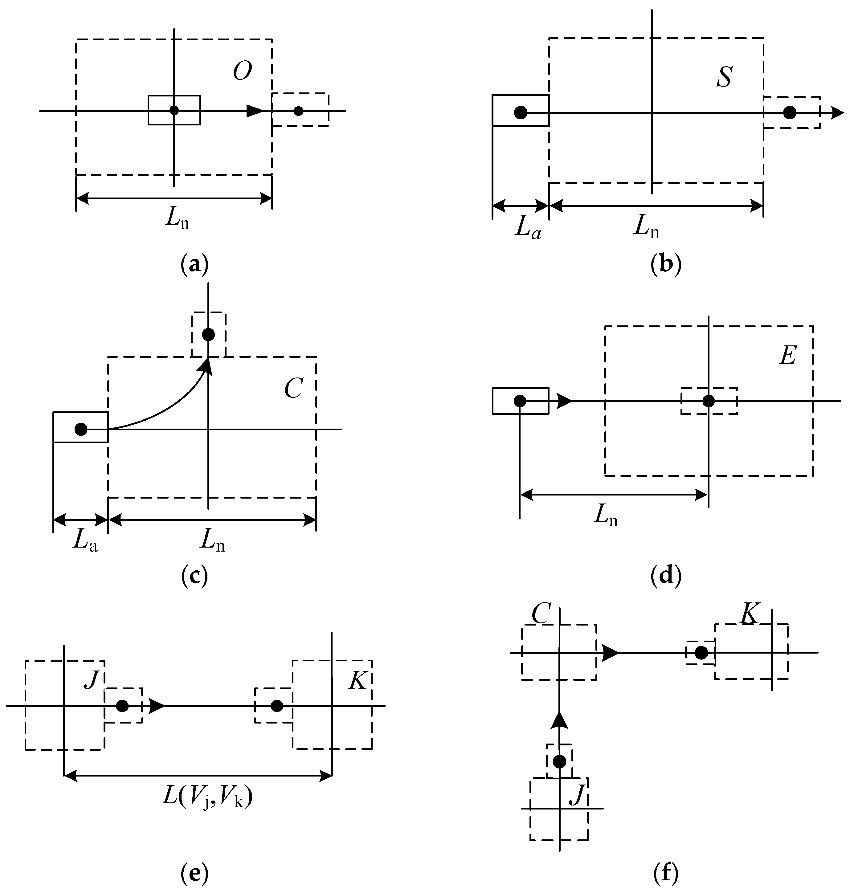
2.1.3. Introducing the Time Window Model into Dijkstra’s Algorithm

In order to carry out path planning for multiple rail-mounted logistics robots in a global dynamic environment, the time window model [26] is introduced. The time from entering a station to leaving the station is taken as the time window of the station.

The time window model is specified as follows:

• The traveling speed of the robot in orbit is 1 m/s;
• The maximum number of on-orbit robots in the same section of the track is 4;
• The start and stop times and reversing time of the robot are not considered;
• Each station can only be entered by one robot at the same time, and the other robots can only enter after occupying the right to contact.

The established time window model is as follows:

$$T_i=\left\{t_i=\left[t_i^{\mathrm{in}},t_i^{\mathrm{out}}\right]\right\}$$

(9)

where $Ti$ is the time window occupied by the I-th site, $t_i$ is the time window occupied by site $V_i$, $t_i^{\mathrm{out}}$ is the start time of the time window, and $t_i^{\mathrm{in}}$ is the end time of the time window.

Assuming that the linear speed of the rail-mounted logistics robot in the orbit is $v_s$, the turning speed is $v_g$, the interval between adjacent stations is $L_n$, and the length of the robot itself is $L_a$, the specific calculation of the time window of the robot at each node is divided into the following cases as shown in Figure 2:

The time window of the robot’s starting point from the initial site is set as $t_0$, the time window of the straight line passing through the site is $t_s$, the time window of the turning time is $t_g$, the time window of entering the site is $t_e$, the time window of driving from site $V_j$ to site $V_k$ is $t_{jk}$, and the time window of passing through the compound path is $t_{jk}$. Then, they can be listed as shown in

Table 1. Calculation of time window.

Types of Time Window	Calculation
Drive out of the initial site	$t_0=\frac{L_a+L_n}{2v_s}$
Go straight through a station	$t_s=\frac{L_a+L_n}{v_s}$
Turn to pass a station	$t_g=\frac{L_a+\left(\pi /2L_n\right)}{v_g}$
Pull into the target station	$t_e=\frac{L_a-L_n}{2v_s}$
Drive straight into $V_k$ from $V_j$	$t_{jk}=\frac{L\left(V_j,V_k\right)-L_a-L_n}{v_s}$
Turn into $V_k$ from $V_j$	$t_{jk}=t_{jg}+t_g+t_{gk}$

:

Therefore, the mathematical model for introducing the time window is as follows:

$$\left\{\begin{array}{c}\mathit{min}{L}^{\prime }\left(V_0,V_p\right)={\displaystyle \sum ^{\underset{p}{i=0}}}(1+f(V_i))\cdot L\left(V_0,V_p\right)\\ \mathit{min}T={\displaystyle \sum ^{\underset{n}{a=1}}}{r}_a\left(t_{ji}^s+t_i^{g}g+t_{ik}^s+t_w\right)\end{array}\right.$$

(10)

where $L\prime$ is the distance the robot runs in orbit, $T$ is the time the robot runs in orbit, $g$ is the number of turns the robot makes, and $tw$ is the waiting time.

If the time window of the robot $r_a$ through the path $L_{jk}$ is $t_{jk}^a=\left[t_{jk}^{a\mathrm{in}},t_{jk}^{a\mathrm{out}}\right]$, then the constraints in the time window $t_{jk}^a$ are as shown in

Table 2. Constraints of time window.

Constrained Object	Constraints
Number of robots from site $V_j$ to site $V_k$	$N_{jk}^{t_{jk}^a}=L_{jk}\cdot {\displaystyle \sum ^{\underset{q}{i=1}}}{x}_{r_i}^{t_{jk}^a}$
Number of robots from site $V_k$ to site $V_j$	$N_{jk}^{t_{jk}^a}=L_{jk}\cdot {\displaystyle \sum ^{\underset{q}{i=1}}}{z}_{r_i}^{t_{jk}^a}$
The number of robots on the path from site $V_k$ to $V_j$ must not exceed the maximum capacity	$N_{kj}^{t_{jk}^a}+N_{jk}^{t_{jk}^a}\le L_{jk}/L_n$
No robot driving conflicts from site $V_k$ to site $V_j$	$N_{kj}^{t_{jk}^a}\cdot N_{jk}^{t_{jk}^a}=0$

.

Where $N_{kj}^{t_{jk}^a}$ is the number of robots from site $k$ to site $j$ in the time window $t_{jk}^m$ on the path $L_{jk}$.

$x_{ri}^{t_{jk}^a}$ stands for whether the robot $ri$ has passed through the path $L_{jk}$ in the time window $t_{jk}^a$, and $z_{ri}^{t_{jk}^a}$ stands for whether the robot $ri$ has passed through the path $L_{jk}$ in the time window $t_{jk}^a$.

The values of $L_{jk}$, $x_{ri}^{t_{jk}^a}$, and $z_{ri}^{t_{jk}^a}$ are as follows:

$$L_{jk}=\left\{\begin{array}{cc}1,& \mathrm{The} \mathrm{path} \mathrm{from} \mathrm{site} \mathrm{V}j \mathrm{to} \mathrm{V}k \mathrm{exists}\\ 0,& \mathrm{The} \mathrm{path} \mathrm{from} \mathrm{site} \mathrm{V}j \mathrm{to} \mathrm{V}k \mathrm{does} \mathrm{not} \mathrm{exist}\end{array}\right.$$

(11)

$$x_{ri}^{t_{jk}^a}=\left\{\begin{array}{cc}1,& ri \mathrm{passes} \mathrm{through} \mathrm{path} L_{jk} \mathrm{in} \mathrm{time} \mathrm{window} t_{jk}^a\\ 0,& ri \mathrm{does} \mathrm{not} \mathrm{pass} \mathrm{through} \mathrm{path} L_{jk} \mathrm{in} \mathrm{time} \mathrm{window} t_{jk}^a\end{array}\right.$$

(12)

$$z_{ri}^{t_{jk}^a}=\left\{\begin{array}{cc}1,& ri \mathrm{passes} \mathrm{through} \mathrm{path} L_{jk} \mathrm{in} \mathrm{time} \mathrm{window} t_{jk}^a\\ 0,& ri \mathrm{does} \mathrm{not} \mathrm{pass} \mathrm{through} \mathrm{path} L_{jk} \mathrm{in} \mathrm{time} \mathrm{window} t_{jk}^a\end{array}\right.$$

(13)

To summarize, Section 2.1.2 and Section 2.1.3 considered the minimum travel distance and travel time of the rail-mounted logistics robot, established a multi-objective dynamic programming mathematical model of the rail-mounted logistics robot, and optimized the robot’s travel path by solving the total distance and total time.

2.1.4. Priority Rules and Conflict Coordination Strategy

Setting priorities can effectively prevent robots from colliding in orbit. When two in-orbit robots collide, conflict coordination is first carried out according to the priority. The priority rules are as follows:

• The on-orbit priority of the robot is determined by the system, and it is not allowed to reset the priority for the robot performing material distribution.
• The priority of the robot with a fault in orbit is the highest, and the track section is forbidden to pass, so its priority is 0. The priorities of the other robots performing tasks are set in advance.

After the path is planned, the path conflict problem must be considered to prevent multiple robots from colliding in orbit. The conflict types can be divided into several categories: node conflict, opposite direction conflict, placeholder conflict, etc.

• Node conflict: Multiple robots coming from different directions to the same site at the same time.
• Opposite direction conflict: Two robots are driving opposite each other on the same road at some point.
• Occupying conflict: The node that one robot will occupy the next moment is the node that the other robot is currently occupying.

A conflict coordination strategy is developed as follows:

• It is determined whether there is a common site for other orbiting robots on the initial path. If not, it will follow the initial planned path, or if there is a common station, then the priority of the robot is judged.
• The robot with high priority has a driving priority and passes according to the established route.
• The robot with low priority calculates the time required for waiting and replanning, choosing the strategy with a shorter time.

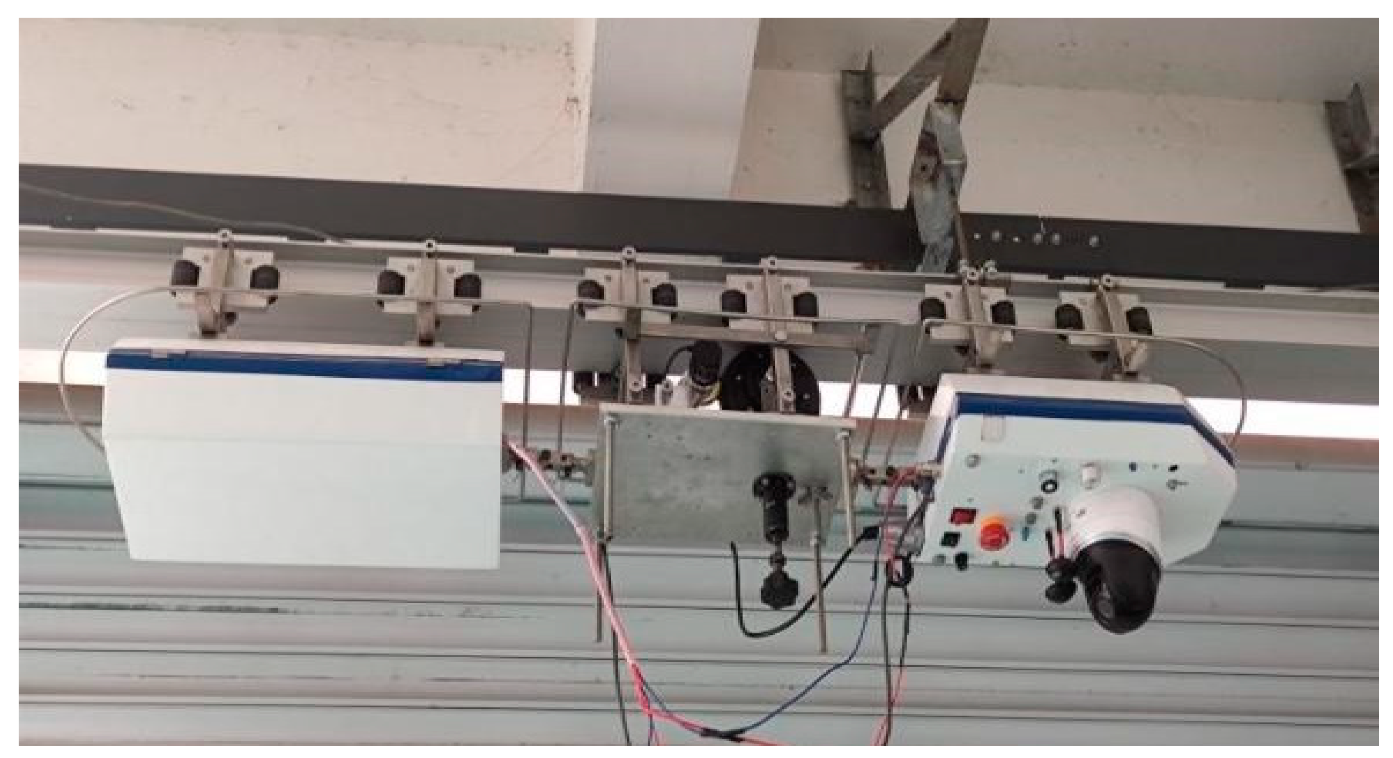
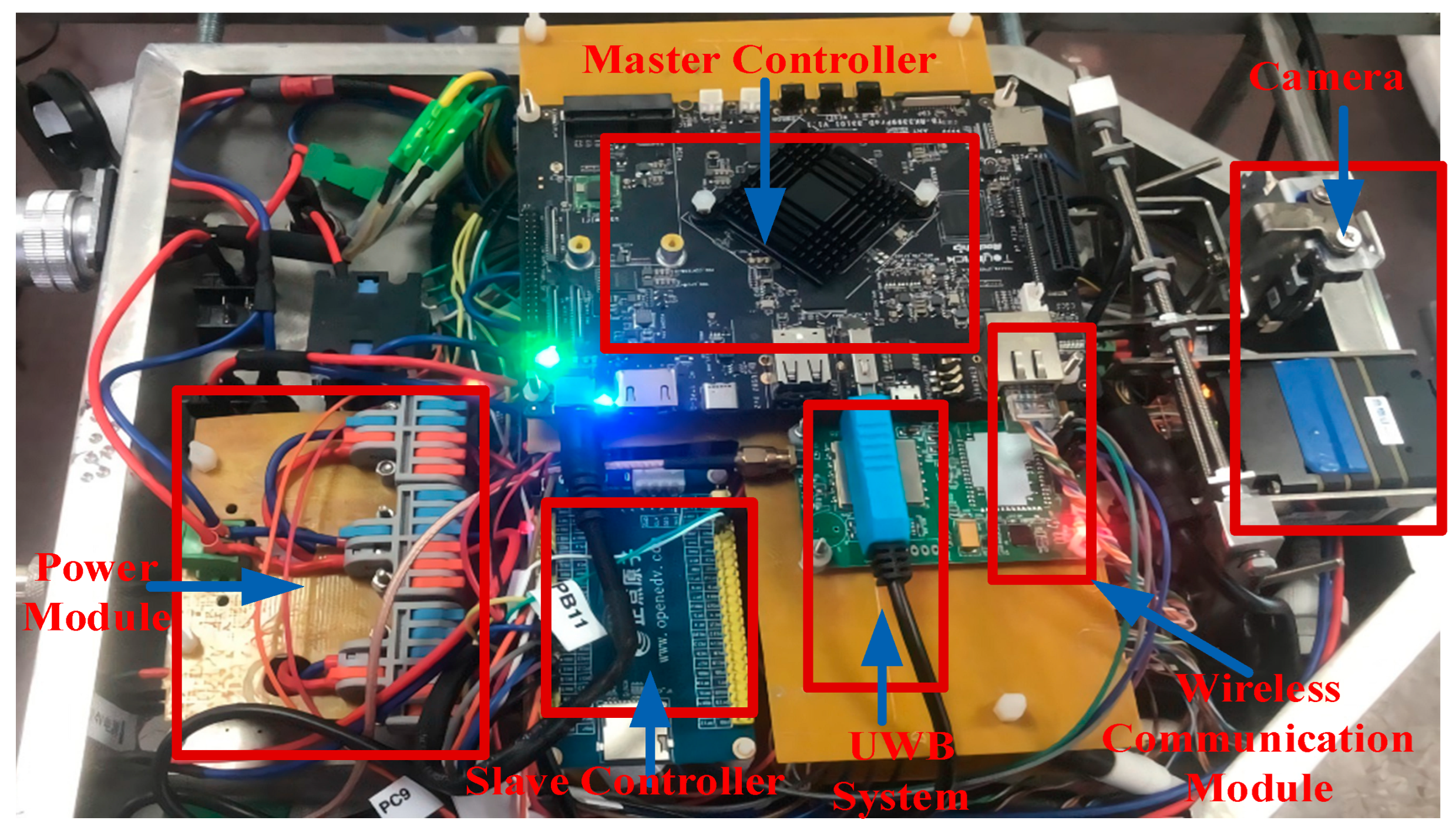
2.2. UWB Positioning

In the UWB positioning part, the signal arrival time difference algorithm (TDOA) is used to complete the distance calculation, and the Chan optimization algorithm is introduced to optimize the location of TDOA positioning.

2.2.1. Chan Algorithm Based on TDOA

The specific ranging and positioning process of TDOA is as follows:

The label node sends a pulse signal at time $t$, and the 3 base stations receive the signal at time $t_1,t_2,t_3$, respectively, with $r_1,r_2,{\mathrm{a}\mathrm{n}\mathrm{d} r}_3$ indicating the distance between the label node and the three base stations. Then, the distance formula is as follows:

$$d_i=\left(t_r^i-t_s\right)\times c$$

(14)

$$d_j=\left(t_r^j-t_s\right)\times c$$

(15)

Let the coordinates of 3 base stations be $\left(x_1,y_1\right),\left(x_2,y_2\right), \mathrm{a}\mathrm{n}\mathrm{d}\left(x_3,y_3\right)$. If the coordinate of the label node is $\left(x,y\right)$, the difference in distance between base station 1 and base station 2 is $r_{21}=r_2-r_1$, and the difference in distance between base station 1 and base station 3 is $r_{31}=r_3-r_1$. Then, the following equation can be listed as:

$$\left\{\begin{array}{c}{r}_{21}=\sqrt{{\left(x_2-x\right)}^2+{\left(y_2-y\right)}^2}-\sqrt{{\left(x_1-x\right)}^2+{\left(y_1-y\right)}^2}\\ r_{31}=\sqrt{{\left(x_3-x\right)}^2+{\left(y_3-y\right)}^2}-\sqrt{{\left(x_1-x\right)}^2+{\left(y_1-y\right)}^2}\end{array}\right.$$

(16)

After the introduction of the Chan optimization algorithm, the distance difference between each base station and the reference base station 1 can be expressed as $r_{i1}$, and then Equation (16) can be simplified as:

$$r_{i1}^2+2r_{i1}{r}_1=K_i-2x_{i1}{x}_1-2y_{i1}{y}_1-K_1$$

(17)

where $K_i=x^2+y^2$, $x_{i1}=x_i-x_1$, $y_{i1}=y_i-y_1$.

Further, Equation (17) can be simplified as Equation (18):

$$\left\{\begin{array}{c}x=p_1+q_1{r}_1\\ y=p_2+q_2{r}_1\end{array}\right.$$

(18)

$$p_1=\frac{y_{21}{r}_{31}^2-y_{31}{r}_{21}^2+y_{31}\left(K_2-K_1\right)-y_{21}\left(K_3-K_1\right)}{2\left(x_{21}{y}_{31}-x_{31}{y}_{21}\right)},q_1=\frac{y_{21}{r}_{31}-y_{31}{r}_{21}}{x_{21}{y}_{31}-x_{31}{y}_{21}}$$

(19)

$$p_2=\frac{x_{21}{r}_{31}^2-x_{31}{r}_{21}^2+x_{31}\left(K_2-K_1\right)-x_{21}\left(K_3-K_1\right)}{2\left(x_{21}{y}_{31}-x_{31}{y}_{21}\right)},q_2=\frac{x_{21}{r}_{31}-x_{31}{r}_{21}}{y_{21}{x}_{31}-y_{31}{x}_{21}}$$

(20)

If Equations (19) and (20) is incorporated into Equation (18), the following is obtained:

$$A{r}^2+B{r}_1+C=0$$

(21)

where $A=q_1^2+q_2^2-1$, $B=-2\left[q_1\left(x_1-p_1\right)+q_2\left(y_1-p_2\right)\right]$.

In sum, two solutions for r can be obtained. One of the solutions can be eliminated based on prior information. The position coordinate $(x,y)$ of the label node can be found by plugging the valid solution into Equation (18).

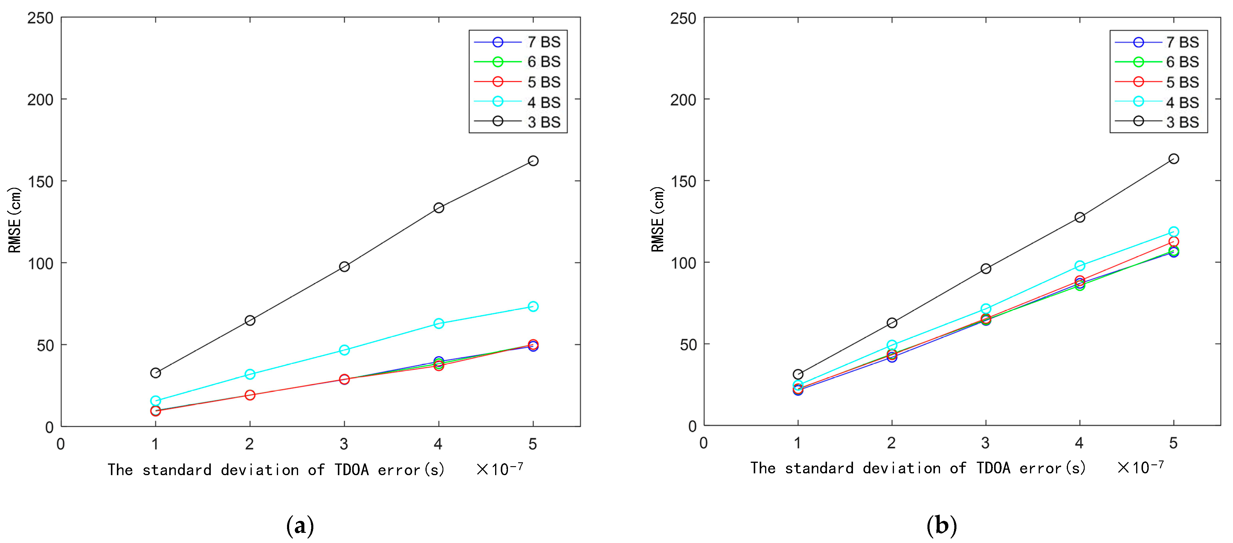
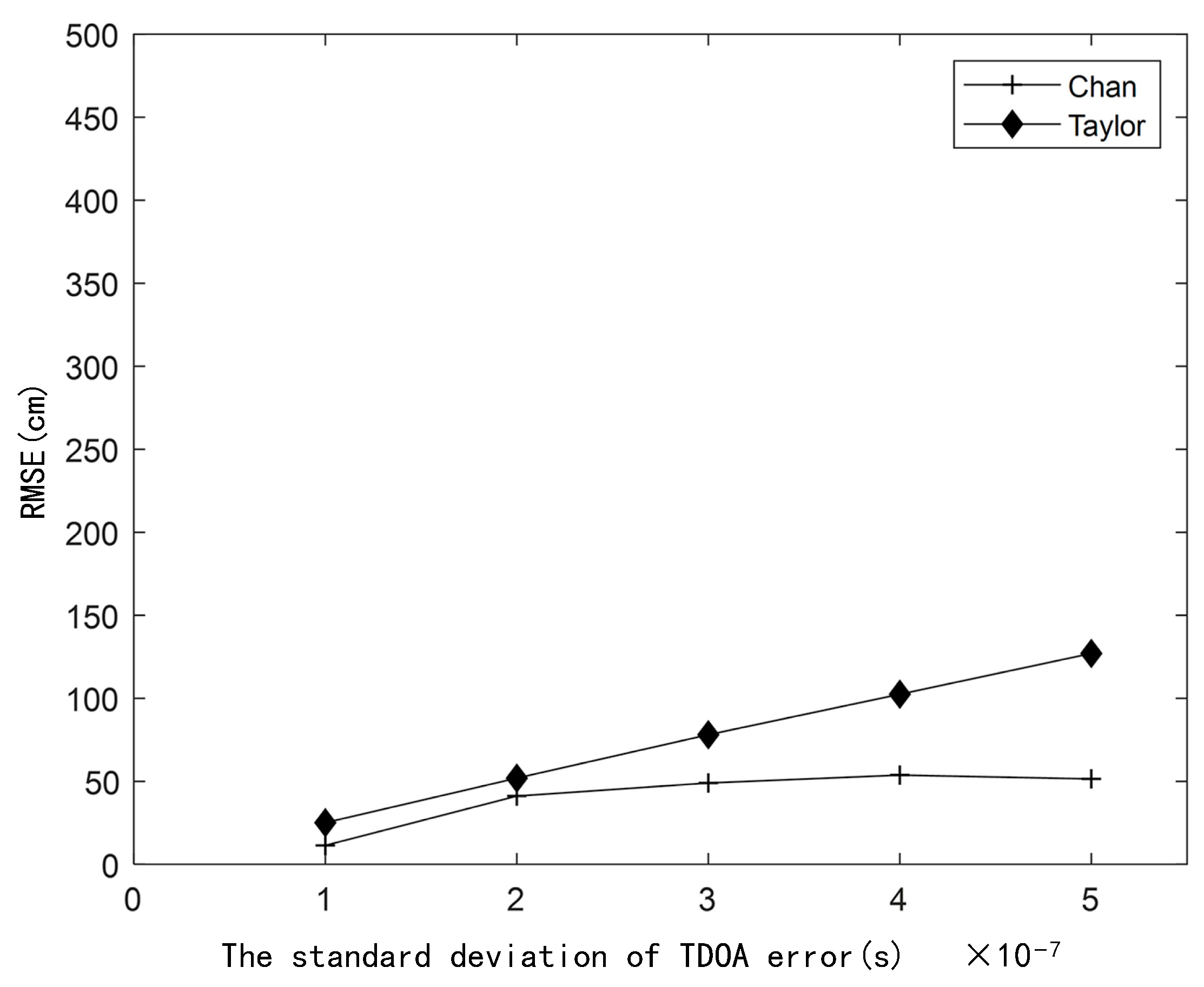
2.2.2. Performance Comparison Experiment between Chan Algorithm and Taylor Algorithm

In the white Gaussian noise environment, the MATLAB2018b simulation is used to verify the impact of different base station numbers and different TDOA errors on the positioning performance of the Chan algorithm and Taylor algorithm. The standard deviations of the TDOA error are 0.1 μs, 0.2 μs, 0.3 μs, 0.4 μs, and 0.5 μs, and the simulation radius is 200 m.

Figure 3 shows that in the Gaussian noise environment, the positioning accuracy of the Chan positioning algorithm increases with an increase in the number of base stations involved in positioning, which is due to the increase in the number of TDOA measurements that can be utilized. However, it can also be seen that when there are more than 5 base stations, the positioning accuracy does not change much, and the positioning performance reaches an optimal level. When the number of base stations is more than 4, the positioning performance of the Taylor algorithm reaches a better level, but it is inferior to that of the Chan algorithm. Therefore, the number of positioning base stations of the rail-mounted robot material distribution system in this paper is selected as 4.

Next, the positioning performance of the Chan algorithm and Taylor algorithm is compared based on 4 base stations. Figure 4 shows the performance comparison of the algorithm with the standard deviation of TDOA error as 0.1 μs, 0.2 μs, 0.3 μs, 0.4 μs, and 0.5 μs; the simulation radius of 200 m; and the mean of 100 positioning errors.

Figure 4 shows that the performance of the Chan algorithm is superior to that of the Taylor algorithm when four base stations are used in the positioning system in the Gaussian noise environment. The Chan algorithm can use all TDOA information to obtain a more accurate solution, so it can adapt to different measurement environments.

3. Results and Discussion

In this section, we introduce the experimental environment and robot configuration. The accuracy of the UWB positioning module is tested. The experiment of the improved Dijkstra algorithm in dynamic programming and conflict coordination is carried out, and its results are compared with the results of the traditional Dijkstra algorithm.

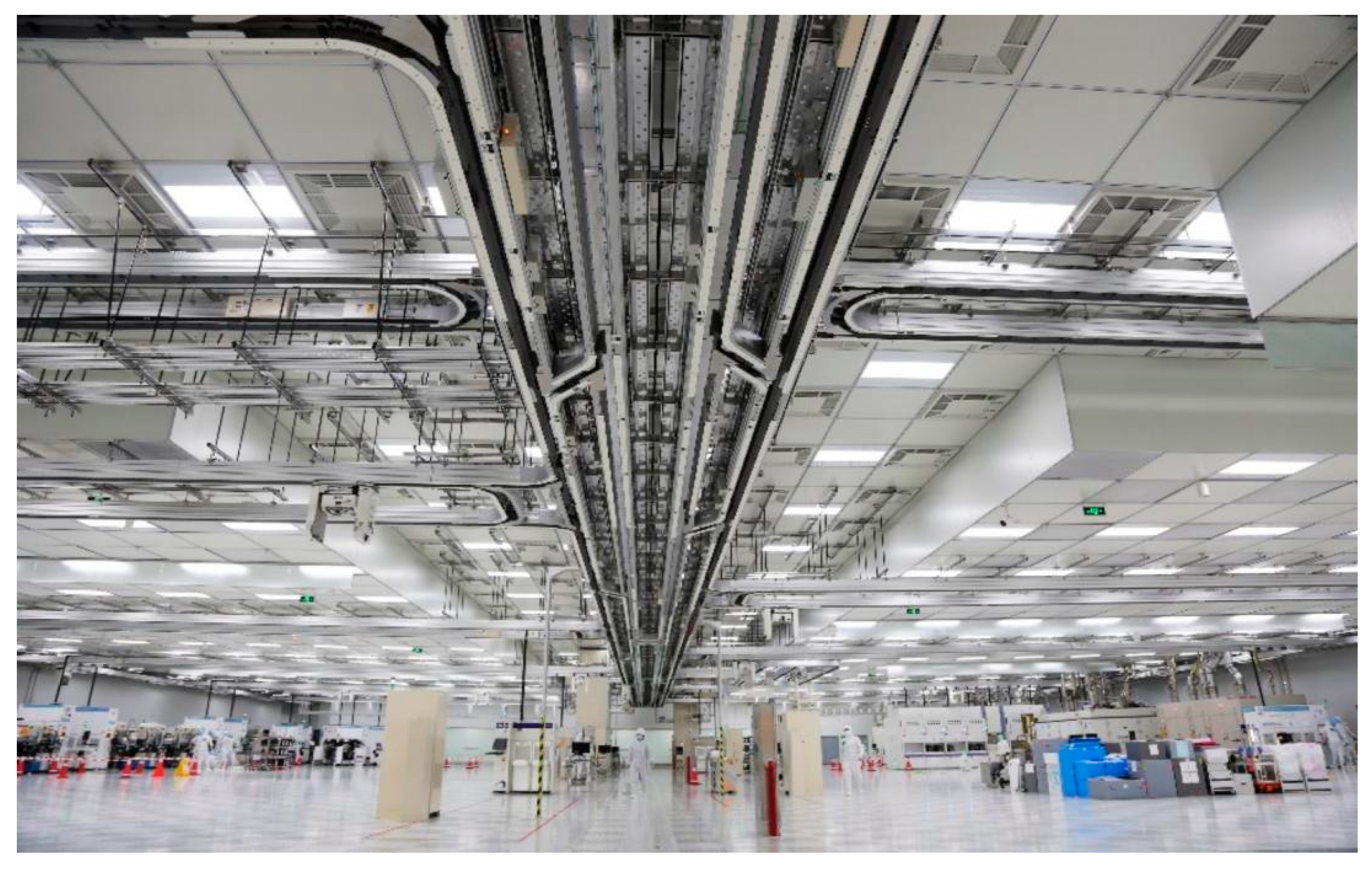
3.1. Experimental Scenarios

The physical object of the rail-mounted logistics robot designed in this paper is shown in Figure 5, which is composed of three parts: material storage bin, power supply bin, and control bin. The control bin of the robot includes a control device, a data acquisition device, a driving device, etc. The internal layout of the robot control bin is shown in Figure 6, which mainly includes the main controller RK3588, the co-controller STM32F1, the power module, the UWB positioning module, etc. Figure 7 shows the application scenario of a rail-mounted logistics robot.

3.2. UWB Positioning Accuracy Test

3.2.1. The Ranging Test

The ranging experiment tested the error of ranging between a label node and a base station node. The test distance range of this test was 200–300 m. After the base station and the label were placed, the real distance was measured and recorded using a laser ruler, and then 20 measured values were obtained using UWB ranging. The average value of one measured value was calculated, and the distance between the base station and the label was changed after a test. A total of 10 groups of tests were completed, and the results are shown in

Table 3. The results of the UWB ranging test.

Serial Number	The Mean Value of the UWB Measurements (m)	Actual Distance (m)	Error (m)
1	206.41	206.27	0.14
2	211.37	211.23	0.13
3	222.12	222.33	0.21
4	231.99	231.80	0.19
5	246.87	246.69	0.18
6	248.52	248.67	0.15
7	261.80	261.62	0.18
8	271.59	271.44	0.15
9	281.71	281.54	0.17
10	284.03	284.13	0.10

.

As calculated from Table 3, the average ranging error is $\pm 0.11$ m. Therefore, the UWB positioning system in this paper can measure stable distance information and provide a reliable data source for the robot’s accurate positioning.

3.2.2. The Positioning Test

The positioning test was conducted in an indoor space with dimensions of 200 m × 200 m. The coordinates of the four base stations were (0, 0), (0, 200), (200, 0), and (200, 200), and the coordinate unit was a meter. Ten known coordinate points were selected in the above space, 50 data points were tested by UWB for each point, and the mean value was obtained. The test results are shown in

Table 4. The results of the UWB positioning test.

Serial Number	The Mean Coordinates of the UWB Measurements (m)	Actual Coordinates (m)	Error (m)
1	(101.22, 101.22)	(101.10, 101.10)	(0.12, 0.12)
2	(100.31, 131.64)	(100.01, 131.48)	(0.03, 0.16)
3	(121.76, 111.51)	(121.59, 111.36)	(0.17, 0.15)
4	(128.70, 128.63)	(128.83, 128.77)	(−0.13, −0.14)
5	(141.89, 171.22)	(141.71, 171.10)	(0.18, 0.12)
6	(151.99, 151.38)	(151.80, 151.25)	(0.19, 0.13)
7	(161.52, 111.61)	(161.02, 111.45)	(0.50, 0.16)
8	(171.75, 181.52)	(171.58, 181.37)	(0.17, 0.15)
9	(190.98, 151.46)	(190.89, 151.32)	(0.09, 0.14)
10	(181.55, 181.75)	(181.40, 181.58)	(0.15, 0.17)

.

From Table 4, it can seen that the positioning errors of the UWB positioning coordinates in the x-axis and y-axis can be calculated as $\pm 0.19$ m and $\pm 0.17$ m, respectively, which meet the requirements of practical applications.

3.3. Dynamic Test Experiment

In order to verify the feasibility of the aforementioned path-planning algorithm, Matlab is used to verify the algorithm combined with an example. Figure 8 shows the simulation diagram of the running environment of the rail-mounted robot. The workshop map layout is created using the raster method. Among them, the white grid represents the track, which is a passable path. The black grid represents the impassable path. The orange grid represents the material station in the workshop. The grid number represents the workstation number. The mode of operation of the robot in orbit is a two-way single lane.

At one time, there were three machines on the track moving to three different target nodes. Figure 9a shows the path initially planned by the traditional Dijkstra algorithm, and Figure 9b shows the path dynamically adjusted by the improved Dijkstra algorithm. In the figures, the three lines with different colors represent the planned paths of the three robots, respectively. A triangle represents the starting point, and a circle represents the ending point. The line colors are blue, red, and green in order of robot priority from highest to lowest. Figure 9c,d show the spatio-temporal graphs of the planned path before and after dynamic adjustment, respectively.

Table 5. Relevant parameters before and after dynamic adjustment.

Robots Serial Number	Priority	Initial Site	Target Site	The Planned Path before the Dynamic Adjustment	The Planned Path after the Dynamic Adjustment
Blue $r_1$	P1	116	231	77-76-206-204-243	77-76-206-204-243
Red $r_2$	P2	168	236	233-27	233-206-204-74-76-27
Green $r_3$	P3	274	102	149-134	149-214-200-135-134

shows relevant parameters before and after dynamic adjustment.

Comparing Figure 9a with Figure 9b, it can be observed that the blue robot with the highest priority during the initial path planning did not change the planned trajectory after the dynamic adjustment, whereas the red robot and the green robot made dynamic adjustments. Since the blue robot traveled according to the established route, its traveling time did not change. Comparing Figure 9c with Figure 9d, it can be observed that in order to prevent an on-orbit collision, the running time of the red robot and green robot increased by 30 s and 40 s, respectively, but the on-orbit collision and congestion problems of the robots are avoided.

3.4. Formatting of Mathematical Components

The following considers the on-orbit collision of two robots as an example to conduct a simulation test and analysis.

Table 6. The relevant parameter settings for the on-orbit operation of the robots.

Robots Serial Number	Priority	Initial Site	Target Site	The Planned Path before the Dynamic Adjustment
$r_5$	P1	222	51	222-141-76-80-51
$r_6$	P2	12	168	12-11-76-168

shows the relevant parameter settings for the on-orbit operation of the robots.

Based on the task parameters listed in Table 6, Figure 10a shows the initial path planned by the distribution system for robots $r_5$ and $r_6$. In Figure 10a, the initially planned paths of robot r₅ and robot r₆ overlap between sections 76-141-168 of the station, resulting in an on-orbit collision between the two robots. Since robot r₅ has a higher priority than robot r₆, the path of the robots needs to be adjusted. The time taken and distance traveled by robot r₆ are calculated to take delay waiting and replanning respectively, and the results are shown in

Table 7. Comparison of different dynamic adjustment strategies.

Adjusting Policies	Path	Travel Time (s)	Distance (m)
Initial planning	12-11-76-168	155.7	140
Delay waiting	12-11-76-168	231.4	140
Replanning	168-143-141-12-13-78	197.1	160

.

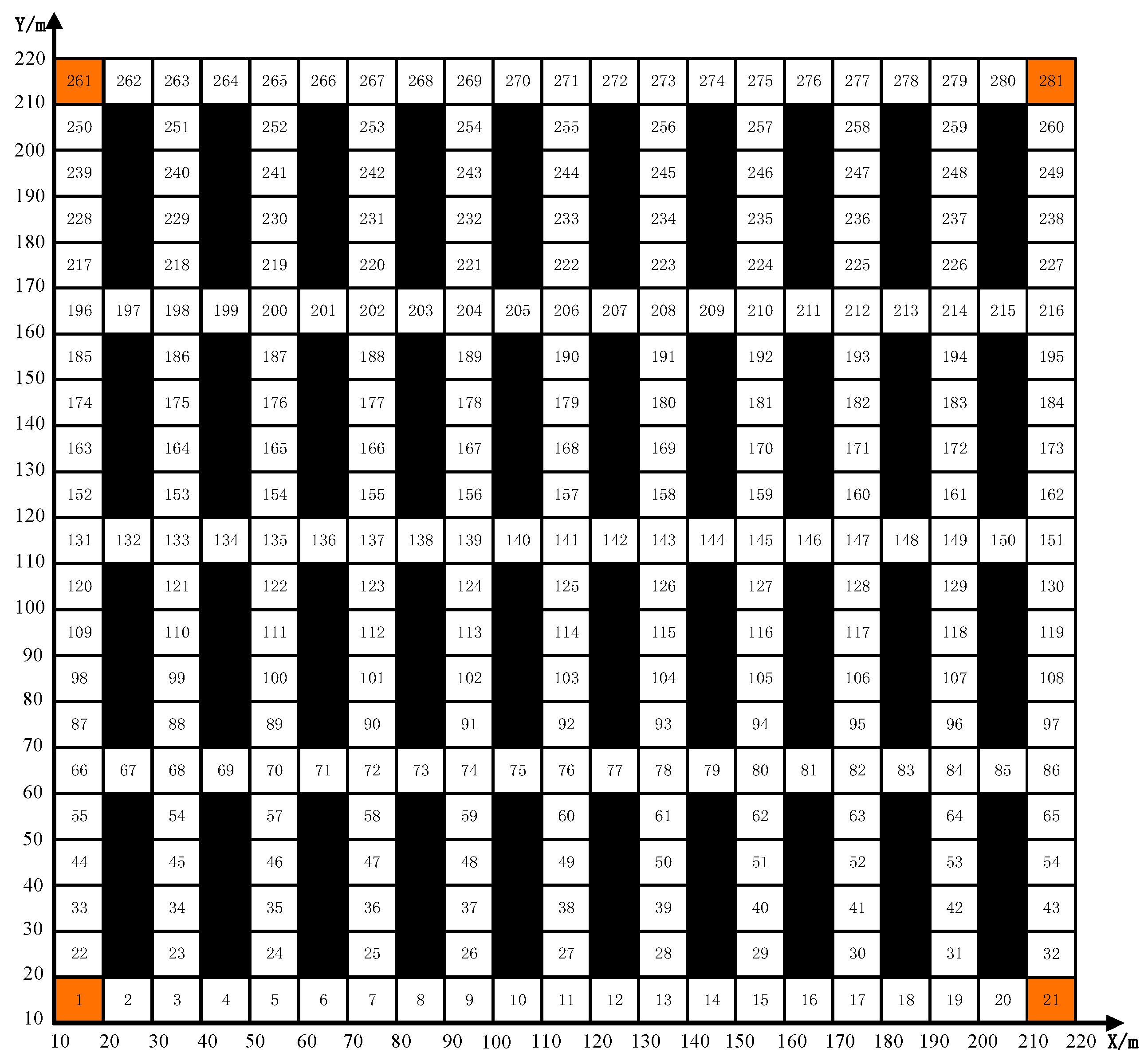
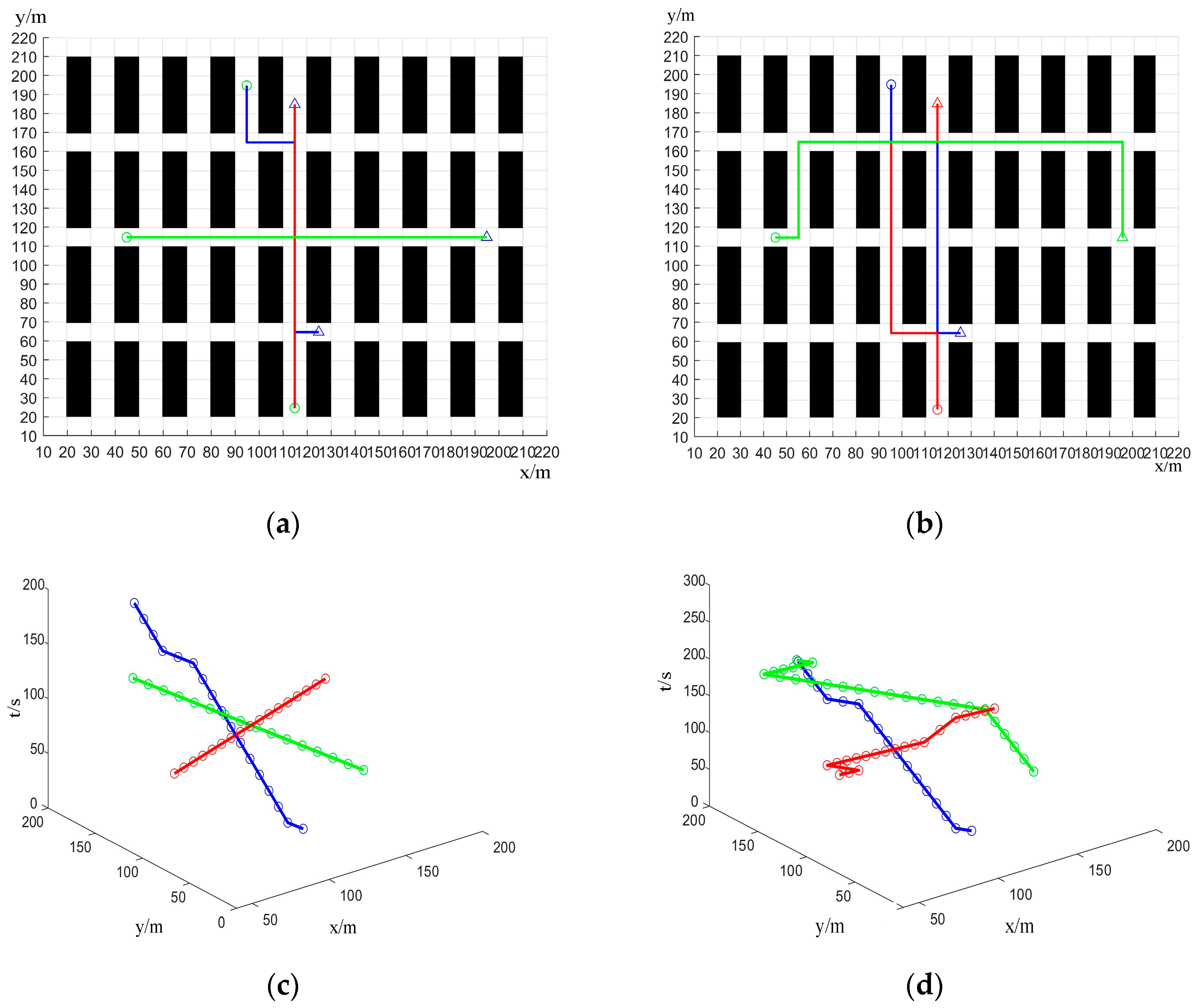
• Delay waiting: As shown in Table 7, if the robot chooses to wait for a delay at station 60 before a conflict occurs, the robot can continue to pass when it passes through station 76. When the delay waiting strategy is adopted, the total traveling time of the robot is 221.4 s, the waiting time is 75.7 s, and the traveling distance remains unchanged. After the robot adopts the delay waiting strategy, the time of executing the distribution task increases by 48.62%, and the driving path does not change.
• Replanning: As shown in Table 7, after the replanning strategy is adopted, the robot’s traveling time is 197.1 s and its traveling distance is 150 m. After replanning, the delivery time and driving distance increase by 25.59% and 14.28%, respectively. Therefore, adopting the replanning strategy to solve the conflict between two robots can improve the efficiency of distribution.

To sum up, in this case, when the robots encounter conflict in opposite directions, the replanning strategy takes 14.28% longer driving distance than the delayed waiting strategy, but the replanning strategy takes 17.82% less time than the delayed waiting strategy. Therefore, the replanning strategy was chosen to improve the efficiency of material distribution. After replanning, the driving paths of the two robots are shown in Figure 10b.

4. Conclusions

This paper presents an enhanced version of the Dijkstra algorithm for the purpose of path planning in rail-hung logistics robots. The proposed algorithm incorporates a real-time node occupancy and time window conflict judgment model to facilitate global path planning and conflict coordination in multi-robot systems. One of the key contributions is the incorporation of real-time node occupancy, which enables the identification of all the shortest feasible routes across various tasks. Additionally, the introduction of a time window conflict judgment model effectively mitigates route conflicts that may arise when executing multiple tasks. This model, in conjunction with system priority setting and conflict coordination strategies, facilitates the achievement of optimal path planning for the system. A Chan algorithm utilizing the Time Difference of Arrival (TDOA) was presented as a means to achieve Ultra-Wideband (UBW) placement, with the objective of accurately locating rail-mounted logistics robots.

Compared with the traditional Dijkstra algorithm, the algorithm proposed herein can not only plan the shortest path when executing multiple tasks but also determine whether the path of each task is in conflict and the type of conflict. According to the priority of the task and the conflict coordination strategy, the task path is either replanned or delayed. The results show that although the travel distance after replanning is 14.28% more than that after delay waiting, the travel time of the former is reduced by 17.82%. Therefore, choosing to replan when encountering path conflicts can improve the efficiency of executing multi-tasks. In the section on the UWB positioning algorithm, we compared the Chan algorithm based on TDOA with the Taylor algorithm based on TDOA. When the number of positioning base stations was four, the performance of the former was significantly better than that of the latter. In the accuracy test, the error in the former was within the allowable range. Therefore, the Chan algorithm based on TDOA was selected, which can provide accurate positioning information for the robot.

Based on the above-mentioned experimental results, our proposed algorithm can plan a conflict-free optimal path and dynamically adjust the on-orbit conflicts in real time to avoid track congestion when multiple robots execute the job.

References

1. Lewis, R.H.; Papadimitriou, H.C. Elements of the Theory of Computation. ACM SIGACT News 1998, 29, 62–78. [Google Scholar] [CrossRef]
2. Cook, S.A. The Complexity of Theorem Proving Procedures. In Proceedings of the 3rd Annual ACM Symposium on Theory of Computing, Shaker Heights, OH, USA, 3–5 May 1971; pp. 151–158. [Google Scholar]
3. Wang, X.; Zhang, H.; Liu, S.; Wang, J.; Wang, Y.; Shangguan, D. Path planning of scenic spots based on improved A* algorithm. Sci. Rep. 2022, 12, 1320. [Google Scholar] [CrossRef] [PubMed]
4. Sang, H.; You, Y.; Sun, X.; Zhou, Y.; Liu, F. The hybrid path planning algorithm based on improved A* and artificial potential field for unmanned surface vehicle formations. Ocean Eng. 2021, 223, 108709. [Google Scholar] [CrossRef]
5. Hartomo, K.; Ismanto, B.; Nugraha, A.; Yulianto, S.; Laksono, B. Searching the shortest route to distribute disaster’s logistical assistance using Dijkstra method. J. Phys. Conf. Ser. 2019, 1402, 077014. [Google Scholar] [CrossRef]
6. Ming, Y.; Li, Y.; Zhang, Z.; Yan, W. A survey of path planning algorithms for autonomous vehicles. Vehicles 2021, 3, 448–468. [Google Scholar] [CrossRef]
7. Baoye, S.; Zidong, W.; Lei, Z. An improved PSO algorithm for smooth path planning of mobile robots using continuous high-degree Bezier curve. Appl. Soft Comput. J. 2021, 100, 106960. [Google Scholar]
8. Hu, Y.; Yang, S.X.; Xu, L.Z.; Meng, M.H. A Knowledge Based Genetic Algorithm for Path Planning in Unstructured Mobile Robot Environments. In Proceedings of the 2004 IEEE International Conference on Robotics and Biomimetics, Shenyang, China, 22–26 August 2004; pp. 767–772. [Google Scholar]
9. Roberge, V.; Tarbouchi, M.; Labonté, G. Comparison of Parallel Genetic Algorithm and Particle Swarm Optimization for Real-Time UAV Path Planning. IEEE Trans. Ind. Inform. 2013, 9, 132–141. [Google Scholar] [CrossRef]
10. Nazarahari, M.; Khanmirza, E.; Doostie, S. Multi-objective multi-robot path planning in continuous environment using an enhanced genetic algorithm. Expert Syst. Appl. 2019, 115, 106–120. [Google Scholar] [CrossRef]
11. Garcia, M.P.; Montiel, O.; Castillo, O.; Sepulveda, R.; Melin, P. Path planning for autonomous mobile robot navigation with ant colony optimization and fuzzy cost function evaluation. Appl. Soft Comput. 2009, 9, 1102–1110. [Google Scholar] [CrossRef]
12. Miao, C.; Chen, G.; Yan, C.; Wu, Y. Path planning optimization of indoor mobile robot based on adaptive ant colony algorithm. Comput. Ind. Eng. 2021, 156, 107230. [Google Scholar] [CrossRef]
13. Sharkawy, A.-N.; Papakonstantinou, C.; Papakostopoulos, V.; Moulianitis, V.C.; Aspragathos, N. Task Location for High Performance Human-Robot Collaboration. J. Intell. Robot. Syst. 2020, 100, 183–202. [Google Scholar] [CrossRef]
14. Dijkstra, E.W. A note on two problems in connexion with graphs. Numer. Math. 1959, 1, 269–271. [Google Scholar] [CrossRef]
15. Zhang, F.B. Three fastest shortest path algorithms on real road networks. J. Geogr. Inf. Decis. Anal. 1997, 1, 69–82. [Google Scholar]
16. Ab Wahab, M.N.; Nefti-Meziani, S.; Atyabi, A. A comparative review on mobile robot path planning: Classical or meta-heuristic methods? Annu. Rev. Control 2020, 20, 50. [Google Scholar] [CrossRef]
17. Sunita; Garg, D. Dynamizing Dijkstra: A solution to dynamic shortest path problem through retroactive priority queue. J. King Saud Univ. Comput. Inf. Sci. 2021, 33, 364–373. [Google Scholar] [CrossRef]
18. Huang, Y.; Sun, J. Research on improved Dijkstra algorithm path planning based on automated wharf. Electron. Des. Eng. 2023, 31, 37–41. [Google Scholar]
19. Qing, G.; Zheng, Z.; Yue, X. Path-Planning of Automated Guided Vehicle Based on Improved Dijkstra algorithm. In Proceedings of the 2017 29th Chinese Control and Decision Conference (CCDC), Chongqing, China, 28–30 May 2017. [Google Scholar]
20. Yulan, Z.; Nannan, H. Airport AGV Path Optimization Model Based on Ant Colony Algorithm to Optimize Dijkstra Algorithm in Urban Systems. Sustain. Comput. Inform. Syst. 2022, 35, 100716. [Google Scholar]
21. Duraklı, Z.; Nabiyev, V. A new approach based on bezier curves to solve path planning problems for mobile robots. J. Comput. Sci. 2021, 58, 101540. [Google Scholar] [CrossRef]
22. Akram, M.; Habib, A.; Alcantud, R.C.J. An optimization study based on Dijkstra algorithm for a network with trapezoidal picture fuzzy numbers. Neural Comput. Appl. 2021, 20, 33. [Google Scholar] [CrossRef]
23. Liu, L.S.; Lin, J.F.; Yao, J.X.; He, D.W.; Zheng, J.S.; Huang, J.; Shi, P. Path Planning for Smart Car Based on Dijkstra Algorithm and Dynamic Window Approach. Wirel. Commun. Mob. Comput. 2021, 2021, 8881684. [Google Scholar] [CrossRef]
24. Szczesniak, I.; Wozna, B. Generic Dijkstra: Correctness and tractability. In Proceedings of the NOMS 2023–2023 IEEE/IFIP Network Operations and Management Symposiu, Miami, FL, USA, 8–12 May 2023; pp. 1–7. [Google Scholar]
25. Reed, J.; Rappaport, T. An overview of the challenges and progress in meeting the E-911requirement for locaation. IEEE Commun. Mag. 1998, 36, 30–37. [Google Scholar] [CrossRef]
26. Smolic-Rocak, N.; Bogdan, S.; Kovacic, Z.; Petrovic, T. Time Windows Based Dynamic Routing in Multi-AGV Systems. IEEE Trans. Autom. Sci. Eng. 2009, 7, 151–155. [Google Scholar] [CrossRef]
Figure 1. Flowchart of improving Dijkstra’s algorithm.
Applsci 13 09955 g001
Figure 2. The driving situation of the robot in different sites. (a) Driving out of the initial site; (b) going straight through a station; (c) turning to pass a station; (d) pulling into the target station; (e) driving straight into V k from V j ; (f) turning into V k from V j .
Applsci 13 09955 g002
Figure 3. Error curves of the Chan algorithm and Taylor algorithm with different numbers of base stations and different TDOA errors. (a) Error curves of the Chan algorithm; (b) error curves of the Taylor algorithm.
Applsci 13 09955 g003
Figure 4. Comparison of error curves between the Chan algorithm and Taylor algorithm in four base stations.
Applsci 13 09955 g004
Figure 5. Test site of the rail-mounted robot.
Applsci 13 09955 g005
Figure 6. Interior layout of the control box.
Applsci 13 09955 g006
Figure 7. Application scenario of a rail-mounted logistics robot.
Applsci 13 09955 g007
Figure 8. Grid diagram of robot operating environment.
Applsci 13 09955 g008
Figure 9. (a) The path initially planned by the traditional Dijkstra algorithm. (b) The path is dynamically adjusted by the improved Dijkstra algorithm. (c) The spatio-temporal graph of the planned path before the dynamic adjustment. (d) The spatio-temporal graph of the planned path after the dynamic adjustment. Three lines with different colors represent the planned paths of the three robots, respectively.
Applsci 13 09955 g009
Figure 10. (a) Robot route planned before the dynamic adjustment. (b) Robot route planned after the dynamic adjustment. The two lines with different colors stand for the planned paths of the two robots, respectively.
Applsci 13 09955 g010