Abstract
To improve the global optimization ability and convergence speed of the swarm intelligence algorithm, we proposed a new swarm intelligence optimization algorithm, namely the Oryctolagus cuniculus algorithm. This includes five mechanisms: the determination of safety zones, the cave escape, the agglomeration of Oryctolagus cuniculi, the maintenance of the Oryctolagus cuniculus king, and the zone competition. Each solution is represented by each Oryctolagus cuniculus’s position (including zone number and specific location number). The grass density and safety index at the location of the Oryctolagus cuniculus represents its fitness value. The determination of safety zones implies that predators such as eagles hunt Oryctolagus cuniculi in dangerous zones, and the zone without predators is considered a safety zone. The cave escape refers to the act of Oryctolagus cuniculi using a connected cave system to flee from a dangerous zone and reach a secure zone, thereby evading potential predators. We select the Oryctolagus cuniculus with higher fitness values as the king of each zone, and the Oryctolagus cuniculi gather towards the Oryctolagus cuniculus king. This mechanism ensures that Oryctolagus cuniculus mainly searches in zones with abundant grass and quickly finds the optimal solution. In the maintenance of the Oryctolagus cuniculus king, we choose the one with higher fitness values as the Oryctolagus cuniculus king. Zone competition is induced by an increase in the number of Oryctolagus cuniculi in zones with abundant grass by ordering the fitness values of each zone, and vice versa. We apply the Oryctolagus cuniculus algorithm to the inversion method of the asteroid spectra reflectance template. The experimental results show that compared with artificial rabbit optimization, this algorithm has a faster rate of convergence and better solution, effectively screens the reflectance template, and improves the Doppler difference velocimetry accuracy. In addition, the application of the Oryctolagus cuniculus algorithm to the knapsack problem also performs effectively.
1. Introduction
With the continuous development of scientific research and engineering practice, optimization problems are becoming an important research field. In many practical applications, solutions that are globally optimal or close to optimal are required. However, traditional optimization algorithms face challenges when solving complex problems, such as high computational complexity and slow convergence speed. Therefore, finding new optimization algorithms becomes crucial.
Swarm intelligence optimization algorithms are a stochastic optimization technique. These algorithms are inspired by social organisms and their collaborative behaviours. The core concept of swarm intelligence algorithms is to simulate the interactions and information exchanges among individuals in a group to achieve global optimization. The advantages of swarm intelligence are mainly in the following aspects: first, it has uncertainty, search based on randomness, easy implementation, and can prevent the algorithm from falling into local optima and exploring a larger search space; second, it has a certain degree of stability and robustness, and strong adaptability; third, it is expandable and adaptive, with individuals adjusting their behaviour according to their own situation and the changes in the surrounding environment, and they can adapt to different problems and environments; furthermore, it is easy to implement and has a relatively simple mathematical model, it does not rely on gradient information, and it does not require in-depth analysis of specific problems. At the same time, swarm intelligence optimization algorithms can continuously utilize their group behaviour for comprehensive search during the optimization process, so they have good searchability and strong parallelism and stability when solving optimization problems.
Most swarm intelligence algorithms are inspired by nature. They can be divided into five categories: evolution-based (E.B.) algorithms, swarm-based (S.B.) algorithms, physics/chemistry-based (P.C.B.) algorithms, human-based (H.B.) algorithms, and others [1].
The evolution-based (E.B.) algorithms simulate the law of natural evolution. They are a randomized search method evolved from the evolutionary law of the biological world and Darwin’s survival of the fittest genetic mechanism. Most algorithms are based on natural selection and species migration, such as the genetic algorithm (GA) [2]. With its appearance, many other evolutionary algorithms have been proposed, including the differential evolution algorithm (DE) [3], evolutionary strategies algorithm (ES) [4], bee queen evolutionary algorithm (QE) [5], and so on.
The inspiration for swarm-based (S.B.) algorithms comes from collective behaviours observed in nature, with the most famous algorithm being particle swarm optimization (PSO) [6]. There are some other algorithms, such as the firefly algorithm (FA) [7], the whale optimization algorithm (WOA) [8], the artificial fish swarm algorithm (AFSA) [9], the artificial bee colony (ABC) [10], the cuckoo search (CS) algorithm [11], the virus colony search (VCS) [12], the Harris hawks optimization (HHO) [13]. Additionally, the artificial rabbit optimization algorithm (ARO) [14] utilizes real rabbits’ foraging and hiding strategies and transitions between the two strategies through energy contraction.
Algorithms based on physics/chemistry are proposed by observing physical or chemical phenomena in nature. Examples include the simulated annealing algorithm (SA) [15], the gravitational search algorithm (GSA) [16], and the artificial chemical reaction optimization algorithm (ACROA) [17]. There are also other algorithms, such as the water cycle algorithm (WCA) [18], the collision-based optimization (CBO) [19], the galaxy-based search algorithm (GbSA) [20], the Henry gas solubility optimization algorithm (HGSO) [21], the charged system search algorithm (CSS) [22], and so on.
Algorithms based on humans are developed by utilizing various characteristics related to humans, such as social, emotional, and cultural aspects. These algorithms include the teaching-learning-based optimization algorithm (TLBO) [23], the social and cultural algorithm (SCA) [24], the focus group (FG) algorithm [25], the poor rich optimization algorithm (PRO) [26], the league championship algorithm (LCA) [27], the student psychology-based optimization (SPBO) [28], the tug of war optimization algorithm (TOW) [29], and the human mind search (HMS) [30]. Of course, some optimization algorithms belong to something other than the above four categories due to different sources of inspiration, such as mathematics, economics, and music. These include the stochastic paint optimization (SPO) [31], the supply-demand-based optimization (SDO) [32], the imperialist competitive algorithm (ICA) [33], the soccer league competition algorithm (SLC) [34], and so on.
In this paper, we propose a new swarm intelligence optimization algorithm: the Oryctolagus cuniculus algorithm (OCA), which is inspired by the group behaviour of Oryctolagus cuniculi. We believe that learning from the behaviour of animals in nature can help us design more innovative and efficient optimization algorithms. By Oryctolagus cuniculi avoiding predators’ killing through caves and looking for the safest and most grass-rich location, OCA can quickly find the global optimal solution in the complex search space.
We propose a new swarm intelligence optimization algorithm, OCA, which is applied to celestial velocimetry navigation. When dealing with complex issues, traditional optimization algorithms face problems such as dimensional disasters, local optima, and slow convergence. At the same time, OCA has better global search and adaptability, and can effectively find global optimal solutions. In the Oryctolagus cuniculus algorithm, the specific location of each Oryctolagus cuniculus is regarded as a solution. We use fitness values to measure the quality of each position. In this paper, the smaller the danger index is, the smaller the error of velocity estimation is, and the better the effect is. Oryctolagus cuniculi dig many connected caves to avoid natural enemies and to find the safest place. By controlling and changing the population size of each zone in the algorithm, the comparison between new and old rabbit kings is updated, improving algorithm efficiency, and providing new ideas and methods for solving complex problems. Compared with the artificial rabbit optimization algorithm (ARO) and the sparrow search algorithm (SSA) [35], the cave Oryctolagus cuniculus algorithm takes the position of each Oryctolagus cuniculus as the measurement standard instead of the energy of each rabbit as the fitness function. The ARO uses bypass foraging and random hiding for population activities, whereas the cave Oryctolagus cuniculus algorithm uses the mechanism of predator killing and cave fleeing. First, it uses a wide range of population behaviour to search, so the Oryctolagus cuniculus algorithm has a strong global search ability. Secondly, the zone competition ensures the processing efficiency of the algorithm. In addition, the setting of the safety zone can have a good ability to reduce the dimension when dealing with multidimensional problems and improve the global ability of the algorithm. The Oryctolagus cuniculus king maintenance mechanism makes the algorithm converge faster. Compared with the SSA, OCA does not easily fall into local optimization, has fewer parameters in the experimental process, and has strong stability, all of which have great research significance.
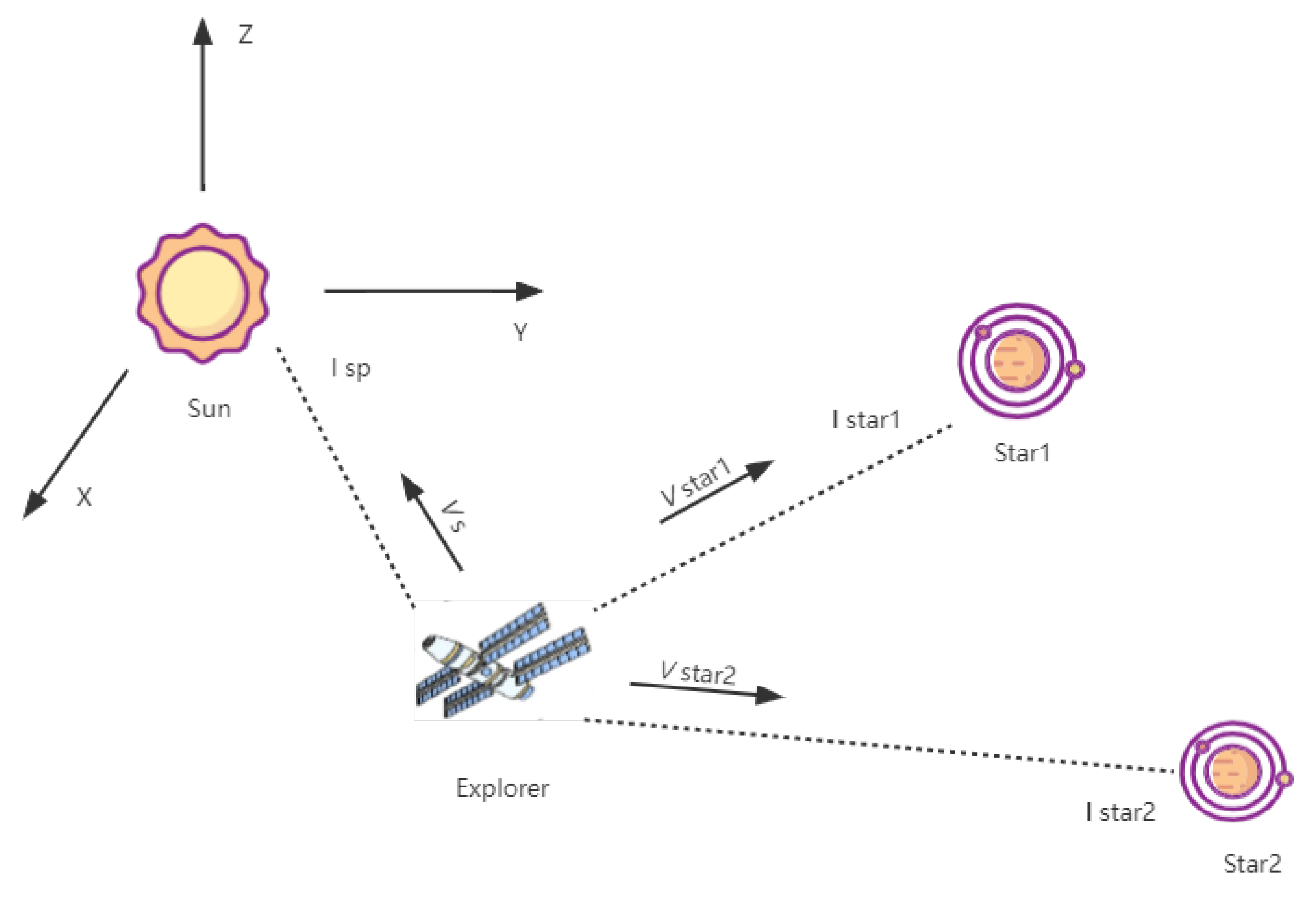
Figure 1 is a schematic diagram of the celestial velocimetry navigation. Deep space exploration technology is an important indicator of a country’s overall national strength and scientific and technological development level. The celestial navigation measurements include the angle measurement, the distance measurement, and the velocity measurement. The angle measurement is the most conventional method of celestial navigation, but its accuracy is limited by the inability to directly provide the bearing information of the target object. The distance measurement, namely X-ray pulsar navigation, has broad prospects in deep space exploration [36,37,38]. The velocity measurement uses a spectrograph to measure the frequency shift of the solar spectrum.

Figure 1.
Diagram of the celestial velocimetry navigation.
The traditional solar Doppler velocimetry navigation does not consider the stability of the solar spectra. It can only provide high-precision positioning and velocimetry information under a stable solar light source. Nevertheless, in practice, the solar spectra are not stable. The reason is that solar activity leads to the distortion of the solar spectra, so we propose a new solar Doppler difference velocimetry navigation. Solar Doppler difference velocimetry navigation can reduce or eliminate the influence of spectral distortion caused by solar activity on velocimetry and improve navigation accuracy. In 2015, in order to resist the velocity deviation caused by solar spectral disturbance, Liu Jin proposed a solar light Doppler difference velocimetry method, which uses the Doppler difference velocity of reflected light from the sun and Mars. This method has a suppressing effect on the common deviation caused by spectral perturbation [39]. However, this celestial Doppler difference measurement method changes the measurement model. Considering factors such as the overlap ratio of the zone of the direct and reflected solar light sources, the diffusion effect of the time difference of light arrival (TDOA), the direction of the solar rotation axis, the differential solar rotation, and the Lambert radiator, Liu Jin established a near-real solar difference deviation model [40,41,42]. However, due to the instability of the astronomical spectra, the spectral velocity estimation method of the ground station has some defects, such as low accuracy and instability, which affect velocimetry navigation.
In order to solve this problem, the velocimetry difference between the solar direct spectrum and the planetary reflectance spectrum is used as the navigation measurement. Because the common deviation is eliminated, the accuracy of the velocity difference measurement is high. The spectra reflectance template inversion method of celestial Doppler difference measurement can reduce the negative impact of the planetary surface absorption effect on velocimetry accuracy. This method uses EMD (empirical mode decomposition) to decompose the measured solar spectra and asteroid spectra, and the corresponding IMFs (intrinsic mode functions) are obtained. The spectra reflectance template inversion method of celestial Doppler difference measurement can reduce the negative impacts of the asteroid surface absorption effect on velocimetry accuracy. This method uses EMD (empirical mode decomposition) to decompose the measured solar and asteroid spectra to obtain the corresponding IMFs (intrinsic mode functions). When selecting reflection templates, it is impossible to traverse each combination because the data are too numerous. Therefore, we manually select favourable reflection templates to provide the initial population for the optimization algorithm in the experiment first, and then use OCA to filter to achieve the best effect, maximize the accuracy of navigation, and test the performance of OCA. We select the appropriate combinations of IMFs through OCA to reflect the astronomical spectra features.
The astronomical spectra are decomposed into multilevel IMFs from low frequency to high frequency, and the IMF is selected with the help of an intelligent swarm intelligence algorithm. EMD can decompose the original signal into multiple signals with different frequencies. These signals are arranged from high frequency to low frequency. The frequency components here are collectively referred to as the IMF. Since the IMF comes from the astronomical spectral profile, the astronomical spectral profile can be characterized by IMF combination, and reflectance templates can be constructed from the spectral profiles of the sun and planets.
We apply OCA to the inversion method of the asteroid spectra reflectance template. Empirical mode decomposition (EMD) processes the astronomical spectra to obtain the IMF that can display the spectral characteristics. OCA screens the IMF, and finally, the combination optimization is realized. The essence of the method is the optimal combination using the intrinsic mode function (IMF). We apply OCA to the inversion of the asteroid spectra reflectance template.
In Section 2, we introduce the biological characteristics of Oryctolagus cuniculus and the algorithm flow. Section 3 introduces the inversion method of asteroid spectra reflectance template for celestial Doppler difference velocimetry. In Section 4, we present the experimental results and analysis. In Section 5, we summarize our work.
2. Oryctolagus Cuniculus Algorithm
To introduce the Oryctolagus cuniculus algorithm, we divide this section into biological characteristics, basic ideas and rules, and algorithm flow. In Section 2.1, we briefly introduce the morphology, distribution, growth and reproduction, habitat, and other properties of Oryctolagus cuniculus. Section 2.2 introduces the concept and main execution rules of OCA. In Section 2.3, we describe in detail the flow and implementation process of the algorithm.
2.1. Biological Characteristics of Oryctolagus Cuniculus
The Oryctolagus cuniculus, also known as the European rabbit, is named for its ability to dig complex cave systems. The complex cave systems are the condition that Oryctolagus cuniculus relies on for survival. The Oryctolagus cuniculus is native to southwest Europe (Spain, Portugal, and western France) and northwest Africa (including Morocco and Algeria). Later, it was widely introduced to other places, often bringing disastrous consequences to local biodiversity [43]. The Oryctolagus cuniculus is one of the smaller mammals, with large and thick ears, shorter ears and hind legs than other rabbit species, thick hind legs, and a short and fluffy tail, with a brown, grey coat, and white lower body, abdomen to tail. The Oryctolagus cuniculus is a social animal. In the biological population, the proportion of female Oryctolagus cuniculi is usually higher than that of male Oryctolagus cuniculi.
The Oryctolagus cuniculus spends most of its active time at dawn and is good at digging caves. Caves are mainly excavated by female Oryctolagus cuniculi during pregnancy. The caves are long and connected. Some caves are used for breeding, and most tunnels may be evacuation sites. The Oryctolagus cuniculus uses its front and rear claws together to dig out the underground passages, forming the system and hiding in caves during the daytime. When encountering danger, the Oryctolagus cuniculus runs to the caves and tries to escape. Oryctolagus cuniculi have strong reproductive abilities, so in places without natural predators, they can proliferate and become a plague. They eat grass and tender branches, but the grass is their main food. They eat up grass, roots, seeds, fruits, and crops, and even destroy trees, leading to land desertification. Oryctolagus cuniculi have many natural enemies. Almost all predators, such as eagles and foxes, prey on Oryctolagus cuniculi. This algorithm simulates the process of various natural enemies hunting Oryctolagus cuniculi.
2.2. Basic Ideas and Rules
In Australia, agriculture and animal husbandry have suffered heavy losses due to the Oryctolagus cuniculus. Oryctolagus cuniculi are naturally fond of drilling caves. They destroy crops and land on farms, causing heavy losses. Therefore, humans began to carry out biological control of the invasive species of Oryctolagus cuniculus. Humans have introduced predators such as foxes and eagles. The predators started to hunt and kill Oryctolagus cuniculi on a large scale in the wild. Humans hope to reduce the number of Oryctolagus cuniculi as much as possible. However, due to the cunning and flexible characteristics of Oryctolagus cuniculi and their ability to escape and flee, making use of their caves, Oryctolagus cuniculi have finally won the “Oryctolagus cuniculus hunting war”.
As social animals, Oryctolagus cuniculi show a certain degree of group wisdom. There are some characteristics of group wisdom of Oryctolagus cuniculi:
- (1)
- Social structure and cooperation: Oryctolagus cuniculi usually live together in social groups composed of multiple individuals. They have shown cooperative behaviour in building and maintaining nests, looking for grass, and protecting themselves. Through cooperation, Oryctolagus cuniculi solve problems together and achieve the group’s overall interests.
- (2)
- Message transmission and warning system: In the Oryctolagus cuniculus community, individuals communicate through voice, posture, and tail swing. When an Oryctolagus cuniculus detects a potential danger or threat, it sends out a specific alarm signal. Other members receive this message and take corresponding actions to start fleeing into the cave to protect the entire population.
- (3)
- Learning and experience transfer: Oryctolagus cuniculi have certain learning abilities and can gain experience by observing the behaviour of other members. For example, an Oryctolagus cuniculus can learn which grasses are safe and which are toxic and then pass the information on to other members. This kind of learning and experience transfer helps the entire population better adapt to the environment and make wiser decisions.
- (4)
- Defence and a rational division of labour: The Oryctolagus cuniculus community shows a high degree of cooperation and a sensible division of labour for the defence of territory and resources. Different individuals play different roles according to their own characteristics and abilities. For example, some Oryctolagus cuniculi are responsible for looking for grass, while others are responsible for looking for safe zones. This division of labour helps to improve the safety and efficiency of the entire population.
To sum up, as social animals, Oryctolagus cuniculi show a certain degree of group wisdom. They show collective wisdom and collaborative behaviour in the face of environmental challenges and survival needs through social structure and cooperation, information transmission and warning systems, learning and experience transmission, and a rational division of labour. These characteristics enable the Oryctolagus cuniculi to adapt more effectively to the environment, to find a safety zone, and improve the survival success rate of the cave population.
We have set some rules for OCA based on the above characteristics. These rules are designed to assist individuals in collaborating within the team, ensuring that individuals do not interfere with each other during task execution or optimization processes, and can limit the search space of algorithms, reduce the number of possible solutions, and improve search efficiency. We achieve overall optimization and problem-solving by clearly defining the behaviour patterns of each individual, ultimately improving the efficiency and results of the entire algorithm. Here are some rules we have established:
- (1)
- In the determination of the mechanism for safety zones, we evaluate the safety index of each zone based on the terrain. Zones with complex terrain and caves are considered safe, whereas open and unobstructed zones are considered unsafe. The survival probability of the Oryctolagus cuniculus is higher in the safety zones.
- (2)
- In the mechanism of the cave escape, Oryctolagus cuniculi seek refuge in zones with caves to avoid being preyed upon. The safest hiding spot in each zone is the deepest cave with rich grass, where the probability of being killed by predators is the lowest. We call the Oryctolagus cuniculus who occupies the safest position the king of the Oryctolagus cuniculus.
- (3)
- In the mechanism of the agglomeration of Oryctolagus cuniculi, apart from the Oryctolagus cuniculi king, there are two options: running towards the direction of the Oryctolagus cuniculus king or exploring other directions within the zone. We need to specify the directions of two choices, so we set a threshold. When the distance between an Oryctolagus cuniculus and the king is less than the threshold, the Oryctolagus cuniculus instinctively moves closer to the king. When the distance exceeds the threshold, the Oryctolagus cuniculi wander within the zone in search of a safety spot.
- (4)
- In the mechanism of the maintenance of the Oryctolagus cuniculus king, we consider that other Oryctolagus cuniculi may find a safer spot than the Oryctolagus cuniculus king’s spot, or that the new king generated after each iteration may have a higher safety index than the old king’s spot. So, in the maintenance of the Oryctolagus cuniculus king mechanism, we continuously compare to ensure that the position of the king is always the spot we know has the highest safety index.
- (5)
- In the maintenance of zone competition, we stipulate that if a zone performs well, it attracts more Oryctolagus cuniculi and the Oryctolagus cuniculi breed, leading to an increase in the number of Oryctolagus cuniculi in the zone. On the contrary, if a zone performs poorly, the Oryctolagus cuniculi in the zone may be preyed upon by predators or flee to other zones, resulting in a decrease in the number of Oryctolagus cuniculi in the zone. However, each zone has a maximum and minimum population capacity, and once the population capacity of the zone reaches a certain threshold, it no longer changes.
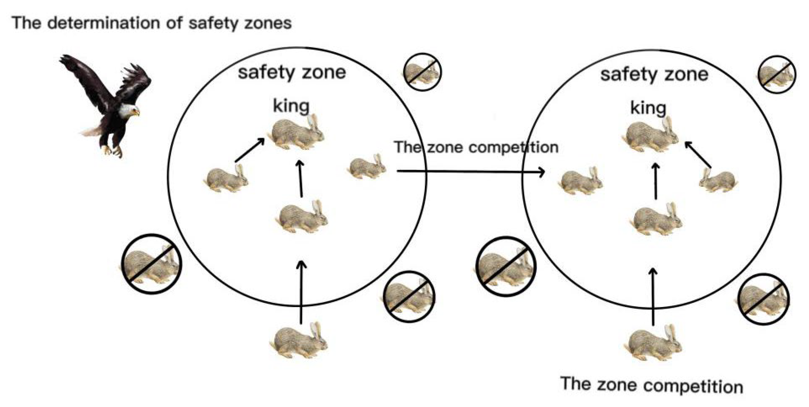
Figure 2 illustrates the movement directions of Oryctolagus cuniculi in different zones. OCA is essentially an operation that continuously updates the positions of each Oryctolagus cuniculus, seeking and exploring better positions to find solutions to the problem. OCA applies the excellent population data from the previous generation to the next generation through selection operations, allowing for faster convergence to the optimal solution. OCA constantly modifies the entire population by eliminating poor positions, aggregating updates, and recombining new positions to prevent the algorithm from getting trapped in local optima. We utilize these variations to steer the algorithm towards better directions, ultimately obtaining the optimal solution to the problem.

Figure 2.
Diagram of Oryctolagus cuniculus algorithm.
In order to achieve global convergence for OCA, it is required that the initial population can reach the global optimal solution within a finite number of steps, and the optimization process should prevent the loss of the already found global optimal solution. The factors related to the convergence of the OCA algorithm mainly include the initial population size, the size and quantity of safety zones, the direction and distance of an Oryctolagus cuniculus’s running, the number of Oryctolagus cuniculi increased and decreased during the zone competition, and the guarantee mechanism of the maintenance of the Oryctolagus cuniculus king. If the initial population is set too small, it does not provide enough sampling points, leading to a decrease in algorithm performance. On the other hand, if the initial population is set too large, although it can increase optimization information and prevent premature convergence, it also results in excessive computational complexity and longer convergence time, thus slowing down the convergence speed. Therefore, when selecting the initial population, an optimal balance needs to be achieved between performance and efficiency.
2.3. Algorithm Flow
OCA includes several intelligent behaviours: the determination of safety zones, the cave escape, the agglomeration of Oryctolagus cuniculi, the maintenance of the Oryctolagus cuniculus king, and zone competition. The general process of OCA is as follows:
In the Oryctolagus cuniculus algorithm, the specific location of each Oryctolagus cuniculus is regarded as a solution. Our goal is to find the safest location. The exact location of each Oryctolagus cuniculus is composed of the zone number and location number. The danger index of the location of each Oryctolagus cuniculus is calculated based on the fitness function. In this paper, the smaller the danger index is, the smaller the error of velocity estimation is, and the better the effect is. In the selection process, the eagle first carries out a large-scale killing of the Oryctolagus cuniculus. The zone where the Oryctolagus cuniculus is killed is an unsafety zone, and the rest is a safety zone. Each safety zone has its own zone number. Oryctolagus cuniculus species dig many connected caves in these safety zones to avoid natural enemies to find the safest place. At first, each safety zone has the same number of Oryctolagus cuniculi. Then, as the zone’s hazard index changes, the population size in each zone also changes accordingly.
In order to improve the efficiency of the algorithm, we first tried to reduce the search range as much as possible. We first divided the entire search zone into several large zones and estimated the safety index of these large zones. If the safety index was small, it indicated that the probability of the optimal result in this large zone was low, and no further search would be conducted in this zone. The remaining large zones were divided into small zones for further search. The reason for not deleting the small zones is that there was a high probability of the optimal result appearing in the small zones at this time. In order to prevent OCA from falling into local optima, we conducted a fine search on the small zones to increase the possibility of finding the optimal solution. We used the maintenance of the Oryctolagus cuniculus king mechanism and zone competition to improve the computational efficiency of the algorithm. The flowchart of the algorithm is shown in Figure 3. Next, we further introduce each mechanism in detail.
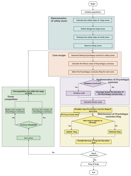
Figure 3.
Flowchart of OCA algorithm.
To illustrate the working process of OCA, we introduce the five main mechanisms of the OCA algorithm in the pursuit and escape behaviour of Oryctolagus cuniculi. In Figure 3, each colour module represents a mechanism. This algorithm mainly includes some mechanisms: the determination of safety zones, the cave escape, the agglomeration of Oryctolagus cuniculi, the maintenance of the Oryctolagus cuniculus king, and zone competition. The first module is the determination of safety zones, which is a mechanism to narrow the search range of algorithms. We remove zones that are unlikely to produce the optimal solution and proceed to the second module, the cave escape. The cave escape is performed to generate Oryctolagus cuniculi in the safety zone determined by the first module. The Oryctolagus cuniculi flee into the cave, and we calculate the fitness value of each Oryctolagus cuniculus to further search for a safe location. Each divided small zone selects an Oryctolagus cuniculus king based on the fitness value, and the Oryctolagus cuniculus king occupies the safest position in each small zone. The third module is the agglomeration of Oryctolagus cuniculi, wherein Oryctolagus cuniculi closer to the Oryctolagus cuniculus king gather towards the Oryctolagus cuniculus king provided by the second module, while Oryctolagus cuniculi farther away from the Oryctolagus cuniculus king swim towards other directions in the zone. The fourth module is the maintenance of the Oryctolagus cuniculus king, which is the optimization mechanism of the entire algorithm, ensuring that the Oryctolagus cuniculus king selected in each zone has the safest zone, and selecting the king of kings based on the fitness value of each zone. The last module is zone competition, wherein zones are sorted based on the fitness value of the Oryctolagus cuniculus king in the previous module. As the number of iterations increases, the number of Oryctolagus cuniculi in each zone is changed based on each zone’s performance to improve the algorithm’s efficiency. As the number of iterations increases, OCA also changes its search method. When the loop completes searching for the best result and reaches the number of iterations, the algorithm is completed.
(Mechanism A) The determination of safety zones: our goal is to determine safety zones. It is almost impossible to achieve optimal values in dangerous zones. Therefore, we search for the optimal value in the safety zone. We first determine the large zone and then the small zone based on the fitness value of each zone. The position of each Oryctolagus cuniculus is determined by both the zone number and the location number. The zone number consists of a large zone number and a small zone number.
Step A1: Determination of large zone: we first divide all search zones into several large zones. Each large zone has its own binary encoding. Then, we estimate the safety index of each large zone to eliminate the more dangerous zones and determine the safety zone for search. The safety index or fitness function for each zone is in Equation (1):
where u = 1,2, …, U is the binary number of digits in the zone number. o = 1,2, …, O is the binary number of digits in the location number. In this mechanism, we set all o to 0 in order to control variables. n is the number of zones selected based on the ranking of the safety index from highest to lowest. represents the entire position information of the n-th zone. F represents the fitness function of the algorithm. represents the fitness function of the n-th zone.
Step A2: Determination of small zone: we further screen the selected large zones and divide large zones into small zones. Divide the large zone into 2U small zones. The more digits, the more detailed the position information and the smaller the scope. Determine the appropriate U based on the fitness function. Our main task in this step is to extend the zone number from the first position to the u position. In this way, the complete position information of each Oryctolagus cuniculus can be represented as in Equation (2):
where n = 1,2, …, N represents the number of the zone, and w = 1,2, …, W represents the number of Oryctolagus cuniculi in the zone, represents the w-th Oryctolagus cuniculus in the n-th zone of the complete position information, Y represents the zone number, and Z represents the location number. Due to the lack of Oryctolagus cuniculus location information when the determination of safety zones is occurring, the part of the location number is uniformly set to 0.
(Mechanism B) The cave escape: after determining the zone number of each zone, we generate fleeing Oryctolagus cuniculi for each zone and begin a large-scale search in each safety zone. Each Oryctolagus cuniculus has detailed location information and escapes in the cave of the zone. After the escape, we calculate the fitness value of each Oryctolagus cuniculus and label the Oryctolagus cuniculus with the best fitness value in each zone as the Oryctolagus cuniculus king.
Step B1: The generation of Oryctolagus cuniculi: after determining the zone number for each zone, generate a certain number of Oryctolagus cuniculi. Generate detailed location information for each Oryctolagus cuniculus bit according to Equation (3):
where Ps is a parameter to adjust the dispersion of Oryctolagus cuniculi running. The larger Ps is, the more scattered the position is, and the smaller Ps is, the less scattered the position is. is the position information of the o-th position of each Oryctolagus cuniculus location number.
Step B2: The calculation safety index: the position information consists of the zone number and location number. The safety index of each zone is represented by the survival of the Oryctolagus cuniculus with the best fitness value; namely, Equation (4):
where Sn is the best safety index for each zone, and represents the complete position information of the best Oryctolagus cuniculus in the n-th zone.
Equation (5) is the position information of the king.
where is the king’s zone number information and is the king’s location number information.
Step B3: The start of the fleeing: after determining the zone number, in each designated safety zone, the same number of Oryctolagus cuniculus cave communities begin to flee. The location number of each Oryctolagus cuniculus cave is randomly updated, and the fitness value is calculated. We register the fitness values of each Oryctolagus cuniculus and proceed to the next step.
Step B4: The choosing of the king: with the specific location of each Oryctolagus cuniculus, we calculate all the Oryctolagus cuniculi in each zone and select the best Oryctolagus cuniculus in each zone through a fitness function, who is labelled as the Oryctolagus cuniculus king. Equation (6) is our normalization process:
where represents the normalized result, represents the fitness value, represents the maximum fitness value found, and represents the found fitness value.
(Mechanism C) The agglomeration of Oryctolagus cuniculus: due to the high probability of the existence of an optimal solution near the king, it is easier to search for the optimal solution by aggregating towards the king. Therefore, we change the position values of the Oryctolagus cuniculi, with some aggregating towards the king and others searching for better solutions. It is a further search of the algorithm.
Step C1: The calculation of distance: calculate the distance between each Oryctolagus cuniculus and the Oryctolagus cuniculus king and compare it with the threshold. In Equation (7), the calculated Hamming distance is expressed as:
where represents modulo two additions, Hd is the distance between the current Oryctolagus cuniculus and king. represents the location information of this current Oryctolagus cuniculus, represents the location information of the king. o is the number of bits of location information.
Step C2: The determination of direction: determine whether each Oryctolagus cuniculus gathers in the direction of the Oryctolagus cuniculus king or runs in other directions based on the threshold τ. Equation (8) represents the change in each bit of Oryctolagus cuniculus information.
where τ is the threshold for determining direction. When is less than or equal to τ, the Oryctolagus cuniculi within the range move towards the king with probability . When is greater than τ, the Oryctolagus cuniculi outside the range continue to explore in other directions with probability . is the position information of the o-th position of each Oryctolagus cuniculus location number.
(Mechanism D) The maintenance of the Oryctolagus cuniculus king: this mechanism is the optimization mechanism in the algorithm. We compare the new and old kings to select the better one, which continuously compares and ultimately saves the optimal solution. The purpose is to accelerate the convergence speed of the algorithm.
Step D1: King showdown: at each iteration, the new Oryctolagus cuniculus king’s position is compared with the old Oryctolagus cuniculus king’s position. In Equation (9):
where is the quality of each Oryctolagus cuniculus king, is the fitness function of this Oryctolagus cuniculus and is the distance between this Oryctolagus cuniculus and current kings. β1 and β2 represent the proportion of these two items in the king showdown, respectively.
Step D2: King update: if the new Oryctolagus cuniculus king’s position is safe, the Oryctolagus cuniculus king is updated. If the position of the old Oryctolagus cuniculus king is even higher, it maintains the role of Oryctolagus cuniculus king. When selecting the Oryctolagus cuniculus king, first select the smallest fitness function for each zone as the Oryctolagus cuniculus king, and document all information of the Oryctolagus cuniculus king:
where is the best information, including the fitness function and location information of the Oryctolagus cuniculus.
(Mechanism E) Zone competition: each zone competes for Oryctolagus cuniculus resources based on the fitness value of each zone. The better-performing zone increases the population of Oryctolagus cuniculi, while the worse-performing zone reduces the number of Oryctolagus cuniculi. Each iteration ranks all zones based on fitness values to evaluate their performance. When the population in each zone increases or decreases to a certain number, the number of Oryctolagus cuniculi does not change. The competition between zones can flexibly change the population size of each zone. By changing the number of Oryctolagus cuniculi, computing resources can be reasonably allocated, improving the computational efficiency of the algorithm, and accelerating its convergence speed.
Step E1: Zone sort: we sort zones according to their fitness values.
Step E2: Quantity adjustment: the zone controls the number of Oryctolagus cuniculi in each zone based on their performance in this iteration. At the beginning, each population has Q Oryctolagus cuniculi, and in each iteration, it increases φ per advantaged zone and decreases η per poor zone. The population change in each zone is shown in Equation (11):
where γ represents the current population size in each zone, and σ is the threshold of names used to distinguish between advantaged and marginalized zones.
Step E3: Limitation of quantity: the zone competition effectively utilizes computing resources and accelerates search efficiency. When the number of advantaged zones increases to ρ, the size of the population in the zone does not increase, and when the number of marginalized zones decreases to δ, the size of the population in the zone is not reduced:
where α represents the number of individuals when they have reached their maximum and minimum capacities. ρ and δ represent the maximum and minimum population numbers, respectively.
Through iteration, the algorithm continuously searches for individual and globally optimal solutions while updating the number and walking direction of the Oryctolagus cuniculus population based on this information. Through iterative optimization, the algorithm continuously searches for the optimal solution and ends the calculation when the stopping condition is met, or the maximum number of iterations is reached.
3. Inversion Method of Asteroid Spectra Reflectance Template
The inversion method of the spectra reflectance template for celestial Doppler difference velocimetry uses EMD (empirical mode decomposition) to decompose the measured astronomical spectra, and the IMF obtained can be used to invert the measured reflectance template. The swarm intelligence algorithm is used to obtain the optimal combination of IMFs. The process is as follows:
- (1)
- Referential velocity difference
The difference between the HE-SRV(HARPS ESO-Solar Radial Velocity) and the HE-ARV (HARPS ESO-Asteroid Radial Velocity) is the HE-SARDV(HARPS ESO-Solar and Asteroid Radial Difference Velocity) , whose expression is given as in Equation (13):
where, i = 0,1,2,3, …, I − 1 is the serial number of the asteroid spectra, and I is the number of the asteroid spectra used.
Since that asteroid is far from the earth, taking the earth as the observer, the motion of the asteroid approximates to a uniform linear motion in a short time. Assume that the OT (observation time) of the i-th asteroid spectra is . The relationship between the difference of OT and conforms to the Equation (14) model:
where a is the real value of acceleration, and ωi is the velocimetry noise of the i-th asteroid spectra. is the difference in velocimetry noise of the asteroid spectra. From the Doppler difference velocimetry model [36], the Doppler difference velocimetry eliminates the Doppler velocity bias at the cost of the slight enlargement of the measurement noise, further improving navigation accuracy. Therefore, Doppler difference velocimetry can improve the navigation performance of autonomous navigation for integrated navigation.
In order to improve the accuracy of the referential velocity difference, the least square method is used to fit OT and the velocity difference. The expression is shown as in Equation (15):
where is the referential velocity difference of the zeroth asteroid spectra and is the referential acceleration.
and a can be solved through Equation (15). Using them, we get the referential velocity difference of the i-th asteroid spectra in Equation (16):
Due to the noise reduction capability of the least square method, the error of is times that of .
- (2)
- EMD
The measured solar spectra and the measured asteroid spectra are decomposed by EMD to obtain the IMFs and their residuals. Assume that and are the residuals of the measured solar spectra and the measured asteroid spectra, respectively.
and (m = 1,2,3, …, M) are the IMFs of the measured solar spectra and the measured asteroid spectra, respectively, where i and I are the same as defined in . m is the number of levels of the IMFs, and M is the maximal number of levels.
- (3)
- Selection of the IMFs
Assume that the chromosome of the individual is X, and the gene on the chromosome is transformed into binary code, as in Equation (17):
where is corresponding to the IMFs of the measured solar spectra, and is corresponding to the IMFs of the measured asteroid spectra. If j is equal to other values, it is meaningless. If xj is equal to 0, the corresponding IMF is not selected; conversely, the corresponding IMF is selected.
- (4)
- Construction of the reflectance template
The reflectance template is the ratio of the solar envelope to the envelope of the i-th asteroid spectra, where the solar envelope is the sum of some IMFs of the measured solar spectra and its residual, and the envelope of the i-th asteroid spectra is that of the i-th measured asteroid spectra. Since xj is equal to 1 or 0, the selection of some IMFs is realized to form the reflectance template. The expression for the reflectance template is given as in Equation (18):
- (5)
- Construction of the virtual asteroid spectra
The reflectance template is applied to the measured solar spectra to obtain the virtual asteroid spectra , where is the element-wise product.
- (6)
- Estimation of the velocity difference by the Taylor method
Assume that the wavelength range of both the virtual asteroid spectra and the measured asteroid spectra are . We take the logarithm of the wavelength and make the non-uniform discrete Fourier transform for the two spectra. The Fourier amplitudes of and are and , and the Fourier phases are and , respectively. In the Taylor method [44], we use two-level searching method to find . This method not only ensures the same searching accuracy and searching range, but also reduces the amount of calculation by a hundredfold.
where is the phase difference between the virtual asteroid spectra and the measured asteroid spectra . k = 0,1, …, K − 1 is the frequency and K is the number of sampling points.
We convert the phase difference into the estimated velocity difference according to Equation (20):
where e is the base of the natural logarithm, , c is the speed of light.
- (7)
- Estimation value of the fitness
We calculate the error between the estimated velocity difference and the referential one through Equation (21):
where is the error between the i-th estimated velocity difference and the referential one of the asteroid, and are the i-th estimated velocity difference and the i-th referential one of the asteroid, respectively. The expression for the fitness function is shown in Equation (22):
where is the mean of errors between the estimated velocity difference and the referential one.
The optimization objective is to minimize the value of the fitness function , and the OCA method is employed to obtain the optimal combination of IMFs.
4. Experimental Results and Analysis
In order to test the performance of OCA, we take the accuracy of the Doppler difference velocimetry between the solar spectra and Ceres spectra as the optimization goal. The paper undertakes the following tasks:
- (1)
- We manually select the most suitable reflection template to provide the initial population for the swarm intelligence algorithms.
- (2)
- We use OCA applied in the inversion method of the asteroid spectra reflectance template.
- (3)
- We investigate the zone competition mechanisms using OCA.
- (4)
- We compare OCA with OCA, GA, SSA, and ARO.
- (5)
- We extend the application of OCA for the 0-1 knapsack problem and compare it with GA, PSO, SSA, ARO, and OCA.
4.1. Experimental Conditions
The spectra used in the experiment come from the European Southern Observatory. ESO is the European Organisation for Astronomical Research in the Southern Hemisphere. It operates the La Silla Paranal Observatory in Chile and has its headquarters in Garching, near Munich, Germany. The measurement instrument is Harps, and the telescope is ESO-3.6. The category and the observation time of the used spectra are shown in Table 1, and other experimental conditions are shown in Table 2.

Table 1.
The category and the observation time of the spectra.
Table 2.
Experimental conditions.
We have listed some variables used in the OCA algorithm and the values set for the variables in Table 2. We explain the settings of these variables as follows:
- The number of digits in the zone number (u): This parameter represents the zone number. We use the first eight bits of binary encoding to divide large and small zones and distinguish different zones.
- The number of digits in the location number (o): This parameter represents the location number. We use the last 10 bits of binary encoding to determine the specific location of the Oryctolagus cuniculus in the zone. This can easily change the individual’s position.
- The number of safety zones (n): We set the number of 20 safety zones. This number can avoid the traps of the algorithm with regard to computation and local optima.
- The initial population in a zone (Q): We set the initial population of each zone to 35 Oryctolagus cuniculi to ensure the ability and diversity to explore the solution space.
- The maximum number of the population that can be accommodated in a zone (ρ): The maximum population in the zone is set to 70 Oryctolagus cuniculi. We set the maximum population size in the zone to avoid excessive consumption of computing resources.
- The minimum number of the population that can be accommodated in a zone (δ): The minimum population in the zone is set to five Oryctolagus cuniculi to ensure the algorithm’s exploration of the zone.
- The number of increased Oryctolagus cuniculi per zone (φ): If the zone performs well, it increases by seven Oryctolagus cuniculi in the next iteration, and it reaches its maximum capacity after increasing by five times.
- The number of reduced Oryctolagus cuniculi per zone (η): If the zone performs badly, it reduces by five Oryctolagus cuniculi in the next iteration, and it reaches its minimum capacity after being reduced by six times.
- The probability of Oryctolagus cuniculi escaping (ps): In the initial search phase, the Oryctolagus cuniculus runs randomly, and the escape probability is set to 0.5.
- The proportion of the fitness value in the king competition (β1) and the proportion of the distance between two Oryctolagus cuniculi in the king competition (β2): A weight of 0.6 indicates the importance of the fitness value in competition, while a weight of 0.4 indicates the importance of the distance in competition, which is a relatively high β value, meaning that the value has a greater impact on competition.
- The threshold for determining direction (τ): We set the threshold for determining the direction to four, which is used to control the running direction of the Oryctolagus cuniculi and plan the different running directions of the Oryctolagus cuniculi, making the algorithm more efficient.
- The probability of changing towards the king (pk): Each bit in the location information has a 0.8 probability of becoming the same as the king, and a certain probability of changing to the king indicates running towards the king.
- The probability of moving in other directions (pd): We set the probability to 0.5 because the Oryctolagus cuniculi need to randomly explore other places.
4.2. Manual Selection for Spectra Reflectance Template
The manual selection of spectra reflectance template inversion is selecting an effective IMF combination to provide the initial population for OCA, which can accelerate the convergence speed of OCA. The reflectance curve is the ratio of the Ceres envelope to the solar envelope. The Ceres envelope is the sum of some IMFs and Ceres residual spectra, while the solar envelope is the envelope of the solar spectra. The expression of the reflectance curve is shown in Equation (23).
where k1 = 1,2, …, M and k2 = 1,2, …, M are the initial number of levels selected of the solar IMFs and the IMFs of Ceres, respectively.
The velocimetry errors of the manual selection of spectra reflectance template inversion for Ceres are shown in Table 3. The maximal error in Table 3 is 5776 m/s, and the minimal one is 1.24 m/s. With a significant difference between them, we can see that it is crucial to select the reflectance template. The effective reflectance curve is applied for the measured solar spectrum, which can effectively reduce the influence of reflectivity on the asteroid; otherwise, the velocimetry is seriously abnormal. Taking the referential velocity difference as the baseline, the error of the velocimetry, by the traditional Taylor method, is 2.85 m/s, and the errors in bold type in Table 3 are lower than that. We can see that the levels of effective combinations of IMFs are concentrated in levels 7~9 of the asteroid spectrum and levels 4~9 of the solar spectrum. Among them, k1 = 4, k2 = 7 is the best combination of IMFs.
Table 3.
Velocimetry errors of the manual selection.
The measurement accuracy of OCA using the manually selected population is significantly higher than that of the random initial population, and its convergence speed is much faster than that of the random initial population. This shows that the effective combination of manually selected IMFs as the initial group can accelerate the convergence speed and improve the measurement accuracy. The favourable template selected manually has a positive impact on improving the accuracy of the celestial Doppler difference velocimetry. In Section 4.4, we use several swarm intelligence algorithms to search IMF combinations to build reflectance templates. We apply them to celestial Doppler difference velocimetry and compare the error and convergence of these algorithms.
4.3. Zone Competition
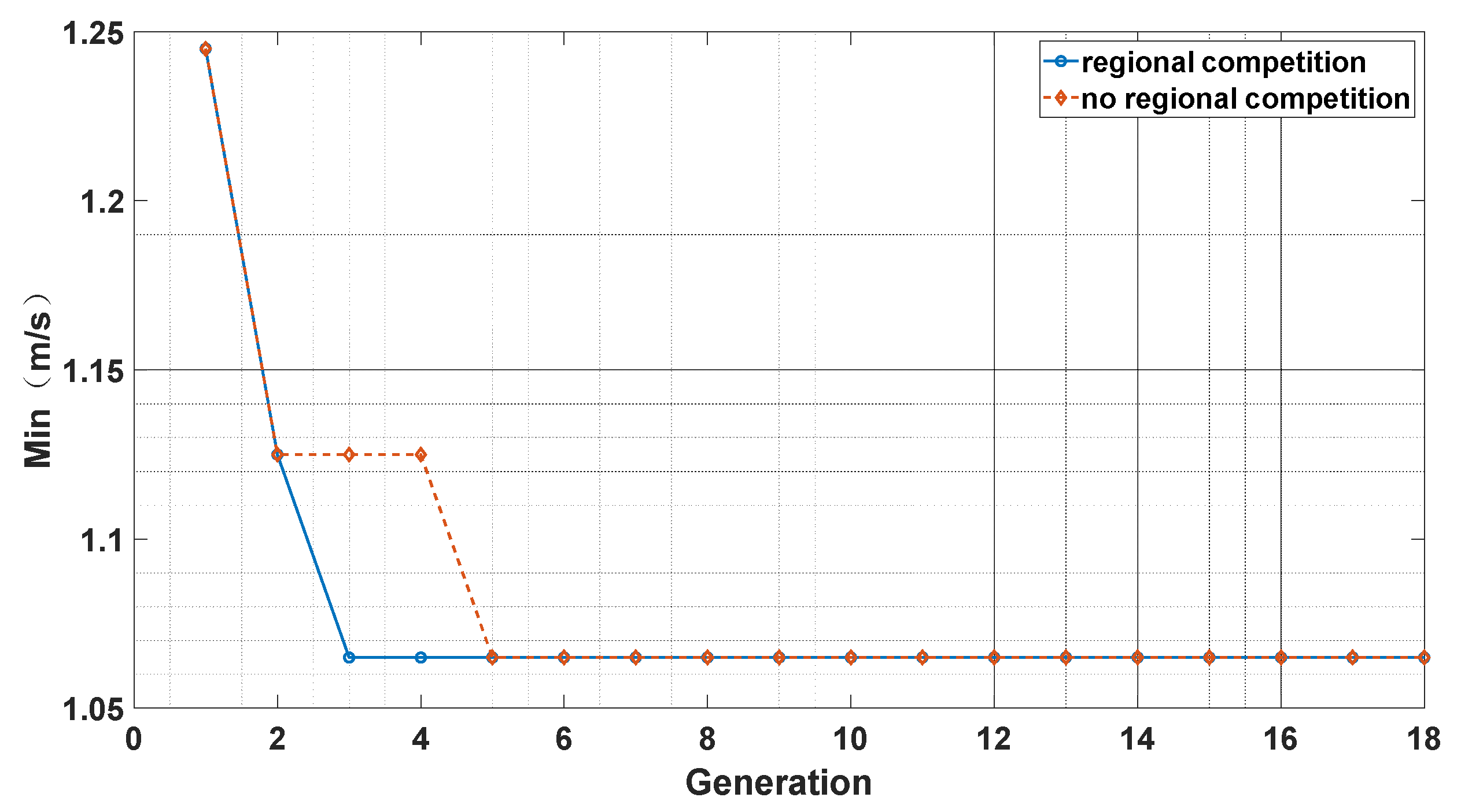
We took the accuracy of the Doppler velocimetry difference between the solar spectrum and the Ceres spectrum as the optimization goal. We compare OCA with a zone competition mechanism to OCA without a zone competition mechanism in Figure 4. We can see that the OCA algorithm with zone competition has a faster convergence speed than the OCA algorithm without a zone competition mechanism. The zone competition mechanism can increase the population density of Oryctolagus cuniculi in safety zones while decreasing the population density of Oryctolagus cuniculi in dangerous zones. This can enhance the efficiency of the algorithm in searching for sub-optimal solutions. Namely, the zone competition mechanism can improve the algorithm’s efficiency and make effective and rational use of resources. The zone competition mechanism also sets maximum and minimum values for the population size in each zone, which helps the algorithm mitigate the risk of falling into a local optimum.
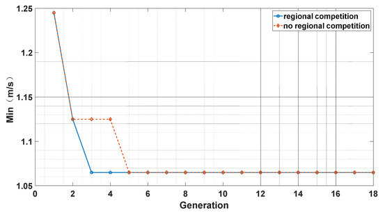
Figure 4.
Comparison of OCA with zone competition and without zone competition.
4.4. Comparisons between OCA and GA, SSA, ARO
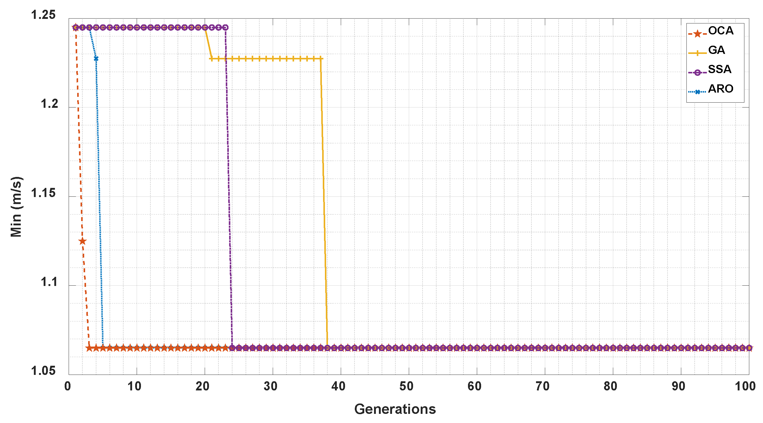
In order to test the performance of OCA, we now compare OCA with GA, SSA, and ARO. We use the sub-optimal combination of IMFs obtained by OCA and other algorithms to construct the reflectance templates for velocimetry. The convergence curve of each algorithm is shown in Figure 5. The x-axis represents the convergence iterations of swarm intelligence algorithms, while the y-axis represents the minimum error achieved by each algorithm.

Figure 5.
Comparison of convergence curves for OCA, GA, SSA, ARO.
We can see that although OCA, GA, SSA and ARO have the same convergence value, in terms of convergence speed, OCA achieves convergence with the fastest convergence speed in the 3rd generation. ARO achieves convergence second only to OCA in the 5th generation, while SSA and GA converge in the 24th and 38th generations, respectively. Experimental results demonstrate that OCA has the fastest convergence speed, and the incorporation of OCA mechanisms can enhance algorithm convergence, including the determination of safety zones to reduce the search range and the zone competition to accelerate search efficiency.
4.5. 0-1 Knapsack Problem
The classic 0-1 knapsack problem involves selecting from a set of items, each with its own volume and value, while aiming to maximize the total value within a fixed capacity constraint. We employed OCA to address the classical 0-1 knapsack problem to demonstrate its versatility. Furthermore, we compared OCA with other optimization algorithms such as GA, PSO, SSA, and ARO for performance evaluation. We set the size of the population, the maximum number of iterations for the population, and the maximum capacity of the backpack as 35, 100, and 150, respectively. The value and weight of the items are shown in Table 4. We used OCA, GA, PSO, SSA, and ARO to compute the theoretical maximum value of items in the knapsack.
Table 4.
Properties of items in the knapsack.
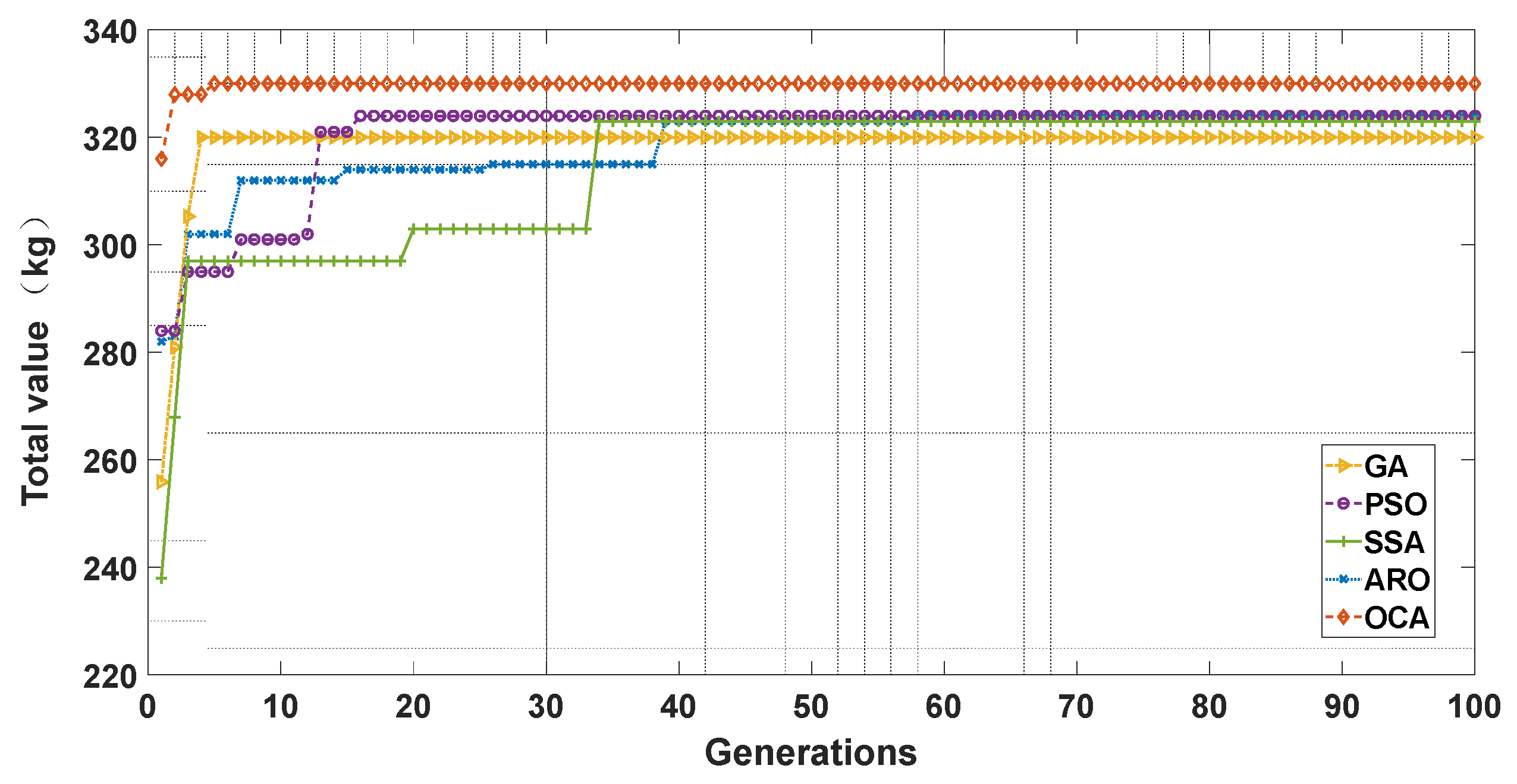
We randomly selected one experiment and plotted the convergence curve, as shown in Figure 6. We considered the value of items inside the knapsack as the fitness value of the function and aimed to find the maximum value as the search result. We can see that the OCA algorithm found the optimal result of 330 kg, while other algorithms did not find the optimal result in this search. The horizontal axis and the vertical axis represent the number of generations and the maximum value in the knapsack, respectively. We can see that although GA had a faster convergence speed than OCA, GA did not search for the optimal result in the fourth generation. OCA also had a very good convergence speed and converged in the fifth generation. PSO, SSA, and ARO converged only at 16, 34, and 39, respectively. The mechanisms of the determination of safety zones and zone competition in OCA accelerate the computational efficiency of the algorithm. Therefore, OCA exhibits a faster convergence rate.
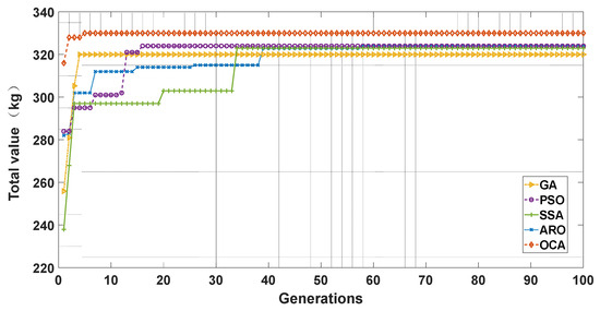
Figure 6.
Optimization evolution trajectories of GA, PSO, SSA, ARO, and OCA.
In Table 5, see a comparison of GA, PSO, SSA, ARO, and OCA over 500 Monte-Carlo trails. The average value reflects the overall performance of an algorithm. By comparing the average values, we can evaluate the relative efficiency of algorithms in solving the knapsack problem. OCA has the highest average value among all algorithms, indicating that OCA is more advantageous in addressing this problem. The standard deviation reflects the dispersion of data points, where a larger standard deviation indicates a wider range of variation in the data, while a smaller standard deviation suggests that the data is clustered more closely around the mean value, indicating a smaller range of variation. Therefore, the standard deviation can be used to evaluate the stability and predictability of data. OCA has the lowest standard deviation, indicating that it has better stability and consistency. The maximum value represents the quality of the optimal solution of the algorithm. OCA and ARO have both found the maximum value in the search for the knapsack problem. In solving the knapsack problem, a higher maximum value represents a better algorithm. The minimum value obtained by swarm intelligence algorithms for solving knapsack problems provides a measure of the worst-case solution found by the algorithm. From the table, it can be seen that the worst solution, 319, of OCA, is also higher than that of the other algorithms.
Table 5.
Total value and convergence generations of the GA PSO SSA ARO and OCA.
The proportion of the maximum value of the results of solving knapsack problems using swarm intelligence algorithms represents the proportion of the maximum value to the total solution space. A higher proportion of maximum values means that the algorithm can find solutions closer to the optimal solution more frequently when solving knapsack problems. This indicates that the algorithm has good performance, high searchability, and fast convergence. Regarding GA, PSO, and SSA, these three algorithms did not find the maximum value we know. The proportion of the maximum value of ARO is 40.00%, and the proportion of the maximum value of OCA is 65.71%, much higher than other values. The reasons are that the partition zones method can effectively reduce the dimension of the problem, the Oryctolagus cuniculus king maintenance mechanism ensures its stability, and the zone competition and predator killing accelerate its convergence speed. In summary, OCA, as a swarm intelligence algorithm, has broad application prospects in the field of problem-solving and optimization. Its unique search mechanism and adaptability enable it to effectively respond to challenges and perform tasks when solving complex problems, demonstrating excellent learning, optimization, and adaptability.
5. Conclusions
We propose the Oryctolagus cuniculus algorithm, which is inspired by the Oryctolagus cuniculi’s escape through caves in nature. Five mechanisms of Oryctolagus cuniculi are simulated by OCA, which are the determination of safety zones, the cave escape, the agglomeration of Oryctolagus cuniculi, the maintenance of the Oryctolagus cuniculus king, and the zone competition. We used empirical mode decomposition (EMD) to decompose the measured astronomical spectra, and the IMF obtained can be used to invert the measured reflectance template. We used OCA to screen IMFs, and finally realized the optimization of the template. We compared GA, PSO, SSA, ARO, and OCA. OCA has several advantages, including (1) faster convergence speed, (2) higher accuracy, (3) stronger stability, and (4) the ability to solve multidimensional problems. The reason is that the partition zones method can effectively reduce the dimension of the problem, the Oryctolagus cuniculus king maintenance mechanism ensures its stability, and the zone competition and predator killing accelerate its convergence speed.
To evaluate the performance of OCA, we investigated OCA with the zone competition mechanism and OCA without the zone competition mechanism. Only by combining OCA with the mechanism can we realize the global optimization of the algorithm. In addition, we compared OCA with GA, SSA, and ARO to demonstrate its superiority. To further investigate the generality of OCA, we extended its application to solve the 0-1 knapsack problem and compared the OCA with GA, PSO, SSA, and ARO. The experimental results show that the performance of OCA is more excellent than the comparison algorithms in terms of optimization effect, convergence rate, and optimization stability.
However, this algorithm has some drawbacks: the parameters of OCA are difficult to configure, and we require some key parameters to be set properly. OCA is likely to fall into a local optimum if the optimum is not initially divided into a safety zone. So, we also hope to do more optimization for this algorithm in the future. We will improve the search mechanism of the algorithm, introduce new change location methods and other methods to improve the performance and reliability of OCA, and strengthen the theoretical research and analysis of OCA. We derived and analysed it from the perspective of the mathematical model and explored the convergence and robustness of the algorithm.
Author Contributions
Conceptualization, D.J.; methodology, J.L.; Polish, Z.K.; software, Z.Z.; validation, X.M.; writing—original draft preparation, D.J.; writing—review and editing, D.J. All authors have read and agreed to the published version of the manuscript.
Funding
The authors disclosed receipt of the following financial support for the research, authorship, and/or publication of this article: This study was supported by the National Natural Science Foundation of China (Nos. 61873196, 62373030, 61772187), the Postgraduate Innovation and Entrepreneurship Foundation of Wuhan University of Science and Technology (No. JCX2022078), and the Innovation Program for Quantum Science and Technology under Grant (No. 2021ZD0303400).
Institutional Review Board Statement
Not applicable.
Informed Consent Statement
Not applicable.
Data Availability Statement
Publicly available datasets were analyzed in this study. This data can be found here: [https://www.eso.org/public/].
Conflicts of Interest
The authors declare no conflict of interest.
References
- Wang, L.; Cao, Q.; Zhang, Z.; Mirjalili, S.; Zhao, W. Artificial rabbits optimization: A new bio-inspired meta-heuristic algorithm for solving engineering optimization problems. Eng. Appl. Artif. Intell. 2022, 114, 105082. [Google Scholar] [CrossRef]
- Holland, J.H. Adaptation in Natural and Artificial Systems: An Introductory Analysis with Applications to Biology, Control, and Artificial Intelligence, 3rd ed.; University of Michigan Press: Ann Arbor, MI, USA, 1975; pp. 27–67. [Google Scholar]
- Storn, R.; Price, K. Differential Evolution—A Simple and Efficient Heuristic for Global Optimization over Continuous Spaces. J. Glob. Optim. 1995, 11, 341–359. [Google Scholar] [CrossRef]
- Bäck, T. Evolution strategies: An alternative evolutionary algorithm. In Lecture Notes in Computer Science, Proceedings of the European Conference on Artificial Evolution, Brest, France, 4–6 September 1995; Alliot, J.-M., Lutton, E., Ronald, E., Schoenauer, M., Snyers, D., Eds.; Springer: Berlin/Heidelberg, Germany, 1996. [Google Scholar]
- Mirjalili, S.; Mirjalili, S.M.; Lewis, A. Queen bee evolution for numerical function optimization. Appl. Soft Comput. 2015, 30, 1–13. [Google Scholar]
- Kennedy, J.; Eberhart, R. Particle swarm optimization. In Proceedings of the ICNN’95-International Conference on Neural Networks, Perth, WA, Australia, 27 November 1995. [Google Scholar]
- Yang, X.S. Firefly Algorithms for Multimodal Optimization. In Stochastic Algorithms: Foundations and Applications. SAGA 2009, Proceedings of the 5th International Symposium on Stochastic Algorithms, Sapporo, Japan, 26–28 October 2009; Watanabe, O., Zeugmann, T., Eds.; Springer: Berlin/Heidelberg, Germany, 2009. [Google Scholar]
- Mirjalili, S.; Lewis, A. The whale optimization algorithm. Adv. Eng. Softw. 2016, 95, 51–67. [Google Scholar] [CrossRef]
- Wang, X. Artificial fish swarm algorithm: A new optimization technique. Appl. Math. Comput. 2004, 148, 649–664. [Google Scholar]
- Karaboga, D. An Idea Based on Honey Bee Swarm for Numerical Optimization. Inf. Sci. 2006, 176, 937–961. [Google Scholar]
- Peng, J.; Li, X.; Liu, B. A New Optimization Algorithm Inspired by the Cuckoo Behavior. Neural Process. Lett. 2016, 44, 487–502. [Google Scholar]
- Mellal, M.A. Virus colony search: A new bio-inspired optimization algorithm. Neural Comput. Appl. 2014, 24, 1847–1864. [Google Scholar]
- Mirjalili, S. The Harris hawk optimization algorithm. Neural Comput. Appl. 2019, 31, 6751–6773. [Google Scholar]
- Chen, J.; Wang, Y.; Zhang, S.; Li, X. Artificial rabbit optimization algorithm: A new metaheuristic algorithm. Soft Comput. 2019, 23, 5433–5449. [Google Scholar]
- Kirkpatrick, S.; Gelatt, C.D., Jr.; Vecchi, M.P. Optimization by simulated annealing. Science 1983, 220, 671–680. [Google Scholar] [CrossRef] [PubMed]
- Esmaili, P.; Mohanna, S. A novel heuristic optimization method: Gravitational search algorithm. In Proceedings of the International Conference on Machine Learning and Cybernetics, Kunming, China, 12 July 2008. [Google Scholar]
- Liu, K.M.; Lam, J.; Wu, Z.F.; Wu, X.Y. A novel optimization method: Artificial chemical reaction optimization. Nat. Comput. 2005, 8, 275–278. [Google Scholar]
- Li, B.C.; He, K.; Hu, Q.N. Water cycle algorithm: A novel metaheuristic optimization method for solving constrained optimization problems. J. Hydrol. 2014, 513, 355–366. [Google Scholar]
- Chen, H.; Long, H.; Fang, H. An Optimization Method Based on Particle Collisions. Control Decis. 2009, 24, 1452–1456. [Google Scholar]
- Yang, X.S.; Gandomi, A.H.; Karamanoglu, M. Galaxy-based search algorithm for global optimization. Appl. Soft Comput. 2016, 40, 249–259. [Google Scholar]
- Shojafar, M.; Gandomi, A.H.; Cordeschi, N.; Abawajy, J. Henry gas solubility-based optimization algorithm for task scheduling in cloud computing. Neural Comput. Appl. 2016, 27, 2051–2064. [Google Scholar]
- Mirjalili, S. Charged system search for solving non-convex optimization problems. Eng. Softw. 2015, 83, 49–59. [Google Scholar]
- Rao, R.V.; Savsani, V.J.; Vakharia, D.P. Teaching-Learning-Based Optimization: An Optimization Method for Continuous Non-Linear Large Scale Problems. Int. J. Comput. Sci. Issues 2011, 8, 63–69. [Google Scholar] [CrossRef]
- Yang, X.S.; Deb, S.; Fong, S.J. Social and cultural algorithm for global optimization. J. Comput. Theor. Nanosci. 2013, 10, 877–886. [Google Scholar]
- Yang, X.S.; Deb, S.; Wang, X.S. Focus group optimization: A nature-inspired optimization algorithm for global optimization. Inf. Sci. 2016, 345, 340–354. [Google Scholar]
- Mirjalili, S. Poverty and richness-based evolutionary algorithm: A novel approach for global optimization. Neural Comput. Appl. 2015, 27, 495–513. [Google Scholar] [CrossRef]
- Yang, X.S.; Liu, D.; Jia, S. League championship algorithm: A new algorithm for numerical function optimization. Soft Comput. 2017, 21, 6969–6983. [Google Scholar]
- Mirjalili, S.; Mirjalili, S.M.; Lewis, A. Student psychological-based optimization: A novel learning algorithm. Neural Comput. Appl. 2017, 28, 4141–4159. [Google Scholar]
- Yang, X.S.; Karamanoglu, M.; He, X. Tug of war optimization: A new method for global optimization. Soft Comput. 2017, 21, 5227–5241. [Google Scholar]
- Mirjalili, S. Human mental search algorithm: A new optimization algorithm inspired by human cognition. Adv. Eng. Softw. 2016, 102, 58–69. [Google Scholar]
- Mirjalili, S.; Mirjalili, S.M.; Hatamlou, A. Stochastic paint optimizer: A novel optimization algorithm. Appl. Soft Comput. 2017, 56, 460–473. [Google Scholar]
- Yang, X.S.; Gandomi, A.H.; Karamanoglu, M. Supply-demand optimization: A new nature-inspired optimization algorithm. IEEE Trans. Cybern. 2018, 49, 2377–2389. [Google Scholar]
- Mirjalili, S. Imperialist competitive algorithm: An algorithm for optimization inspired by imperialistic competition. Inf. Sci. 2016, 341, 19–33. [Google Scholar]
- Yang, X.S.; Gandomi, A.H.; Talatahari, S.; Deb, S. Soccer league competition algorithm: A novel nature-inspired optimization algorithm. Soft Comput. 2018, 22, 741–763. [Google Scholar]
- Elaziz, M.A.; El-Samie, F.E.A. Sparrow search algorithm: A novel swarm intelligence optimization technique. Neural Comput. Appl. 2016, 27, 1771–1785. [Google Scholar]
- Wang, Y.D.; Zheng, W.; Zhang, S. Review of X-ray pulsar spacecraft autonomous navigation. arXiv 2023, arXiv:2304.04154. [Google Scholar] [CrossRef]
- Wang, Y.D.; Zhang, S.N.; Ge, M.Y. Fast on-orbit pulse phase estimation of X-ray Crab pulsar for XNAV flight experiments. IEEE Trans. Aerosp. Electron. Syst. 2023, 59, 3395–3404. [Google Scholar] [CrossRef]
- Liu, J.; Wang, Y.D.; Ning, X.L.; Hu, J.T. Two-dimensional Doppler velocimetry approach using a single X-ray pulsar for Jupiter exploration. Acta Astronaut. 2023, 213, 373–384. [Google Scholar] [CrossRef]
- Liu, J.; Fang, J.C.; Yang, Z.H.; Kang, Z.W.; Wu, J. X-ray pulsar/Doppler difference integrated navigation for deep space exploration with unstable solar spectra. Aerosp. Sci. Technol. 2015, 41, 144–150. [Google Scholar] [CrossRef]
- Liu, J.; Wang, T.; Ning, X.L.; Kang, Z.W. Modelling and analysis of celestial Doppler difference velocimetry navigation considering solar characteristics. IET Radar Sonar Navig. 2020, 14, 1897–1904. [Google Scholar] [CrossRef]
- Liu, J.; Li, Y.Y.; Ning, X.L.; Chen, X.; Kang, Z.W. Modeling and analysis of solar Doppler difference bias with arbitrary rotation axis. Chin. J. Aeronaut. 2020, 33, 3331–3343. [Google Scholar] [CrossRef]
- Liu, J.; Ning, X.L.; Ma, X.; Fang, J.C. Geometry error analysis in solar Doppler difference navigation for the capture phase. IEEE Trans. Aerosp. Electron. Syst. 2019, 55, 2556–2567. [Google Scholar] [CrossRef]
- Llobat, L.; Marín-García, P.J. Application of protein nutrition in natural ecosystem management for European rabbit (Oryctolagus cuniculus) conservation. Biodivers. Conserv. 2022, 31, 1435–1444. [Google Scholar] [CrossRef]
- Zhang, J.; Liu, J.; Ma, X.; Kang, Z.W.; Wang, Z.N. Real-time and highly accurate solar spectrum velocimetry using the mirror NDFT-CS for Doppler navigation. J. Aerosp. Eng. 2021, 34, 04021091. [Google Scholar] [CrossRef]

Disclaimer/Publisher’s Note: The statements, opinions and data contained in all publications are solely those of the individual author(s) and contributor(s) and not of MDPI and/or the editor(s). MDPI and/or the editor(s) disclaim responsibility for any injury to people or property resulting from any ideas, methods, instructions or products referred to in the content. |
© 2023 by the authors. Licensee MDPI, Basel, Switzerland. This article is an open access article distributed under the terms and conditions of the Creative Commons Attribution (CC BY) license (https://creativecommons.org/licenses/by/4.0/).