Abstract
This paper proposes a dynamic phase comparison algorithm for planar direction finding on a high-speed moving satellite radio receiver, treating the moving antenna as equivalent to single-baseline array antennas. Based on a phase interferometer algorithm, this algorithm adjusts the baseline length according to the frequency measurement module and the satellite’s high-speed motion to avoid phase ambiguity indirectly. By integrating the traditional amplitude comparison algorithm based on orthogonal dipole antennas, a dynamic fusion direction-finding method is proposed. Simulations demonstrate that this approach method not only covers a broader range of direction finding but also achieves higher accuracy, providing valuable insights for acquiring three-dimensional plasmagrams with space-borne plasma imagers.
1. Introduction
The understanding of the ionosphere began with ground-based ionosondes producing frequency–height charts. With the advancement of modern electronic technology, techniques for detecting space plasma environments have also gradually developed. As satellite technology evolved, various countries launched space-borne instruments to explore the space environment [1,2,3,4,5,6,7,8], further investigating the Earth’s plasma layer and magnetosphere and even the Martian space environment [9]. Among them, space-borne instruments such as RPI (radio plasma imager), DSX, PWE, and PWI use orthogonal dipole antennas to receive or transmit EM waves (electromagnetic waves) within a VLF (very-low frequency) to VHF (very-high frequency) range.
RPI [2] is the first space-borne radio plasma imager with both active and passive detection capabilities launched by NASA. Active detection focuses on using space plasma echo reflections to determine plasma electron density distributions. Passive detection mainly observes ionospheric whistle waves, hiss waves, etc. The total frequency range covered by the receiver in both modes is 3 kHz–3 MHz. Additionally, the maximum detection range of the RPI is up to 4 , which can be considered the far field for received EM waves. Equipped with a three-channel VLF receiver and tri-orthogonal dipole antennas, it can perform direction finding of EM waves using the amplitude comparison algorithm [10] and MUSIC algorithm [11]. The amplitude comparison algorithm used by RPI for direction finding has a range of only 0° to 90°, leading to angle ambiguity in spatial direction finding.
The phase interferometer algorithm uses array antennas to determine the direction of EM waves. Due to the higher measurement accuracy, it is widely adopted in DF (direction finding) systems. The power of the interferometer system is particularly evident in radio astrometry and geodesy [12], which is also used for observing stations to explore the distribution of radio sources on the solar disk [13].
Early in the study of the ionosphere, researchers began using interferometers to estimate the DOA (direction of arrival) of electromagnetic echoes [14,15,16]. EM waves in the far field can be considered parallel waves. When EM waves from different directions arrive at antennas located at different positions, there is a phase difference in the signals received at the same moment due to their different locations. By analyzing the phase difference between any two received signals, the azimuth angle of the EM waves can be determined, thereby obtaining the direction of the radiation source. Due to the phase ambiguity in interferometers [17], researchers have conducted in-depth research over the years to resolve this ambiguity [18,19,20,21,22,23]. In the context of space-borne receivers, several researchers have proposed rotational baseline disambiguation methods based on the spinning motion of satellites [24,25].
Hence, to improve the DF system performance of the satellite radio receiver, this paper proposes a dynamic phase comparison algorithm against the backdrop of a high-speed moving satellite based on the phase interferometer algorithm. This algorithm, while offering a broader DF range than the amplitude comparison algorithm, dynamically calculates and adjusts the baseline length to avoid phase ambiguity. By integrating the amplitude comparison algorithm, it further achieves the purpose of improving DF accuracy.
2. Description of the Algorithm
2.1. Dynamic Phase Comparison Algorithm
The dynamic phase comparison algorithm is based on the phase interferometer algorithm. In the interferometer DF system, as shown in Figure 1, it is accomplished using array antennas consisting of at least two antennas.
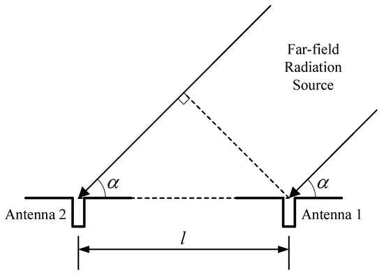
Figure 1.
Principle of the phase interferometer algorithm.
Assume that single-tone plane EM waves emitted from a far-field radiation source propagate to a single-baseline array antennas. Due to the time difference between the signals received by the two antennas, there is a phase difference between them. In this way, the azimuth angle of the EM waves, defined as the angle between the direction of the EM waves and the baseline of array antennas, can determine the phase difference
where c is the speed of light; l is the distance between the antennas, as known as the baseline length of the interferometer; and and f are the wavelength and frequency of the EM waves. If l and f are known, the azimuth angle of the radiation source signal can be determined as
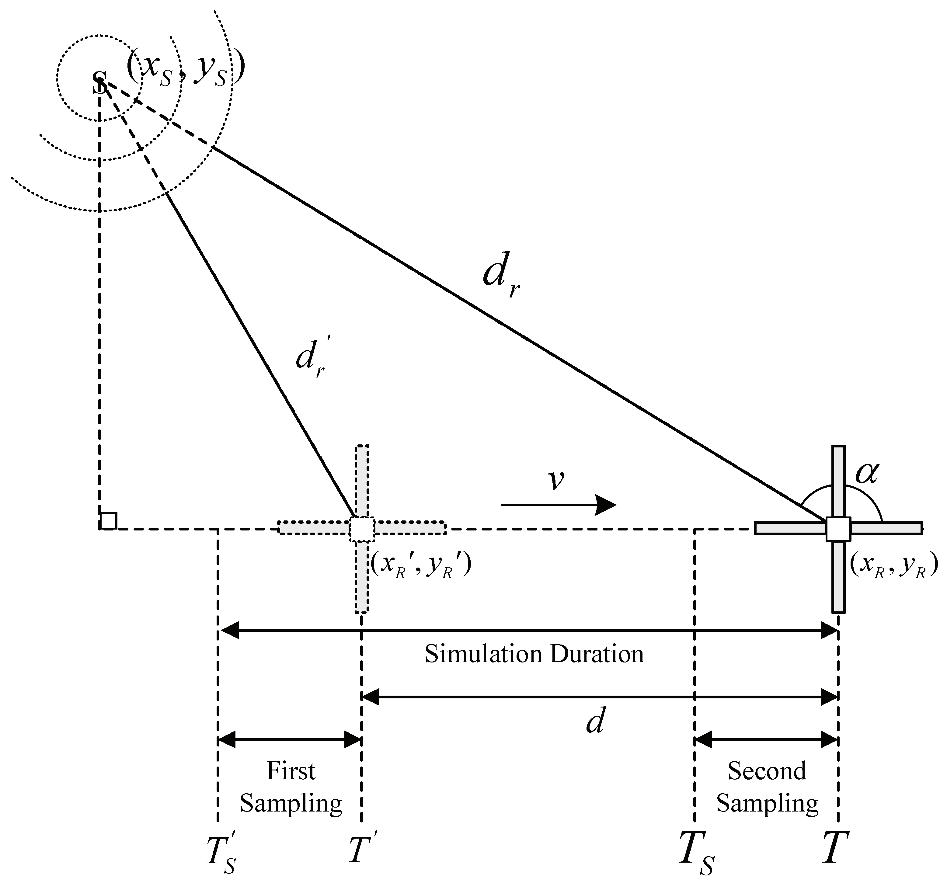
Compared with the phase interferometer algorithm, the dynamic phase comparison algorithm does not use array antennas. Instead, it employs a single antenna element receiving signals under high-speed uniform motion. As shown in Figure 2, if the radiation source continuously emits EM waves periodically for a certain period, it can be considered as two (or more) virtual antenna elements during the high-speed uniform motion on the satellite, thereby achieving signal reception and sampling at different positions.
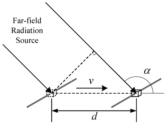
Figure 2.
Principle of the dynamic phase comparison algorithm.
During the process where a far-field radiation source emits single-tone EM waves periodically for a certain period, a satellite receiver equipped with a dipole antenna and a single-channel receiver move at a high velocity v. Considering that the plane waves are emitted by the far-field radiation source, the two receptions of EM waves are treated as parallel waves with constant frequency. Respectively, the signals sampled by the satellite receiver are and at two different times, and T. From Equation (1), the phase difference caused by the angle between the direction of the EM waves can be known.
Assume the position of the radiation source remains constant and ignore the short movement of the receiver during the brief signal sampling period. Then, the signals received at two different positions can be approximately represented as
where is the time difference experienced by the moving satellite and K is the antenna gain.
Hence, the total phase difference between the received signals and consists of two parts: one part is due to the time difference between the two receptions of the signal by the satellite receiver; and the other part is due to the angle between the direction of the satellite’s motion and the incoming direction of the EM waves, which also causes a phase difference in the signals. Thus, the total phase difference can be approximately obtained as
Based on the principles of the phase interferometer algorithm from Equation (2), the azimuth angle of the radiation source signal can be obtained as
where d is the distance covered by the satellite during its high-speed motion between the two signal receptions, which can be obtained from the satellite’s velocity v and . The expression for the satellite’s motion distance is
By combining the above expressions, the azimuth angle of the radiation source signal can be obtained as
where the range of values for the phase difference and signal azimuth angle are
2.2. Accuracy Analysis
The dynamic comparison phase algorithm, based on the phase interferometer algorithm, treats the distance traveled by the satellite as equivalent to the baseline length. To perform an accuracy analysis of the dynamic comparison phase algorithm, a total differential of Equation (7) is carried out, which can be obtained as
By applying the chain rule to solve for the three partial derivatives, the results can be obtained as
where
Hence, the total differential can be obtained as
Analyzing the total differential equation reveals:
- From Equation (10), when the frequency of the EM waves or the satellite motion distance is relatively small, the azimuth accuracy is significantly influenced by the measurement accuracy of the phase difference.
- From Equation (11), the azimuth accuracy is more greatly affected by the measurement accuracy of the frequency of the EM waves, especially when the absolute value of the phase difference is large (i.e., when is close to 0° or 180°) or when the satellite motion distance is small. The frequency appears in the form of , which impacts the azimuth accuracy more.
- From Equation (12), the azimuth accuracy is more significantly influenced by the measurement accuracy of the satellite motion distance, particularly when the absolute value of the phase difference is large (i.e., when is close to 0° or 180°) or when the frequency of the EM waves is low. The distance appears in the form of , which also impacts the azimuth accuracy more.
Given that the measurement error of phase difference significantly impacts the DF error, and because obtaining the azimuth angle from the phase difference is a nonlinear transformation, the effect of different EM waves azimuth angles on the phase difference cannot be ignored. The following analysis of the measurement accuracy of phase difference involves performing a total differential of the equation, which can be obtained as
The analysis of the equation reveals that the measurement error in phase difference originates from the measurement errors in the frequency of the EM waves and baseline length. Specifically, the impact of errors is more significant when the azimuth angle of the EM waves is close to the orientation of the baseline (i.e., when is close to 0° or 180°).
In summary, when designing and applying the dynamic comparison phase DF system, special attention should be paid to the following three core elements to ensure that the DF accuracy meets requirements:
- Improving the measurement accuracy of the phase difference is key to enhancing the performance of the phase comparison algorithm. Accurate measurement of the phase difference can effectively reduce DF errors.
- The satellite motion distance (i.e., the baseline length) should be sufficiently large to provide higher DF accuracy when direction finding is performed on VLF signals.
- In the practical application of the phase comparison algorithm, the DF accuracy is more sensitive when the azimuth angle is close to 0° and 180°, making it more susceptible to other measurement errors.
2.3. Phase Ambiguity
In the process of direction finding using both the phase interferometer algorithm and the dynamic phase comparison algorithm, the phase difference between the signals received by the moving receiver twice is periodic with a cycle of . However, the phase difference between the two signals is measured modulo within the range of . If the actual phase difference exceeds this range, these DF algorithms will experience ambiguity in the phase calculation process.
If the actual phase difference is given by
where N represents the phase ambiguity number and , then the unambiguous azimuth angle range for the DF system is
From the equation, it is evident that to expand the DF range of the comparison phase system, it is necessary to shorten the baseline length. However, this requirement contradicts the need to improve DF accuracy.
Hence, in the phase interferometer algorithm, there is an inherent contradiction between the DF accuracy and the maximum unambiguous angle. To overcome this issue, multi-baseline configurations are typically adopted, including the use of long and short baselines, virtual baselines, and other disambiguation algorithms [18,19,21,22,23]. In practical applications, the method of combining long and short baselines for VLF signals has specific limitations. Firstly, for VLF signals, the wavelength is very long. Such long baselines not only make the computational load relatively large when using multi-baseline disambiguation algorithms but also increase the system’s complexity. Secondly, long baselines pose certain challenges for the installation locations of ground-based DF array antennas and are even more difficult to implement in space-borne plasma imager DF systems.
However, in the dynamic comparison phase algorithm, its principle takes advantage of the high-speed motion of satellites to be equivalent to the array antennas, with the interferometer baseline length determined by the velocity of the satellite and the time difference between two signal receptions. Hence, in the process of dynamic direction finding, after completing the first signal reception, the corresponding maximum baseline length can be calculated through the measurement capability of the target signal frequency. Then, based on the velocity of the satellite, the required time interval for the second signal reception is directly calculated, thus achieving the maximum DF accuracy under the condition of phase ambiguity elimination.
2.4. Angular Ambiguity
In both the phase interferometer algorithm and the dynamic phase comparison algorithm, the final DF angle range is . Because the DF angle is the angle between the azimuth and the interferometer baseline, in planar direction finding, there is a possibility of having two possibilities for the DF result, corresponding to and .
Figure 3 shows the antenna coordinate system of RPI, which is equipped with tri-orthogonal dipole antennas and a three-channel receiver. Moreover, RPI uses the amplitude comparison algorithm in the DF system.
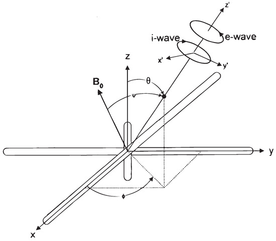
Figure 3.
Antenna coordinate system of the RPI (radio plasma imager) [10].
The direction of the EM waves can be obtained by comparing the intensity of the signals received by the three antennas. The expressions for the azimuth angle and elevation angle are given by [10]
where is the azimuth angle and is the elevation angle. The range of values for both angles is, respectively,
In the amplitude comparison algorithm, the key to determining the arrival angle of EM waves lies in analyzing the ratio of signal amplitudes received by tri-orthogonal dipole antennas. Because signal amplitudes cannot be negative, the determination of the DF angle is subject to angular ambiguity.
Taking the planar amplitude comparison algorithm as an example, when the actual arrival angle of the EM waves is , , , or , the DF results obtained by this algorithm will not be able to distinguish between these four possibilities. Similarly, in the spatial amplitude comparison DF system, there are eight different possibilities for the result. Although the amplitude comparison algorithm can provide an estimate of the arrival angle, it has a angular ambiguity in signal direction finding.
Hence, introducing the dynamic phase comparison algorithm into the DF system on a space-borne plasma radio imager can achieve a larger effective DF range with high accuracy. This will be further discussed in the following section.
3. Simulation Results and Analysis
In this section, several simulations of DF algorithms are conducted to compare and analyze their accuracy under various influencing factors. The simulations employed plain numerical methods and generated normally distributed random numbers to add additive Gaussian noise to the signal.
Initially, a planar simulation of the dynamic phase comparison algorithm proposed in the previous section is carried out, which is based on a satellite receiver equipped with a dipole antenna. Next, based on the receiver equipped with dual orthogonal dipole antennas, the dynamic phase comparison algorithm is simulated alongside the planar amplitude comparison algorithm to analyze the DF accuracy under different expected angles. Subsequently, by integrating the amplitude comparison algorithm into the dynamic phase comparison algorithm, a dynamic fusion DF method is proposed. Additionally, by incorporating digital signal processing techniques, including band-pass filtering and coherent accumulation, a dynamic fusion DF system for space-borne digital receivers is designed. Finally, considering three influencing factors: SNR, sampling frequency, and coherent accumulation, the performance of the DF system is analyzed through three simulations.
3.1. Dynamic Phase Comparison Algorithm
For the simulation of the dynamic comparison phase algorithm, as shown in Figure 4, consider the following default simulation parameters as described: Considering that the frequency range of the RPI receiver is 3 kHz–3 MHz, S represents a far-field radiation source that continuously emits a 32 kHz sine wave signal. It is also assumed that the final distance between the satellite and the far-field radiation source is 20 times the wavelength of the EM waves. A satellite receiver equipped with a dipole antenna completes its first signal sampling during the period from to , and its half-wavelength distance is calculated and set as the satellite motion distance d between the two samplings. Then, the receiver completes the second signal sampling during the same period. Ultimately, the DF system utilizes the dynamic phase comparison algorithm to complete the radiation source direction finding.

Figure 4.
Simulation of the dynamic phase comparison algorithm.
The single simulation result of the dynamic phase comparison algorithm, as illustrated in Figure 5, shows that with an SNR of 10 dB and a receiver sampling rate of 6.4 MHz, each sampling of one cycle signal is completed for phase comparison. From the figure, it is evident that the algorithm tends to produce significant errors mainly near 0° and 180°, which aligns with the conclusions of the accuracy analysis in Section 2.2. The reason for this phenomenon is due to the adjacent phase differences of and . When subject to disturbances from noise and other factors, it is easy for the measured phase difference to undergo abrupt changes, directly causing substantial DF errors near 180°.
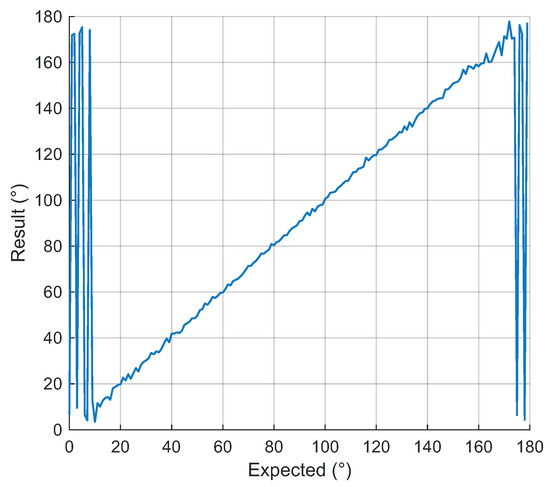
Figure 5.
Simulation result of the dynamic phase comparison algorithm.
From the precision analysis in Section 2.2, it is understood that the measurement of phase difference is a very important metric in the dynamic phase comparison algorithm. However, the phase difference is easily disturbed by various factors, such as noise, the sampling rate of the radio receiver, and the length of the comparison signal.
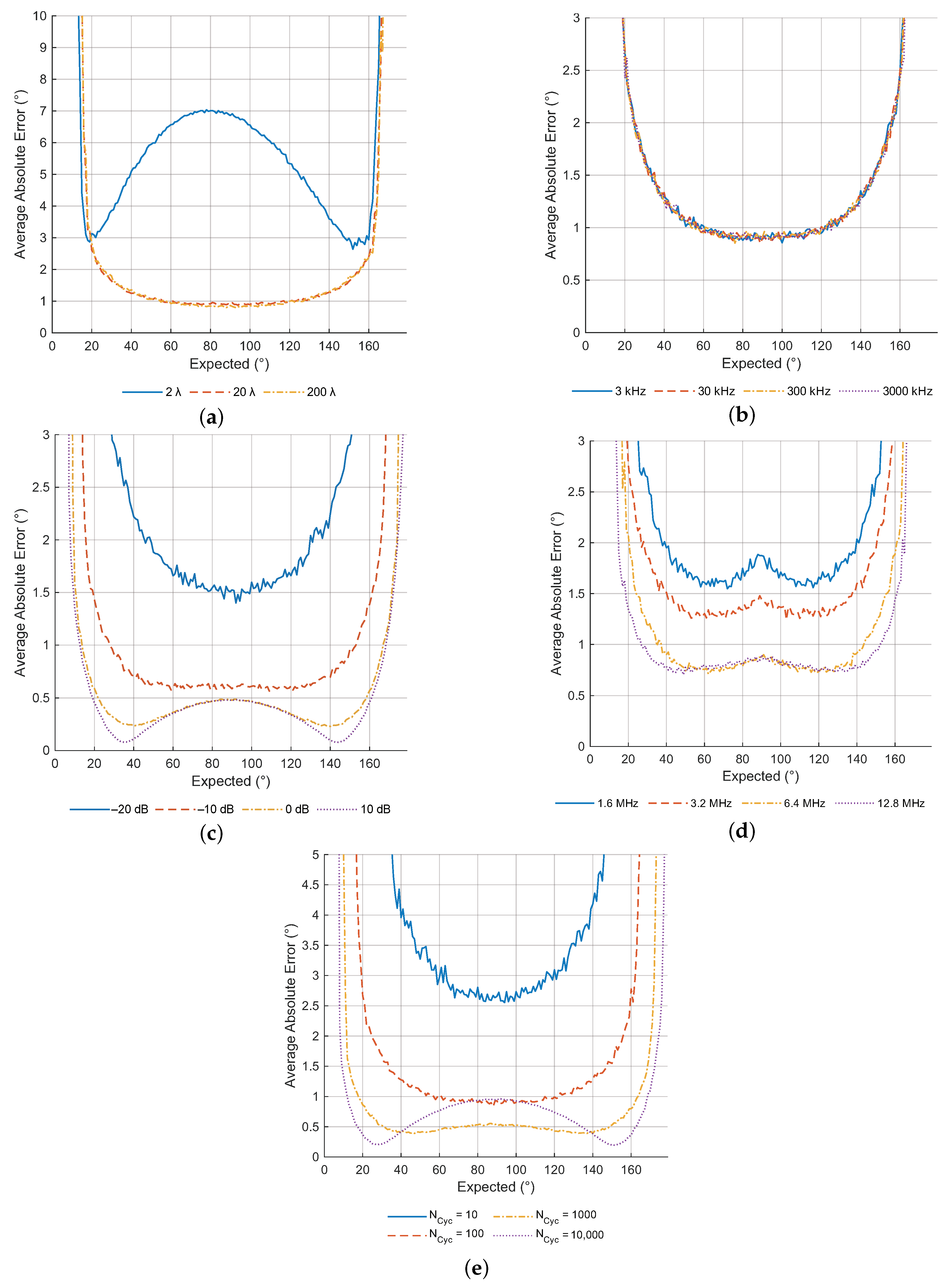
Figure 6 shows the curves of the average absolute error from one thousand simulations of the algorithm, influenced by five factors: relative distance, signal frequency, SNR, the sampling rate of the receiver, and the length of the received signal. In the simulations, the default parameter settings are as follows: an SNR of −15 dB, a receiver sampling rate of 6.4 MHz, and the receiver sampling duration for each sampling is 100 cycles of the EM waves signal.
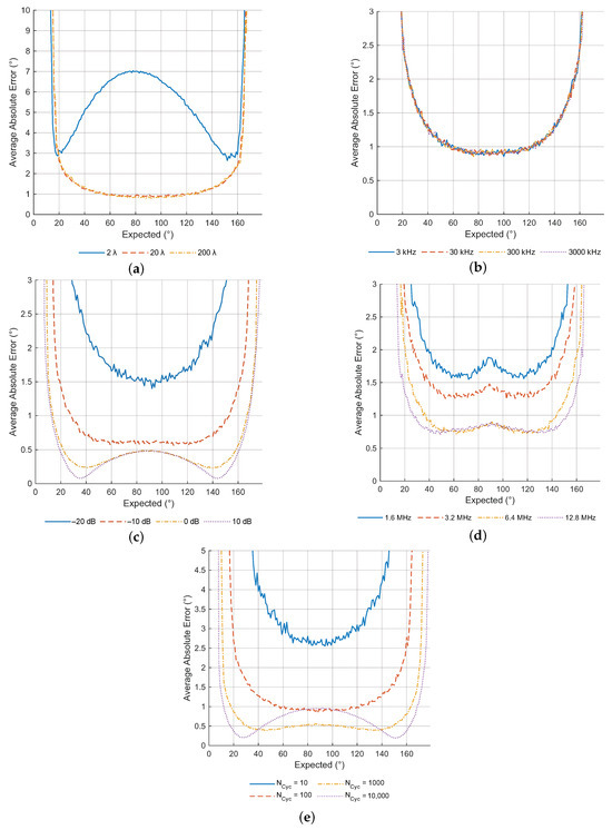
Figure 6.
Average absolute error of the dynamic phase comparison algorithm under different (a) relative distances, (b) signal frequencies, (c) SNRs, (d) receiver sampling rates, and (e) numbers of received signal cycles.
The analysis of the simulation results reveals that the relative distance, SNR, the sampling rate of the receiver, and length of the comparison signal all have a significant impact on the algorithm. From the analysis, the following conclusions can be drawn:
- Generally, the lower the relative distance, the higher the SNR, the higher the sampling rate, or the longer the signal length, the higher the DF accuracy;
- Compared with the almost identical DF accuracy for far-field radiation sources, the algorithm exhibits lower DF accuracy for near-field sources. When the ratio of relative distance to wavelength is fixed, the DF accuracy for radiation sources of different frequencies remains essentially consistent;
- Azimuth angles of EM waves near 0° and 180° are likely to produce significant DF errors, and the error may also increase near 90°;
- The length of the comparison signal should not be too long as it may lead to a decrease in DF accuracy. Especially when approaching 90°, overly long signals can cause larger errors.
3.2. Comparison of the Dynamic Phase Comparison and the Amplitude Comparison Algorithms
From Section 2.4, it is evident that both the dynamic phase comparison algorithm and the amplitude comparison algorithm face different angular ambiguity issues, with the former offering a larger DF range. Moreover, simulation results from the previous subsection indicate that the dynamic phase comparison algorithm exhibits lower DF accuracy near azimuth angles of 0°, 90°, and 180°. Therefore, it might be beneficial to consider integrating the traditional amplitude comparison algorithm to analyze DF results at different angles with those of the dynamic phase comparison algorithm. This integration could improve DF accuracy while expanding the DF range.
Taking the example of a satellite receiver equipped with a dual orthogonal dipole antennas and two-channel receiver, this section conducts a simulation of the two algorithms during satellite motion. Based on the simulation from the previous subsection, the antenna on the satellite receiver is changed to a dual orthogonal dipole antenna. As shown in Figure 7, it is assumed that the two antennas are aligned with the X-axis and Y-axis directions in the coordinate system, respectively. The satellite moves in the positive direction of the X-axis during the short-term DF process.

Figure 7.
Simulation of the two DF algorithms.
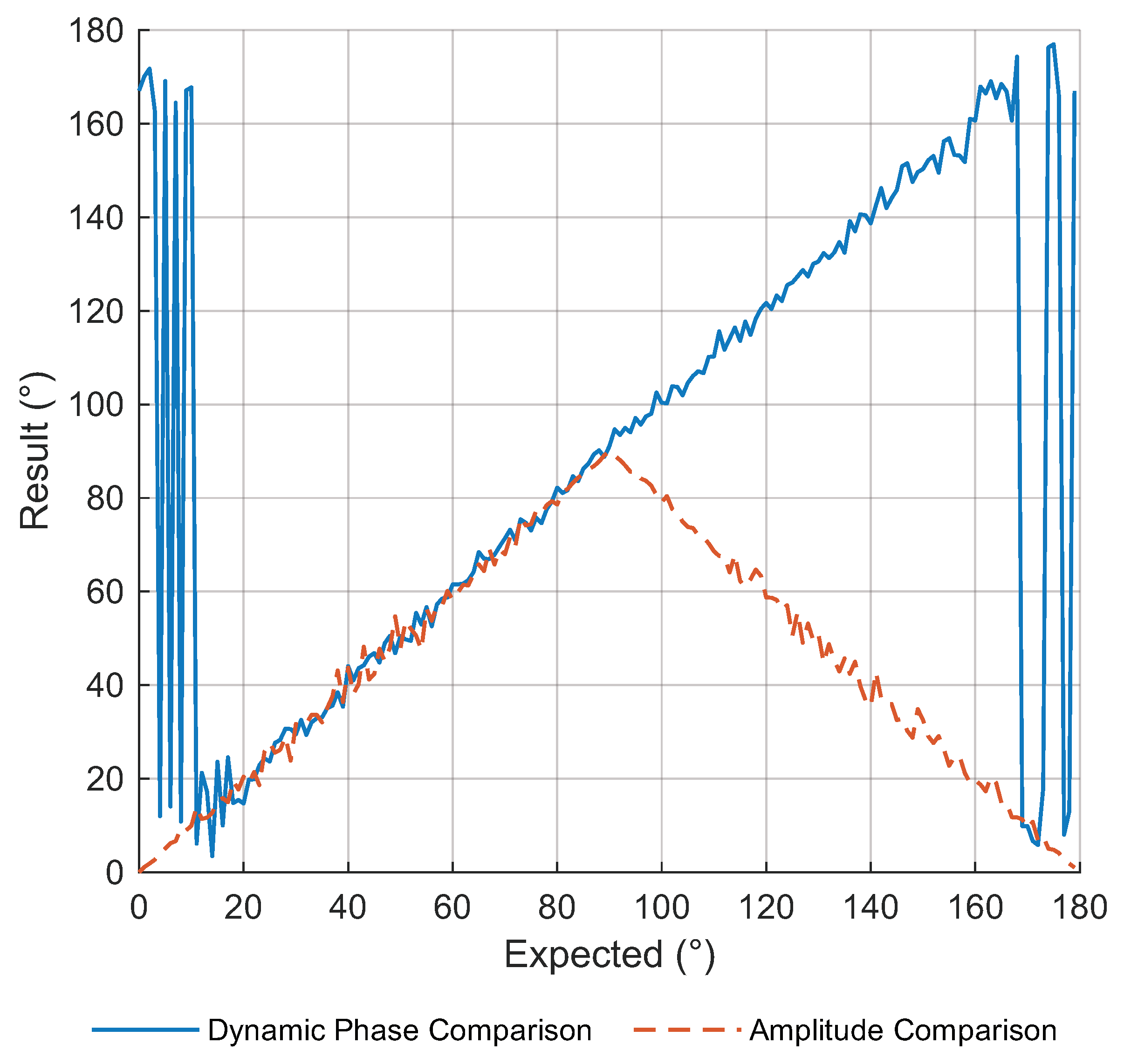
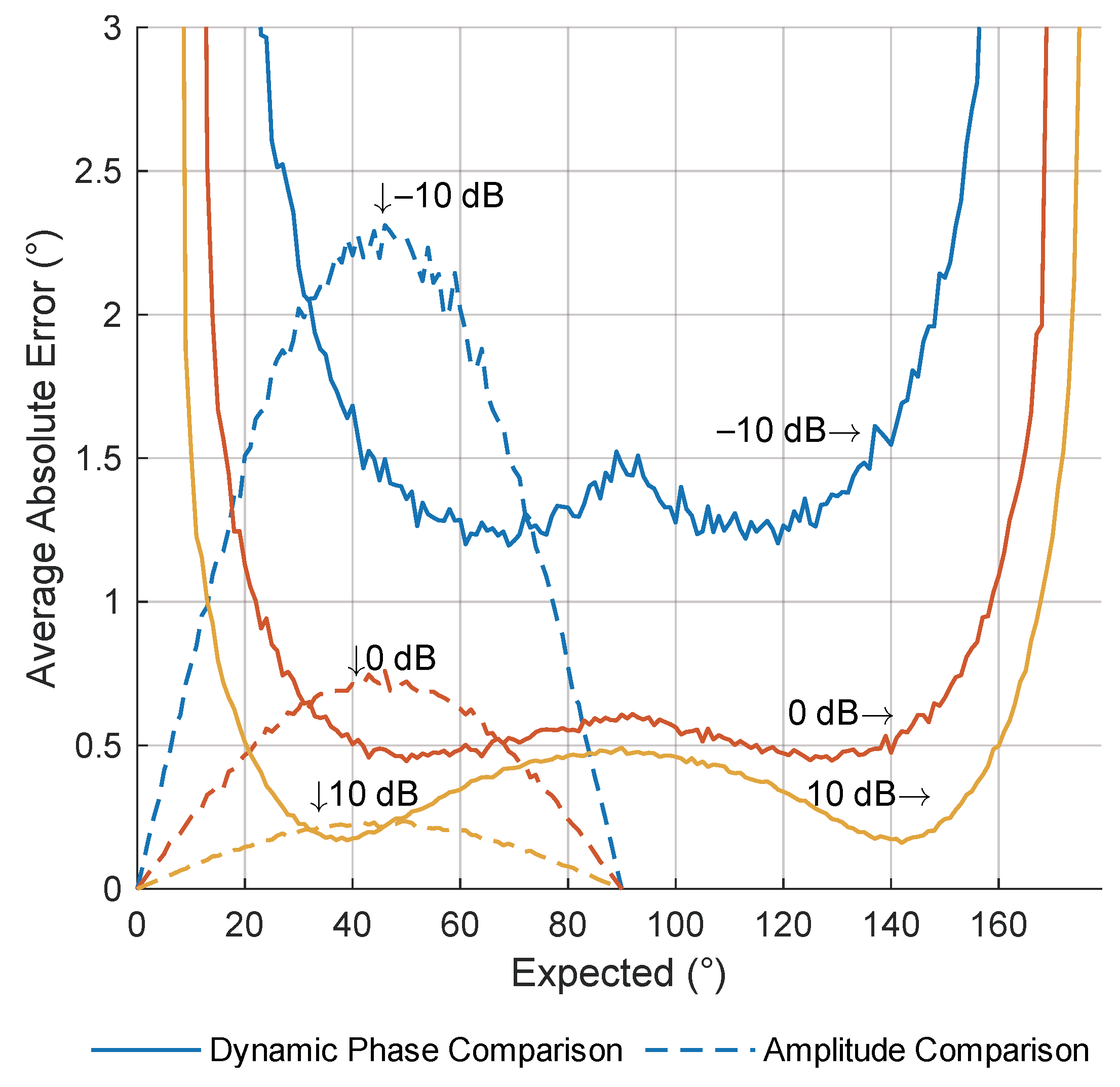
The simulation parameters are set with an SNR of −10 dB and a receiver sampling rate of 6.4 MHz, and each sampling involves 10 cycles of the signal. Figure 8 shows the one simulation result of the two direction-finding algorithms, and Figure 9 shows the average absolute error curves from one thousand simulations under three different SNR conditions. The amplitude comparison algorithm only calculates errors below 90°.
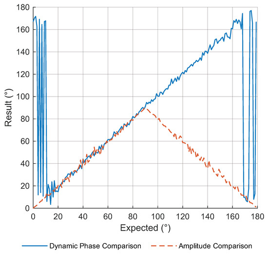
Figure 8.
One simulation result of the dynamic phase comparison algorithm and the amplitude comparison algorithm.
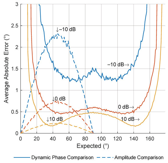
Figure 9.
Average absolute error of the dynamic phase comparison algorithm and the amplitude comparison algorithm under different SNRs.
The simulation results indicate that when the azimuth angle is within the range of approximately 30° to 80°, the dynamic phase comparison algorithm generally exhibits relatively high accuracy; meanwhile, the amplitude comparison algorithm shows relatively high accuracy when the azimuth angle is close to 0° and 90°.
Hence, by integrating these two DF algorithms, it is possible to further improve DF accuracy with the higher DF range.
3.3. Dynamic Fusion Direction Finding Method
In this subsection, we attempt to integrate the amplitude comparison algorithm into the dynamic phase comparison algorithm to improve accuracy when the azimuth angle is close to 0°, 90°, and 180°.
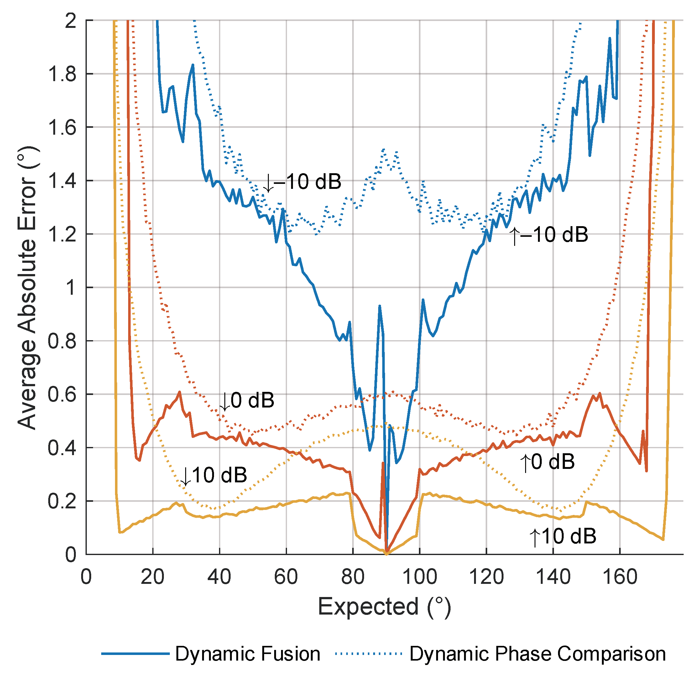
Figure 10 shows the average absolute error curves from one thousand simulations for both the dynamic fusion DF method and the dynamic phase comparison algorithm. Table 1 provides an analysis of the simulation results in terms of improvements in DF accuracy. The simulation parameters remain consistent with those outlined in the previous subsection.
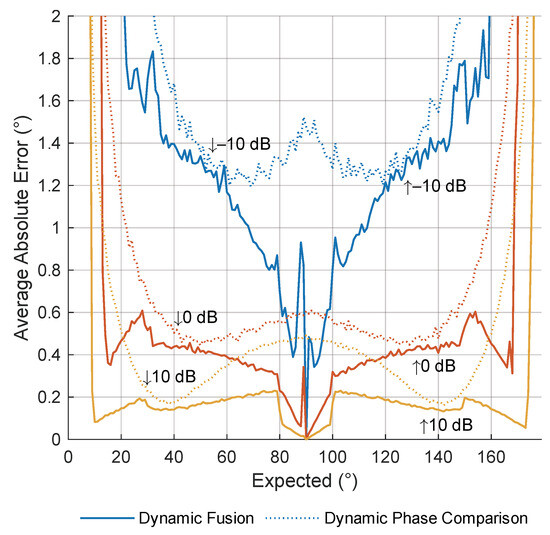
Figure 10.
Average absolute error of the dynamic fusion method and the dynamic phase comparison algorithm under different SNRs.

Table 1.
Analysis of DF accuracy improvement rate.
The simulation results demonstrate that by incorporating the traditional amplitude comparison algorithm, the DF accuracy can be effectively improved under various SNRs with an approximate improvement rate of 6%.
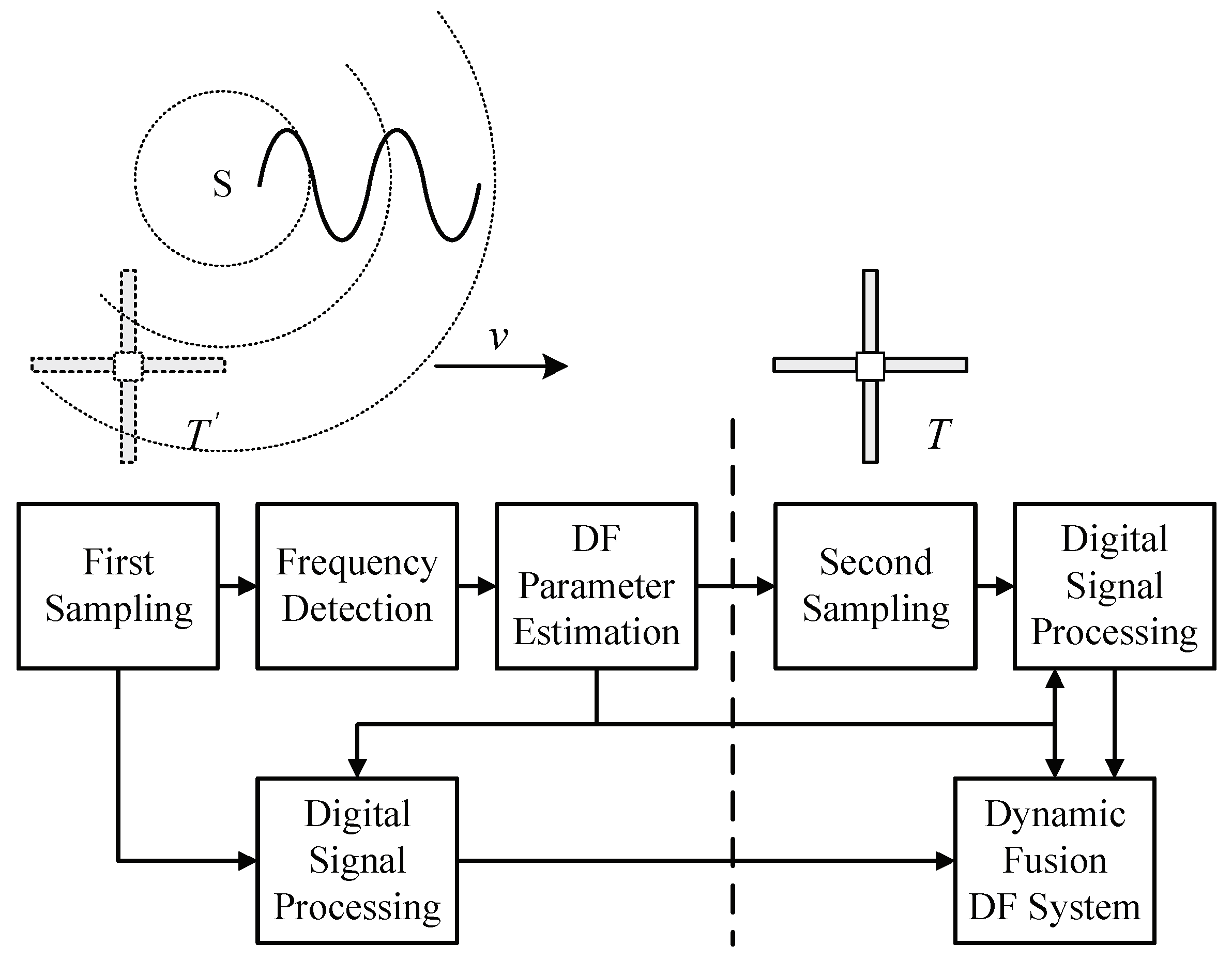
In the DF system of a satellite radio receiver, digital signal processing techniques including band-pass filtering and coherent accumulation can be further introduced to improve the SNR. Figure 11 illustrates the dynamic fusion DF process of the high-speed satellite radio receiver.
Figure 11.
Block diagram of direction-finding system in space-borne receiver.
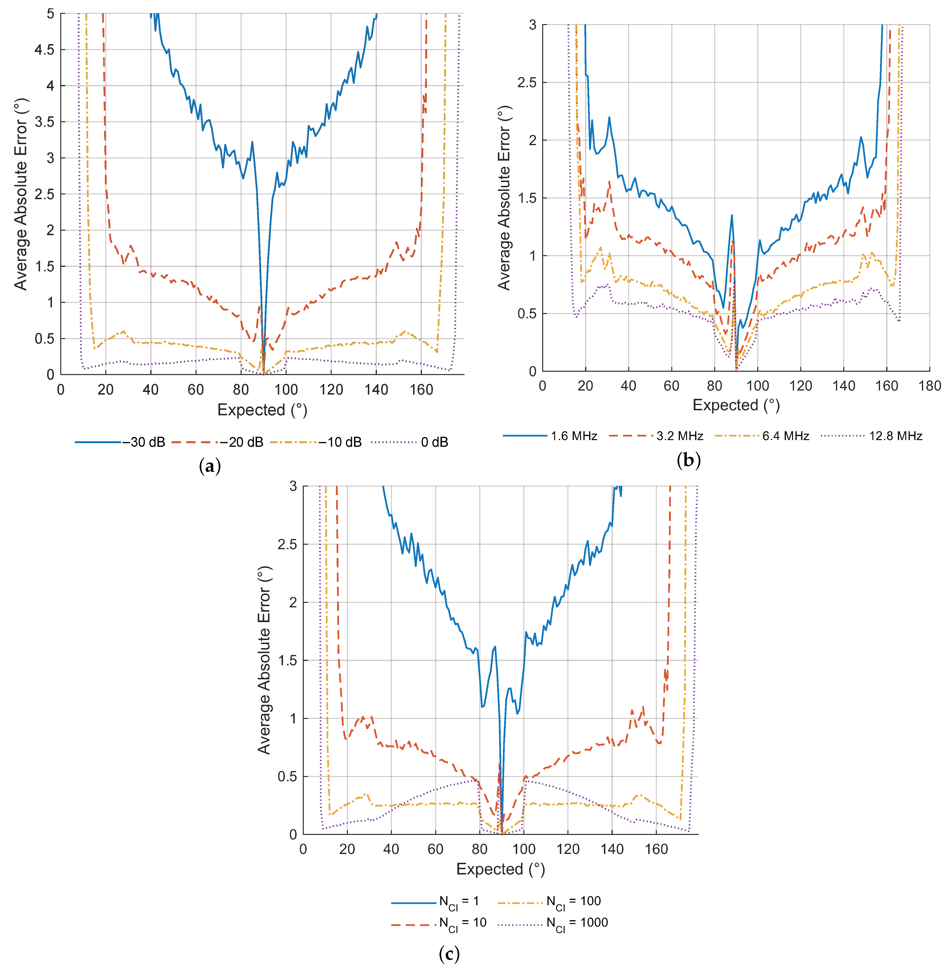
To explore the influence of the SNR, receiver sampling rate, and coherent accumulation on the dynamic fusion DF method, Figure 12 shows the average absolute error curves from one thousand simulations of the dynamic fusion DF method, affected by three factors: SNR, receiver sampling rate, and the number of coherent accumulation. In the simulations, the default parameter settings are as follows: an SNR of −15 dB, a receiver sampling rate of 6.4 MHz, and the number of coherent accumulation set to 10.
Figure 12.
Average absolute error of the dynamic fusion algorithm under different (a) SNRs, (b) receiver sampling rates, (c) and the numbers of coherent accumulation.
The simulation results shows that the SNR, receiver sampling rate, and coherent accumulation all significantly impact the dynamic fusion DF method. When analyzing the simulation results, conclusions slightly different than those in Section 3.1 can be drawn:
- Generally, the higher the SNR, the higher the sampling rate, or the greater the number of coherent accumulation, the higher is the DF accuracy;
- Azimuth angles of EM waves near 0° and 180° may still produce relatively larger DF errors, while errors near 90° become lower, indicating a broader range of DF angles overall;
- The number of coherent accumulation should not also be too large as it may lead to a decrease in DF accuracy. Especially as angles approach 70° or 110°, excessive coherent accumulation number can result in larger errors.
4. Discussion
The simulation analysis from the previous section indicates that the dynamic phase comparison algorithm, when applied to a high-speed moving satellite platform for the direction finding of radiation sources, shows that different target directions significantly affect the direction-finding accuracy. Moreover, as the amplitude comparison algorithm presents a different error curve, integrating both algorithms has led to a new direction-finding method. Planar direction-finding simulation results demonstrate that this method retains a broader direction-finding range while achieving higher accuracy. Additionally, simulations were conducted to analyze the impact of three important factors in the dual orthogonal dipole antenna direction-finding system, which include the SNR, receiver sampling frequency, and coherent accumulation. Given that the spatial amplitude comparison algorithm is typically used in tri-orthogonal dipole antenna systems for direction finding, further research will continue on the performance of the dynamic phase comparison algorithm in the three-dimensional direction finding system.
5. Conclusions
This paper proposes a dynamic phase comparison algorithm for the planar direction finding of radiation sources on a high-speed moving satellite radio receiver. Based on the phase interferometer algorithm, this algorithm treats the high-speed moving antenna as equivalent to single-baseline array antennas. According to the electromagnetic wave frequency and satellite’s velocity, it can adjust the baseline length to avoid phase ambiguity indirectly. Furthermore, compared with the amplitude comparison algorithm used by dual channel receivers, it offers a larger direction-finding range. Finally, by integrating both algorithms, the simulations demonstrate improved accuracy, showing an approximate 6% improvement over the dynamic phase comparison algorithm.
Author Contributions
Conceptualization, Z.W. and K.Y.; methodology, Z.W. and M.M.; software, Z.W. and J.X.; validation, J.X. and Z.Z.; formal analysis, Z.W. and M.M.; investigation, Z.W.; resources, Z.W.; data curation, M.M. and J.X.; writing—original draft preparation, Z.W.; writing—review and editing, M.M., J.X., Z.Z. and K.Y.; visualization, Z.W.; supervision, Z.Z. and K.Y.; project administration, Z.W. and K.Y.; funding acquisition, Z.Z. and K.Y. All authors have read and agreed to the published version of the manuscript.
Funding
This research was supported in part by the Natural Science Foundation of Jiangxi under Grant 20224BAB212027, in part by the Financial Contract of Science and Technology Project of Jiangxi Province under Grant ZBG20230418032, and in part by the Interdisciplinary Innovation Fund of Natural Science from Nanchang University under Grant 9167-28220007-YB2104.
Institutional Review Board Statement
Not applicable.
Informed Consent Statement
Not applicable.
Data Availability Statement
The raw data and source codes supporting the conclusions of this article will be made available by the authors on GitHub https://github.com/wzz91225/DF_Simulations_of_Letter (accessed on 11 April 2024).
Conflicts of Interest
The authors declare no conflicts of interest.
Abbreviations
The following abbreviations are used in this manuscript:
| RPI | Radio plasma imager |
| EM Waves | Electromagnetic waves |
| VLF | Very-low frequency |
| VHF | Very-high frequency |
| DF | Direction finding |
| DOA | Direction of arrival |
| SNR | Signal-to-noise ratio |
References
- Gussenhoven, M.; Mullen, E.; Brautigam, D. Improved understanding of the Earth’s radiation belts from the CRRES satellite. IEEE Trans. Nucl. Sci. 1996, 43, 353–368. [Google Scholar] [CrossRef]
- Reinisch, B.W.; Haines, D.; Bibl, K.; Cheney, G.; Galkin, I.; Huang, X.; Myers, S.; Sales, G.; Benson, R.; Fung, S.; et al. The Radio Plasma Imager investigation on the IMAGE spacecraft. In The IMAGE Mission; Springer: Dordrecht, The Netherlands, 2000; pp. 319–359. [Google Scholar]
- Scherbarth, M.; Smith, D.; Adler, A.; Stuart, J.; Ginet, G. AFRL’s Demonstration and Science Experiments (DSX) mission. In Proceedings of the Solar Physics and Space Weather Instrumentation III, San Diego, CA, USA, 2–6 August 2009; SPIE: Bellingham, WA, USA, 2009; Volume 7438, pp. 101–110. [Google Scholar]
- Kasahara, Y.; Kasaba, Y.; Kojima, H.; Yagitani, S.; Ishisaka, K.; Kumamoto, A.; Tsuchiya, F.; Ozaki, M.; Matsuda, S.; Imachi, T.; et al. The plasma wave experiment (PWE) on board the Arase (ERG) satellite. Earth Planets Space 2018, 70, 1–28. [Google Scholar] [CrossRef]
- Shen, X.; Zhang, X.; Yuan, S.; Wang, L.; Cao, J.; Huang, J.; Zhu, X.; Piergiorgio, P.; Dai, J. The state-of-the-art of the China Seismo-Electromagnetic Satellite mission. Sci. China Technol. Sci. 2018, 61, 634–642. [Google Scholar] [CrossRef]
- Kasaba, Y.; Kojima, H.; Moncuquet, M.; Wahlund, J.E.; Yagitani, S.; Sahraoui, F.; Henri, P.; Karlsson, T.; Kasahara, Y.; Kumamoto, A.; et al. Plasma wave investigation (PWI) aboard BepiColombo Mio on the trip to the first measurement of electric fields, electromagnetic waves, and radio waves around Mercury. Space Sci. Rev. 2020, 216, 65. [Google Scholar] [CrossRef]
- Marshall, R.A.; Sousa, A.; Reid, R.; Wilson, G.; Starks, M.; Ramos, D.; Ballenthin, J.; Quigley, S.; Kay, R.; Patton, J.; et al. The micro-broadband receiver (μBBR) on the very-low-frequency propagation mapper CubeSat. Earth Space Sci. 2021, 8, e2021EA001951. [Google Scholar] [CrossRef]
- Chenglin, D.; Yu, Z.; Yi, H.; Jianfeng, D. Analysis of delay error correction of solar plasma region on Tianwen-1. J. Deep. Space Explor. 2021, 8, 592–599. [Google Scholar]
- Hua, Z.; Bin, Z. Martian space environment magnetic field research: Development and application of the YH-1 precision magnetometer. Physics 2009, 38, 785–792. [Google Scholar]
- Reinisch, B.W.; Sales, G.S.; Haines, D.M.; Fung, S.F.; Taylor, W.W. Radio wave active Doppler imaging of space plasma structures: Arrival angle, wave polarization, and Faraday rotation measurements with the radio plasma imager. Radio Sci. 1999, 34, 1513–1524. [Google Scholar] [CrossRef]
- Xiong, X.; Chunhua, J.; Guobin, Y.; Zhengyu, Z. Simulation study on echo of earth plasma layer detector. J. Deep. Space Explor. 2022, 9, 230–236. [Google Scholar]
- Burke, B.F.; Graham-Smith, F.; Wilkinson, P.N. An Introduction to Radio Astronomy; Cambridge University Press: Cambridge, UK, 2019. [Google Scholar]
- Davies, K. Ionospheric Radio Propagation; US Department of Commerce, National Bureau of Standards: Washington, DC, USA, 1965; Volume 80. [Google Scholar]
- Eckersley, T.L.; Farmer, F. Short period fluctuations in the characteristics of wireless echoes from the ionosphere. Proc. R. Soc. Lond. Ser. A Math. Phys. Sci. 1945, 184, 196–217. [Google Scholar]
- Bramley, E.; Ross, W. Measurements of the direction of arrival of short radio waves reflected at the ionosphere. Proc. R. Soc. Lond. Ser. Math. Phys. Sci. 1951, 207, 251–267. [Google Scholar]
- Ross, W.; Bramley, E.; Ashwell, G. A phase-comparison method of measuring the direction of arrival of ionospheric radio waves. Proc. IEE-Part III: Radio Commun. Eng. 1951, 98, 294–302. [Google Scholar]
- McLeish, C.; Burtnyk, N. The application of the interferometer to hf direction-finding. Proc. IEE-Part B Electron. Commun. Eng. 1961, 108, 495–499. [Google Scholar] [CrossRef]
- Jacobs, E.; Ralston, E.W. Ambiguity resolution in interferometry. IEEE Trans. Aerosp. Electron. Syst. 1981, 6, 766–780. [Google Scholar] [CrossRef]
- Lee, J.H.; Woo, J.M. Interferometer direction-finding system with improved DF accuracy using two different array configurations. IEEE Antennas Wirel. Propag. Lett. 2014, 14, 719–722. [Google Scholar] [CrossRef]
- Liu, Z.M.; Guo, F.C. Azimuth and elevation estimation with rotating long-baseline interferometers. IEEE Trans. Signal Process. 2015, 63, 2405–2419. [Google Scholar] [CrossRef]
- Van Doan, S.; Vesely, J.; Janu, P.; Hubacek, P.; Tran, X.L. Algorithm for obtaining high accurate phase interferometer. In Proceedings of the 2016 26th International Conference Radioelektronika (RADIOELEKTRONIKA), Kosice, Slovakia, 19–20 April 2016; IEEE: Piscataway, NJ, USA, 2016; pp. 433–437. [Google Scholar]
- He, C.; Chen, J.; Liang, X.; Geng, J.; Zhu, W.; Jin, R. High-accuracy DOA estimation based on time-modulated array with long and short baselines. IEEE Antennas Wirel. Propag. Lett. 2018, 17, 1391–1395. [Google Scholar] [CrossRef]
- Liu, L.; Yu, T. An analysis method for solving ambiguity in direction finding with phase interferometers. Circuits Syst. Signal Process. 2021, 40, 1420–1437. [Google Scholar] [CrossRef]
- Kawase, S. Radio interferometer for geosynchronous-satellite direction finding. IEEE Trans. Aerosp. Electron. Syst. 2007, 43, 443–449. [Google Scholar] [CrossRef]
- Li, T.; Guo, F.; Jiang, W. A novel emitter localization method using an interferometer on a spin-stabilized satellite. In Proceedings of the 2010 International Conference on Wireless Communications & Signal Processing (WCSP), Suzhou, China, 21–23 October 2010; IEEE: Piscataway, NJ, USA, 2010; pp. 1–5. [Google Scholar]


Disclaimer/Publisher’s Note: The statements, opinions and data contained in all publications are solely those of the individual author(s) and contributor(s) and not of MDPI and/or the editor(s). MDPI and/or the editor(s) disclaim responsibility for any injury to people or property resulting from any ideas, methods, instructions or products referred to in the content. |
© 2024 by the authors. Licensee MDPI, Basel, Switzerland. This article is an open access article distributed under the terms and conditions of the Creative Commons Attribution (CC BY) license (https://creativecommons.org/licenses/by/4.0/).