Output Feedback Tracking Control for Vessel with Collision-Avoidance and Performance Constraints

Abstract

This manuscript investigates an output feedback-tracking control problem of a dynamically positioned vessel with an input constraint. The vessel is exposed to model uncertainty and external disturbances. Compared with the existing results, the primary contribution is to develop a switch-control strategy for achieving collision avoidance and performance constraints by using an extended state observer (ESO), a collision-avoidance controller (CAC), a prescribed performance controller, and an auxiliary dynamic system (ADS). The switch control strategy combined two different controllers, and an extended state observer (ESO) is designed. The ESO is employed to recover velocity information as well as unknown model uncertainty and external disturbances. A collision-risk-analysis module is introduced to evaluate whether there exists a risk of collision avoidance. Based on the analysis, the CASC can choose between a CAC and a PPC. An ADS is constructed to handle the input constraints. The CAC is employed by using an artificial potential function, the ADS, and the ESO. The PPC is designed based on an error constraint function, the ADS, and the ESO. The stability of the closed-loop control system is analyzed based on the Lyapunov direct method. Simulations prove the effectiveness of the presented control strategy.

1. Introduction

An automatic ship motion controller can automatically achieve positioning or trajectory-tracking operations by using its own thrusters, propellers, and rudders [1,2,3,4], and trajectory-tracking control is widely used in engineering [5,6,7]. With the development of deep-sea exploration activities, there are higher requirements for the vessel. The vessel that is working at sea inevitably suffers from environmental disturbances [8], and its mathematical model contains model uncertainty. In addition, the control inputs are constrained due to the physical limitations of the vessel’s propulsion system [9]. Furthermore, in an area with busy sea traffic, vessels inevitably come across various obstacles, and crashes may occur when achieving a desired trajectory. To ensure high performance and safe maneuvering, disturbances, input constraints, and collision avoidance should be considered in dynamic position-control design.

To deal with model uncertainty and external disturbances, passive and active approaches are both designed for vessels. The active approach incorporates an adaptive observer-exploit estimation of the unknown item to indemnify these effects, and the passive approaches depend on the designed controller’s robustness [10,11,12,13]. To ensure control performance and decrease the difficulty of controller design, the active approach is usually preferred to the passive approaches. A global robust controller combined with an adaptive observer is superior when solving the dynamic positioning control of surface vessels [14]. The observer is based on velocity measurements, which can not only increase the cost of the system but also restrict the range of applications. To avoid this, an observer is employed to approximate velocity and disturbances in [15,16]. Nevertheless, the observer requires prior knowledge of disturbances. To avoid this problem, an extended state observer (ESO) is developed for a dynamically positioned vessel in [17]. The observer can estimate velocities, model uncertainty, and external disturbances without using velocity measurements.

In practice, owing to physical limitations, control inputs are limited by magnitude constraints. The saturated control inputs may impact the system performance [18]. To ensure a stable and efficient work system, many methods have been widely explored for vessels. Considering input constraints, a controller combined with a Gaussian function is proposed for dynamically positioned vessels [19], and the Gaussian function is designed to approximate input saturation induced by physical limitations of thrusters. A hyperbolic tangent function is employed to solve the input saturation in [20]. However, those functions limit control inputs and degrade system performance, whether the control inputs are saturated or not. To avoid this, ref. [21] proposes a robust control scheme for dynamically positioned vessels, and an auxiliary dynamic system (ADS) is used to solve input constraints. An anti-windup compensator is combined with a control design to solve the input saturation in the trajectory tracking of a dynamically positioned vessel [22,23].

Most of the aforementioned results do not consider prescribed performance in the control design. In a complex sea environment, collisions may occur due to a larger tracking error. Ref. [24] proposes a logarithmic error mapping function to realize the prescribed control performance, and it is widely used in nonlinear systems. Furthermore, ref. [25] designs control laws with prescribed performance for nonlinear systems with strict feedback. Ref. [26] proposes the prescribed performance control for dynamically positioned vessels, where a finite-time controller combined with a nonlinear observer is constructed.

Apart from the prescribed performance, the collision avoidance must be considered. An efficient collision-avoidance algorithm can enhance navigation safety. Using a path planning algorithm is one of the most popular methods [27]. The method is limited by optimization strategies; it takes a lot of time to obtain an available solution. The existing path-planning algorithms have not been able to effectively deal with complex traffic environments, and it is sometimes impossible to obtain a feasible solution within a feasible time. To solve this, some researchers have designed collision-avoidance control systems for vessels [28,29]. Ref. [30] introduces a collision-avoidance function for a recursive control design, in which dynamic obstacles can be avoided through the control design. However, input constraints are neglected in the controller design process, which has a great impact on the collision-avoidance ability. To get around this, Ref. [31] proposes a new control strategy combined with modified artificial potential functions for dynamically positioned vessels with input saturation.

In view of the experience of navigation practice, the capabilities of collision avoidance have a great impact on the safety of navigation. On one hand, the capabilities of collision avoidance are limited to the performance of the actuator, and balancing the avoidance collision ability and the limited performance of the actuator is a challenging subject. On the other hand, the performance of the control system is closely related to navigation security. Poor performance of the control system leads to great tracking errors, and collisions may occur during transportation, especially during narrow waters.

As far as is known, no results have been reported on vessels with collision avoidance in the simultaneous presence of input constraints and prescribed performance. This paper aims to propose a collision avoidance switch control (CASC) strategy for vessels. A dynamic calculation of collision risk (DCCR) is introduced to evaluate whether there exists a risk of collision avoidance. Based on the analysis of the DCCR, the DCCR can choose between a collision-avoidance controller (CAC) and a prescribed performance controller (PPC). Then, an ADS is constructed to handle the input constraints. The collision-avoidance controller (CAC) is designed based on an artificial potential function, the ADS, and the ESO. The prescribed performance controller (PPC) is designed based on an error constraint function, the ADS, and the ESO. The system’s stability is proved based on the Lyapunov direct method. Simulation outcomes verify the effectiveness of the presented control strategy. The main contributions are summarized as follows.

(1) Compared with the existing related results [21,22,24], input saturation and collision avoidance are considered simultaneously in the controller design.

(2) In contrast to the control approach proposed in [31], the CASC introduces a dynamic calculation of collision risk, which is used for generating decisions between the CAC and PPC. The CASC is valid with a faster simulation rate and less error, regardless of the trajectory tracking or collision avoidance.

The remaining sections are as follows. Section 2 gives the problem formulated. Section 3 gives an observer design. Section 4 presents the collision-avoidance switch control strategy. The simulation is designed in Section 5. Conclusions are given in Section 6.

2. Problem Formulation

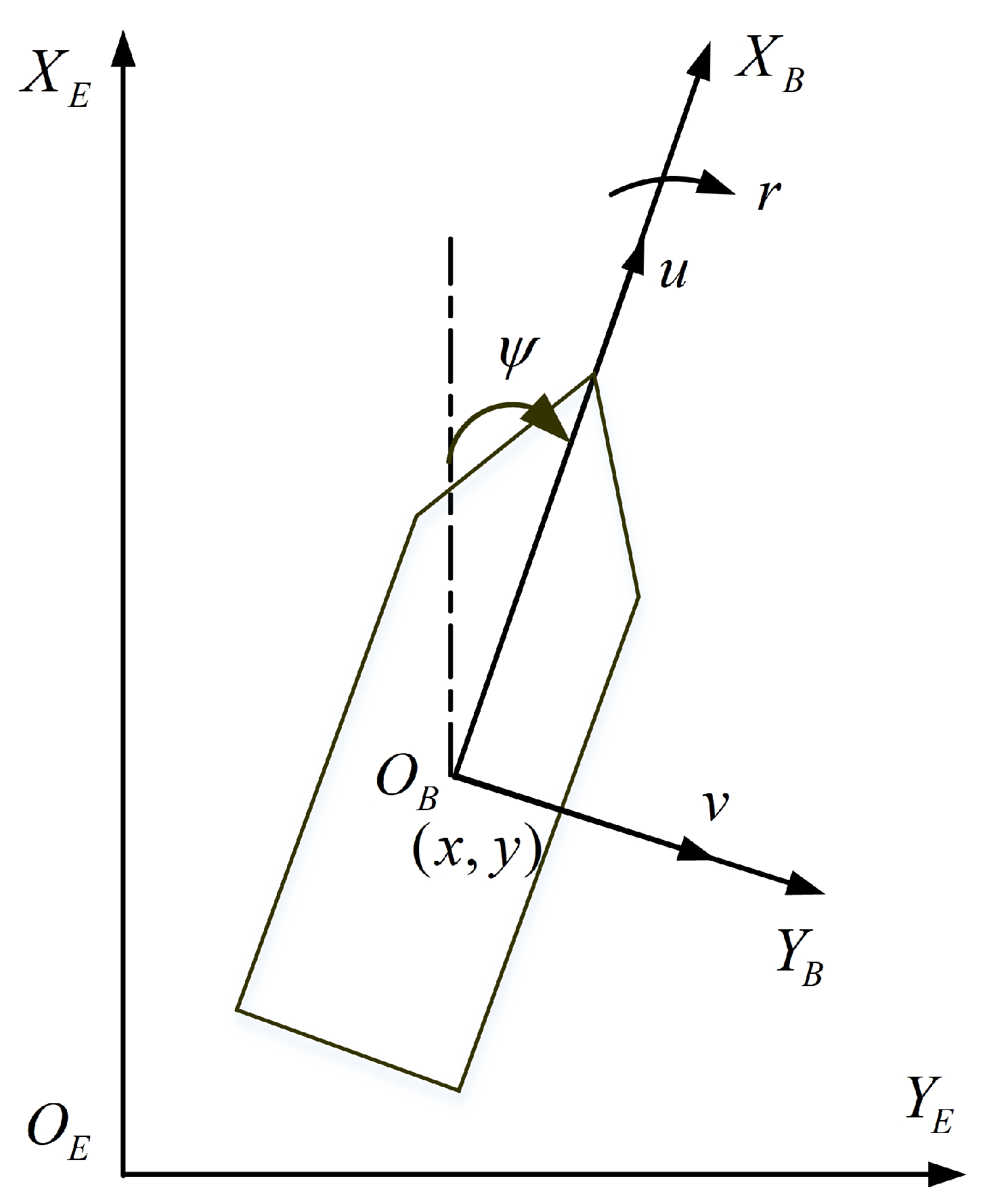
As shown in Figure 1, the vessel’s mathematical model is

$$\begin{array}{cc}\hfill \dot{\eta }=& R\left(\psi \right)\nu \hfill \end{array}$$

(1)

$$\begin{array}{cc}\hfill M\dot{\nu }+C\nu +D\nu =& \tau +d,\hfill \end{array}$$

(2)

where $\eta ={[x,y,\psi ]}^{\mathrm{T}}$ is the vector containing position $(x,y)$ and yaw angle $\psi$, which is expressed in earth-fixed frame $X_E{O}_E{Y}_E$. $\nu ={[u,v,r]}^{\mathrm{T}}$ is the velocity vector expressed in the body-fixed frame $X_B{O}_B{Y}_B$, u and v are surge and sway, and r is the yaw velocity. $M\in {\mathbb{R}}^{3\times 3}$ is the positive definite inertia matrix including added mass. $C\in {\mathbb{R}}^{3\times 3}$ is the skew-symmetric matrix of Coriolis and the centripetal term. $D\in {\mathbb{R}}^{3\times 3}$ is the positive definite damping matrix. $\tau ={[{\tau }_u,{\tau }_v,{\tau }_r]}^{\mathrm{T}}$ is the input signal of the vessel control system, which is generated using the thruster system. d values are the external environmental disturbances. R denotes the rotation matrix, defined as

$$R\left(\psi \right)=\left[\begin{array}{ccc}\cos \left(\psi \right)& -\sin \left(\psi \right)& 0\\ \sin \left(\psi \right)& \cos \left(\psi \right)& 0\\ 0& 0& 1\end{array}\right].$$

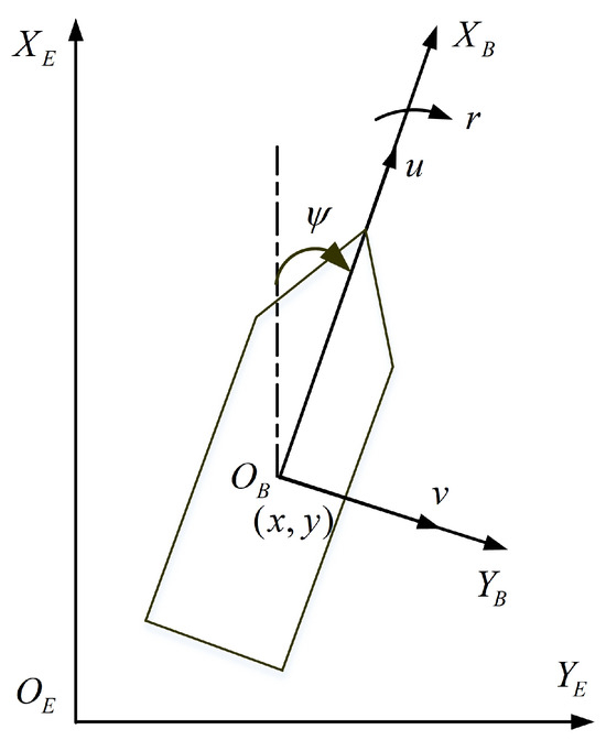
Figure 1. Earth-fixed frame and body-fixed frame.

In practice, owing to the thruster system’s physical limitations, control inputs are limited. And the input limitation is modeled as

$$\tau =\left\{\begin{array}{ccc}\hfill {\tau }_{max}& & {\tau }_c>{\tau }_{max}\hfill \\ \hfill {\tau }_c& & {\tau }_{min}\le {\tau }_c\le {\tau }_{max}\hfill \\ \hfill {\tau }_{min}& & {\tau }_c<{\tau }_{min}\hfill \end{array}\right.$$

where ${\tau }_{max}$ denotes the maximum constraint of control force and moment, ${\tau }_{min}\in {\mathbb{R}}^3$ denotes the maximum constraint of the minimum control force and moment, a mismatch function is used to describe the impact of input saturation defined as $\varpi ={\tau }_c-\tau$, ${\tau }_c={[{\tau }_{uc},{\tau }_{vc},{\tau }_{rc}]}^{\mathrm{T}}$ is the control force, and moment is calculated using the proposed controller.

The control objective is given as follows:

$$\begin{array}{c}\hfill \underset{t\to +\infty }{lim}\parallel \eta -{\eta }_d\parallel <c_1\end{array}$$

(3)

where ${\eta }_d$ denotes the desired trajectory, $c_1$ denotes a tracking error, and it is a small positive constant.

Assumption 1.

The desired trajectory ${\eta }_d$ and derivative ${\dot{\eta }}_d$ are bounded.

Remark 1.

Assumption 1 means that the desired trajectory is sufficiently smooth so that the dynamically positioned vessel can successfully track it. And the desired position-heading of the desired trajectory is available.

3. Observer Design

To provide the estimations of velocity vector $\nu$ and the unknown term $\zeta =M^{-1}(-C\nu -D\nu +d)$, the dynamically positioned vessel model (1) and (2) is rewritten as

$$\begin{array}{cc}\hfill \dot{\eta }=& R\left(\psi \right)\nu \hfill \end{array}$$

(4)

$$\begin{array}{cc}\hfill \dot{\nu }=& M^{-1}\tau +\zeta .\hfill \end{array}$$

(5)

Assumption 2.

$\parallel \dot{\zeta }\parallel \le {\zeta }^{*}$, and ${\zeta }^{*}$ is a positive constant.

To provide the estimations of the unknown term $\zeta$, we define an ESO as follows:

$$\begin{array}{cc}\hfill \dot{\widehat{\eta }}=& -K_{o1}\tilde{\eta }+R\left(\psi \right)\widehat{\nu },\hfill \end{array}$$

(6)

$$\begin{array}{cc}\hfill \dot{\widehat{\nu }}=& -K_{o2}{R}^{\mathrm{T}}\left(\psi \right)\tilde{\eta }+\widehat{\zeta }+M^{-1}\tau ,\hfill \end{array}$$

(7)

$$\begin{array}{cc}\hfill \dot{\widehat{\zeta }}=& -K_{o3}{R}^{\mathrm{T}}\left(\psi \right)\tilde{\eta }\hfill \end{array}$$

(8)

where $\tilde{\eta }=\widehat{\eta }-\eta$ is the position-heading estimation error, and $\widehat{\eta }={[\widehat{x},\widehat{y},\widehat{\psi }]}^{\mathrm{T}}\in {\mathbb{R}}^3$, $\widehat{\nu }={[\widehat{u},\widehat{v},\widehat{r}]}^{\mathrm{T}}\in {\mathbb{R}}^3$, $\widehat{\zeta }={[{\widehat{\zeta }}_1,{\widehat{\zeta }}_2,{\widehat{\zeta }}_3]}^{\mathrm{T}}\in {\mathbb{R}}^3$, $\widehat{x}$, $\widehat{y}$, $\widehat{\psi }$, $\widehat{u}$, $\widehat{v}$, $\widehat{r}$, ${\widehat{\zeta }}_1$, ${\widehat{\zeta }}_2$, ${\widehat{\zeta }}_3$ are the estimates of x, y, $\psi$, u, v, r, ${\zeta }_1$, ${\zeta }_2$ and ${\zeta }_3$. $K_{o1}\in {\mathbb{R}}^{3\times 3}$, $K_{o2}\in {\mathbb{R}}^{3\times 3}$ and $K_{o3}\in {\mathbb{R}}^{3\times 3}$ are gain matrices.

From (4)–(8), the estimation errors can be given as

$$\begin{array}{cc}\hfill \dot{\tilde{\eta }}& =-K_{o1}\tilde{\eta }+R\left(\psi \right)\tilde{\nu },\hfill \\ \hfill \dot{\tilde{\nu }}& =-K_{o2}{R}^T\left(\psi \right)\tilde{\eta }+\tilde{\zeta },\hfill \\ \hfill \dot{\tilde{\zeta }}& =-K_{o3}{R}^T\left(\psi \right)\tilde{\eta }-\dot{\zeta },\hfill \end{array}$$

(9)

where error, $\tilde{\nu }=\widehat{\nu }-\nu$ is the velocity estimation error, and $\tilde{\zeta }=\widehat{\zeta }-\zeta$ is the unknown term’s estimation error.

To make the analyses convenient, the observer error dynamics (9) are given as

$$\begin{array}{cc}\hfill \dot{X}=& AX+B\varphi \hfill \end{array}$$

(10)

$$\begin{array}{cc}\hfill \tilde{\eta }=& C_{o}X,\hfill \end{array}$$

(11)

where $X={[{\tilde{\eta }}^T,{\tilde{\nu }}^T,{\tilde{\zeta }}^T]}^T\in {\mathbb{R}}^{9\times 1}$,

$$A=\left[\begin{array}{ccc}-K_{o1}& R\left(\psi \right)& 0_3\\ -K_{o2}{R}^T\left(\psi \right)& 0_3& I_3\\ -K_{o3}{R}^T\left(\psi \right)& 0_3& 0_3\end{array}\right],$$

(12)

$$B=\left[\begin{array}{c}{0}_3\\ 0_3\\ I_3\end{array}\right],$$

(13)

$$C_{oi}=\left[\begin{array}{ccc}{I}_3& 0_3& 0_3\end{array}\right],$$

(14)

and $\varphi =-\dot{\zeta }$. $0_3$ represents a $3\times 3$ dimensional zero matrix. $I_3$ represents a $3\times 3$ dimensional identity matrix.

To make the stability analysis of the ESO convenient, a transformation $\chi =TX$ with $T=\mathrm{diag}\{R^T\left(\psi \right)$, $I_3,I_3\}$ is introduced to remove the nonlinear term $R\left(\psi \right)$. We have

$$\begin{array}{c}\hfill \dot{\chi }=(A_0+r{S}_T)\chi +B\varphi ,\end{array}$$

(15)

where $S_T=\mathrm{diag}\{S_1,0_3,0_3\}$, $\overline{\varphi }$ denotes a positive constant, and we make the assumption that $\parallel \varphi \parallel \le \overline{\varphi }$ according to Assumption 2.

$$S_1=\left[\begin{array}{ccc}0& 1& 0\\ -1& 0& 0\\ 0& 0& 0\end{array}\right],$$

(16)

$$A_0=\left[\begin{array}{ccc}-K_{o1}& I_3& 0_3\\ -K_{o2}& 0_3& I_3\\ -K_{o3}& 0_3& 0_3\end{array}\right].$$

(17)

Lemma 1.

The estimation error X is bounded; if there are symmetric definite positive matrices $Q,P\in {\mathbb{R}}^{9\times 9}$ results in

$$\begin{array}{cc}\hfill A_0^{T}P& +P{A}_0+PB{B}^{T}P+Q\hfill \\ \hfill & +\overline{r}(S_T^{T}P+P{S}_T)\le 0,\hfill \end{array}$$

(18)

$$\begin{array}{cc}\hfill A_0^{T}P& + P{A}_0+PB{B}^{T}P+Q\hfill \\ \hfill & -\overline{r}(S_T^{T}P+P{S}_T)\le 0,\hfill \end{array}$$

(19)

$\overline{r}\in \mathbb{R}$ is the upper bound of r.

Proof. 

Chose a Lyapunov function as follows

$$\begin{array}{c}\hfill V_o=\frac{1}{2}{\chi }^{T}P\chi .\end{array}$$

(20)

Differentiating $V_o$ with respect to time,

$$\begin{array}{cc}\hfill V_o=& \frac{1}{2}{\chi }^T(P{A}_0+A_0^{T}P+rP{S}_T+r{S}_T^{T}P)\chi +{\chi }^{T}PB\varphi \hfill \\ \hfill \le & \frac{1}{2}{\chi }^T(P{A}_0+A_0^{T}P+rP{S}_T+r{S}_T^{T}P+PB{B}^{T}P)\chi +\frac{1}{2}{\varphi }^T\varphi \hfill \\ \hfill & \le -c_{o_1}{V}_o+c_{o_2},\hfill \end{array}$$

(21)

where $c_{o_1}=\frac{{\lambda }_{min}\left(Q\right)}{{\lambda }_{max}\left(P\right)}$, $c_{o_2}=\frac{1}{2}{\overline{\varphi }}^2$. Since $c_{o_2}$ is symmetric definite positive, the state ${\chi }_i$ is bounded using $\parallel T^{-1}\parallel =1$ and $X=T^{-1}\chi$. The estimation error signal X is bounded. □

4. Collision-Avoidance Switch Control Strategy

This section describes a CASC, and the structure of the CASC is shown in Figure 2. A dynamic calculation of collision risk (DCCR) is introduced to evaluate the risk of collision. Based on the COLREGs, this paper classifies four encountering situations of two vessels: the head-on situation, the left crossing situation, the right crossing situation, and the overtaking situation are considered [32,33]. More details of the encountering situations can be found in rules 13, 14, and 15 of the COLREGs [34,35], which are depicted in Figure 3. Based on the DCCR analysis, a switch control strategy is employed. A collision-avoidance controller (CAC) and a prescribed performance controller are designed, and the stability of the control system is proven.

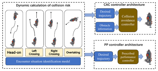
Figure 2. The structure of the collision-avoidance switch control (CASC) strategy.

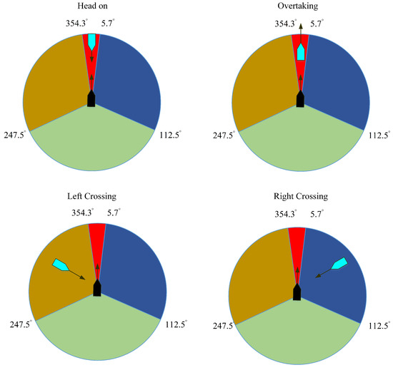
Figure 3. Different vessel encounter situations.

4.1. Dynamic Calculation of Collision Risk

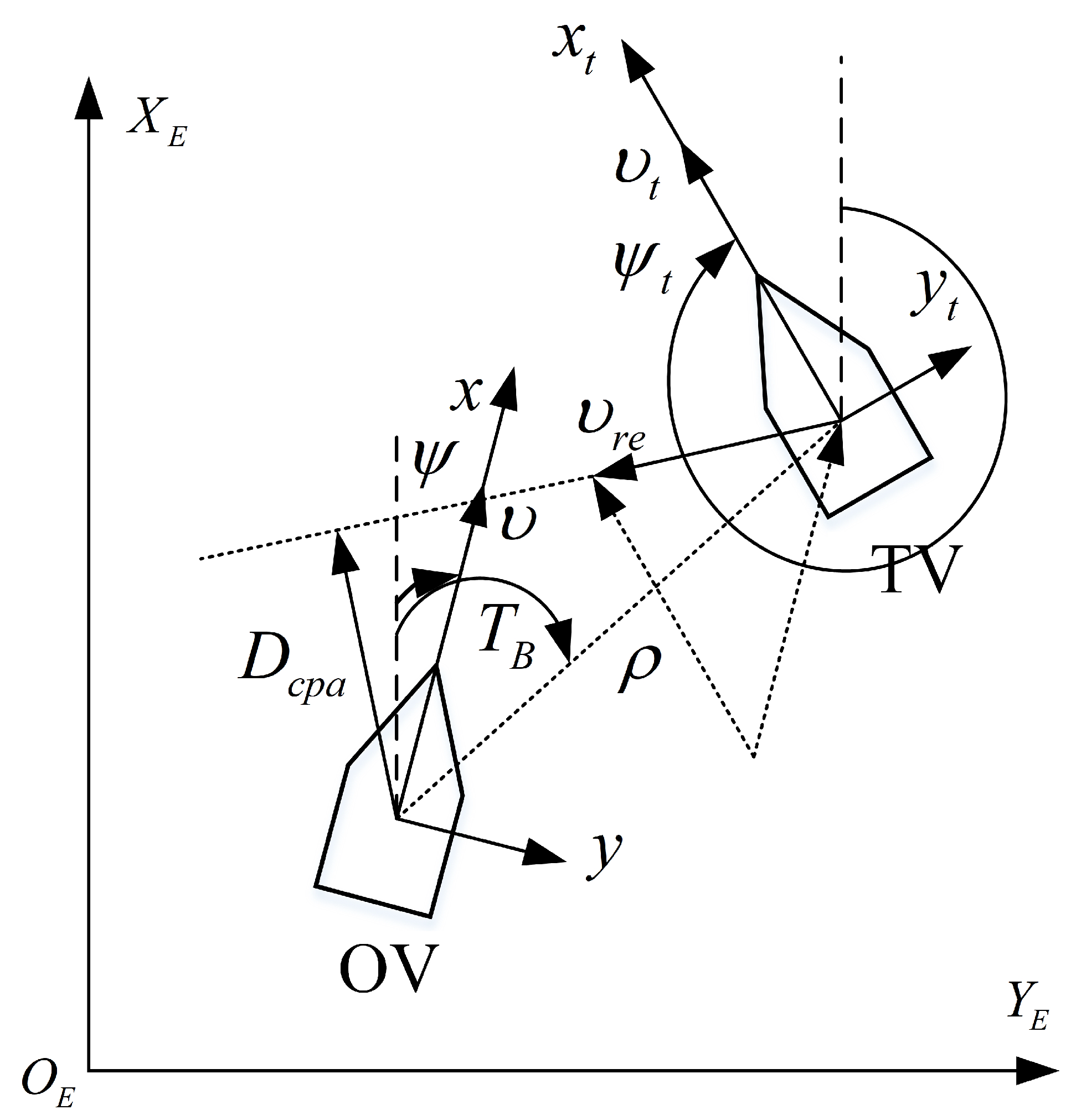
The vessel is defined as its own vessel (OV), and its position and yaw and speed are $(x,y,\psi )$ and $\nu$. Other vessels or obstacles are considered to be the target vessel (VS), and their position and yaw and speed are defined as $(x_t,y_t,{\psi }_t)$ and ${\nu }_t$. $T_B$ is the true bearing of the TV from the OV, and TC is the true course of the OV, which is defined as follows:

$$\begin{array}{c}\hfill T_B=atan2(y_t-y,x_t-x).\end{array}$$

(22)

The relative relationship between OV and TV is given in Figure 4.

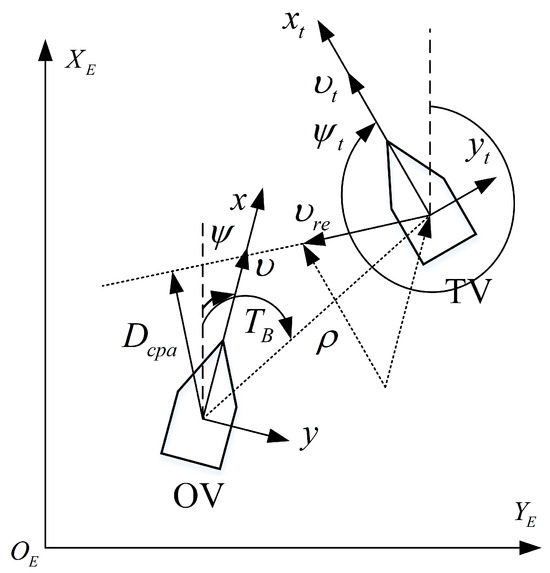
Figure 4. Different encountering situations.

The function of collision risk index $C_{ri}$ is defined as follows:

$$\begin{array}{cc}\hfill C_{ri}& =\{D_{cpa},T_{cpa},\rho ,K,Q\}\hfill \\ \hfill & =[{\alpha }_{Dcpa},{\alpha }_{Tcpa},{\alpha }_D,{\alpha }_K,{\alpha }_Q]\times [u_{dcpa},u_{tcpa},u_D,u_K,u_D],\hfill \end{array}$$

(23)

where $D_{cpa}$ is the closest point of the approach, $T_{cpa}$ is the time to the closest point of the approach, $Q=T_B-\psi$ is the true bearing, and K is the speed ratio between the two vessels. $\rho$ is the distance, defined as

$$\begin{array}{c}\hfill \rho =\sqrt{{(x_t-x)}^2+{(y_t-y)}^2}\end{array}$$

(24)

Next, the functions $D_{cpa},T_{cpa},K$, and Q will be introduced one by one.

(1) The membership function of $D_{cpa}$ is as follows:

$$\begin{array}{c}\hfill \begin{array}{cc}\hfill u_{dcpa}=& \left\{\begin{array}{cc}1,\hfill & D_{cpa}\le d_1,\hfill \\ \{1-sin\left[\frac{\pi }{d_2-d_1}(D_{cpa}-\frac{d_2+d_1}{2})\right]\}/2,\hfill & d_1<D_{cpa}<d_2,\hfill \\ 0,\hfill & d_2<D_{cpa},\hfill \end{array}\right.\hfill \end{array}\end{array}$$

(25)

$$\begin{array}{c}\hfill \begin{array}{cc}\hfill d_1=& \left\{\begin{array}{cc}1.1-\frac{Q}{{180}^{\circ }}\times 0.2,\hfill & 0^{\circ }\le Q\le 112.5^{\circ },\hfill \\ \\ 1-\frac{{270}^{\circ }-Q}{{180}^{\circ }}\times 0.8,\hfill & 112.5^{\circ }\le Q\le 247.5^{\circ },\hfill \\ \\ 1.1-\frac{{360}^{\circ }-Q}{{180}^{\circ }}\times 0.4,\hfill & 247.5^{\circ }\le Q\le {360}^{\circ },\hfill \end{array}\right.\hfill \end{array}\end{array}$$

(26)

where $d_1$ represents the smallest safe encounter distance between OV and TV, and $d_2$ denotes the minimum distance between the own ship and the target ship, $d_2=2d_1$.

(2) The membership function of $T_{cpa}$ is as follows:

$$\begin{array}{c}\hfill \begin{array}{cc}\hfill u_{tcpa}=& \left\{\begin{array}{cc}1,\hfill & |T_{cpa}|\le t_1,\hfill \\ \left(\right(t_2-|T_{cpa}\left|\right)/(t_2-t_1){)}^2,\hfill & t_1<\left|T_{cpa}\right|\le t_2,\hfill \\ 0,\hfill & d_2<T_{cpa},\hfill \end{array}\right.\hfill \end{array}\end{array}$$

(27)

where $t_2$ denotes the time that the vessel sails from the current position to the point with the minimum distance, $t_1$ is the time that the vessel sails from the point of evasive actions to the closest point of approach, and $t_1$ and $t_2$ are calculated from the following equations:

$$\begin{array}{c}\hfill \begin{array}{cc}\hfill t_1=& \left\{\begin{array}{cc}\sqrt{(d_1^2-D_{cpa}^2)}/v_{ot},\hfill & |T_{cpa}| \le t_1,\hfill \\ (d_1-D_{cpa})/v_{ot},\hfill & D_{cpa}>d_1\hfill \end{array}\right.\hfill \\ \hfill t_2=& \sqrt{(d_2^2-D_{cpa}^2)}/v_{ot};\hfill \end{array}\end{array}$$

(28)

$v_{ot}$ is the relative speed between the two ships.

(3) The function $u_D$ is given as

$$\begin{array}{c}\hfill \begin{array}{cc}\hfill u_D=& \left\{\begin{array}{cc}1,\hfill & \rho \le d_1,\hfill \\ {(d_2-\rho /d_2-d_1)}^2,\hfill & d_1<\rho <d_2,\hfill \\ 0,\hfill & d_2\le \rho ,\hfill \end{array}\right.\hfill \end{array}\end{array}$$

(29)

(4) The function $u_K$ is given as

$$\begin{array}{c}\hfill u_K=\frac{1}{1+\frac{2}{K\sqrt{K^2+1+2K|sin(|\psi -{\psi }_t\left|\right)|}}}.\end{array}$$

(30)

(5) The function $u_Q$ is given as

$$\begin{array}{c}\hfill u_Q=0.5\ast [cos(Q-{19}^{\circ })+\sqrt{440/289+{cos}^2(Q-{19}^{\circ })}]-5/17,\end{array}$$

(31)

where $0\le Q\le 360$.

The function of collision risk index $C_{ri}$ is formulated as

$$\begin{array}{cc}\hfill C_{ri}& =[{\alpha }_{Dcpa},{\alpha }_{Tcpa},{\alpha }_D,{\alpha }_K,{\alpha }_Q]\times [u_{dcpa},u_{tcpa},u_D,u_K,u_D],\hfill \end{array}$$

(32)

where ${\alpha }_{Dcpa}$, ${\alpha }_{Tcpa}$, ${\alpha }_D$, ${\alpha }_K$ and ${\alpha }_Q$ are weight coefficients, and their value ranges are [0, 1]. The sum of ${\alpha }_{Dcpa}$, ${\alpha }_{Tcpa}$, ${\alpha }_D$, ${\alpha }_K$ and ${\alpha }_Q$ is 1.

4.2. Switching Control Strategy

Based on the analysis of the DCCR, the CASC can choose between a collision-avoidance controller (CAC) and a prescribed performance controller (PPC). A switching control strategy is proposed as follows:

$$\begin{array}{c}\hfill \begin{array}{c}\hfill {\tau }_c=\left\{\begin{array}{cc}{\tau }_{ppc},\hfill & C_{ri}=0,\hfill \\ {\tau }_{cac},\hfill & C_{ri}>0,\hfill \end{array}\right.\end{array}\end{array}$$

(33)

where ${\tau }_{ppc}$ is the control input of the PPC and ${\tau }_{cac}$ is the control input of the CAC.

To achieve the prescribed error constraints and collision avoidance, a novel control strategy, which consists of a prescribed performance controller and a collision-avoidance controller with an anti-windup compensator algorithm based on switching logic, is proposed. The proposed controller is presented step by step.

4.3. Prescribed Performance Controller Design

Step 1: A prescribed error function is defined as

$$\begin{array}{c}\hfill z_1=\frac{1}{2}\mathrm{In}\frac{k_b^2}{k_b^2-{\eta }_e^T{\eta }_e},\end{array}$$

(34)

where $k_b$ is a constraint function that is employed to achieve the required prescribed performance, and it is given as follows:

$$\begin{array}{cc}\hfill k_b\left(t\right)=& {\delta }_l[({\rho }_0-{\rho }_{\infty })e^{-kt}+{\rho }_{\infty }]\hfill \end{array}$$

(35)

where ${\delta }_l$, ${\rho }_0$, ${\rho }_{\infty }$, and k are positive constants and ${\rho }_0$ is satisfied such that ${\rho }_0\ge {\eta }_e{\left(0\right)}^T{\eta }_e\left(0\right)$. ${\rho }_{\infty }$ defines the steady-state value of the performance function. k is the bound of the error-convergence rate. ${\eta }_e=\eta -{\eta }_d$.

The time derivative of $z_1$ is

$$\begin{array}{cc}\hfill {\dot{z}}_1=& \frac{{\eta }_e^T{\dot{\eta }}_e}{k_b^2-{\eta }_e^T{\eta }_e}+\frac{-k_b{\dot{k}}_b}{k_b^2-{\eta }_e^T{\eta }_e}+\frac{{\dot{k}}_b}{k_b}.\hfill \end{array}$$

(36)

To stabilize the error $z_1$, the desired virtual control $\alpha$ is given as:

$$\begin{array}{c}\hfill \alpha =R^T[{\dot{\eta }}_d-K_1{\eta }_e-\frac{k_b^2-{\eta }_e^T{\eta }_e}{1+ϵ\ast \mathrm{sign}\left({\eta }_e\right)}\Delta ],\end{array}$$

(37)

where $K_1\in {\mathbb{R}}^{3\times 3}$ is a positive definite matrix, $ϵ\ne 1$ is a positive constant, and

$$\begin{array}{c}\hfill \Delta =\frac{k_{ib}^T{\dot{k}}_{ib}}{k_{ib}^T{k}_{ib}-z_1^T{z}_1}-\frac{{\dot{k}}_b}{k_b}.\end{array}$$

(38)

Step 2: In this step, a kinetic controller is developed. The velocity error vector is defined as

$$\begin{array}{c}\hfill z_2=\widehat{\nu }-\overline{\alpha }-\beta ,\end{array}$$

(39)

where $\beta$ is the parameter of the ADS. $\overline{\alpha }$ is employed to avoid the computation of $\dot{\alpha }$, a first-order filter $l\dot{\overline{\alpha }}+\overline{\alpha }=\alpha$ is introduced instead of the time derivative of $\alpha$, and l is a positive time constant. The update law of $\beta$ is chosen as

$$\begin{array}{c}\hfill \dot{\beta }=-K_r\beta -K_m\mathrm{sign}\left(\beta \right)-\frac{\frac{1}{2}{\Delta }_{\tau }^T{\Delta }_{\tau }}{{\parallel \beta \parallel }^2}\beta -M^{-1}{\Delta }_{\tau },\end{array}$$

(40)

where $K_r$ and $K_m$$\in {\mathbb{R}}^{3\times 3}$ are positive definite matrices.

The time derivative of $z_2$ is given as

$$\begin{array}{cc}\hfill {\dot{z}}_2=& -K_{o2}{R}^{\mathrm{T}}\left(\psi \right)(\widehat{\eta }-\eta )+\widehat{\zeta }+M^{-1}\tau -\dot{\overline{\alpha }}-\dot{\beta }.\hfill \end{array}$$

(41)

Then, the control input is given as

$$\begin{array}{c}\hfill {\tau }_{ppc}=M(-K_2{z}_2-\frac{R{\left(\psi \right)}^T{\eta }_e}{k_b^2-{\eta }_e^T{\eta }_e}-\widehat{\zeta }+\dot{\overline{\alpha }}-K_r\beta -K_m\mathrm{sign}\left(\beta \right)-\frac{{\Delta }_{\tau }^T{\Delta }_{\tau }}{{2\parallel \beta \parallel }^2}\beta )\end{array}$$

(42)

Lemma 2.

If the system contains the vessel dynamics (1) and (2), the control law (42), and the observer (6)–(8) with input saturation and the unknown term ζ, and if Assumptions 1 and 2 are satisfied, the proposed CASC guarantees that all signals in the closed-loop system are bounded.

Proof. 

Choose a Lyapunov function candidate as follows:

$$\begin{array}{c}\hfill V_1=z_1.\end{array}$$

(43)

The derivative of $V_1$ is given as

$$\begin{array}{c}\hfill {\dot{V}}_1=\frac{{\eta }_e^T{\dot{\eta }}_e}{k_b^2-{\eta }_e^T{\eta }_e}+\frac{-k_b{\dot{k}}_b}{k_b^2-{\eta }_e^T{\eta }_e}+\frac{{\dot{k}}_b}{k_b},\end{array}$$

(44)

where ${\dot{\eta }}_e=R\left(\psi \right)\nu -{\dot{\eta }}_d$. Then, the following can be given:

$$\begin{array}{c}\hfill {\dot{V}}_1=\frac{{\eta }_e^T[R\left(\psi \right)\nu -{\dot{\eta }}_d]}{k_b^2-{\eta }_e^T{\eta }_e}+\frac{-k_b{\dot{k}}_b}{k_b^2-{\eta }_e^T{\eta }_e}+\frac{{\dot{k}}_b}{k_b}\end{array}$$

(45)

Define $\alpha =\overline{\alpha }-\tilde{\alpha }$; thus,

$$\begin{array}{c}\hfill {\dot{V}}_1=\frac{{\eta }_e^T[R\left(\psi \right)(z_2+\alpha +\tilde{\alpha }+\beta -\tilde{\nu })-{\dot{\eta }}_d]}{k_b^2-{\eta }_e^T{\eta }_e}+\frac{-k_b{\dot{k}}_b}{k_b^2-{\eta }_e^T{\eta }_e}+\frac{{\dot{k}}_b}{k_b}.\end{array}$$

(46)

By applying (37) to (46), we obtain

$$\begin{array}{cc}\hfill {\dot{V}}_1=& \frac{{\eta }_e^T[R\left(\psi \right)(z_2+\tilde{\alpha }+\beta -\tilde{\nu })+({\dot{\eta }}_d-K_1{\eta }_e-\frac{k_b^2-{\eta }_e^T{\eta }_e}{{\eta }_e+ϵ\ast \mathrm{sign}\left({\eta }_e\right)}\Delta )-{\dot{\eta }}_d]}{k_b^2-{\eta }_e^T{\eta }_e}+\frac{-k_b{\dot{k}}_b}{k_b^2-{\eta }_e^T{\eta }_e}+\frac{{\dot{k}}_b}{k_b}\hfill \\ \hfill =& -\frac{{\eta }_e^T{K}_1{\eta }_e}{k_b^2-{\eta }_e^T{\eta }_e}+\frac{{\eta }_e^T\left[R\left(\psi \right)(z_2+\tilde{\alpha }+\beta -\tilde{\nu })\right]}{k_b^2-{\eta }_e^T{\eta }_e}+\frac{1}{1+ϵ\ast \mathrm{sign}\left({\eta }_e\right)}\Delta -\Delta \hfill \\ \hfill =& -\frac{{\eta }_e^T{K}_1{\eta }_e}{k_b^2-{\eta }_e^T{\eta }_e}+\frac{{\eta }_e^T\left[R\left(\psi \right)(z_2+\tilde{\alpha }+\beta -\tilde{\nu })\right]}{k_b^2-{\eta }_e^T{\eta }_e}-\frac{ϵ\ast \mathrm{sign}\left({\eta }_e\right)}{1+ϵ\ast \mathrm{sign}\left({\eta }_e\right)}\Delta \hfill \end{array}$$

(47)

Choose the second Lyapunov function candidate as follows:

$$\begin{array}{c}\hfill V_2=V_1+z_2^T{z}_2+V_o.\end{array}$$

(48)

The time derivative of $V_2$ can be given as

$$\begin{array}{cc}\hfill {\dot{V}}_2\le & -\frac{{\eta }_e^T{K}_1{\eta }_e}{k_b^2-{\eta }_e^T{\eta }_e}+\frac{{\eta }_e^T\left[R\left(\psi \right)(z_2+\tilde{\alpha }+\beta -\tilde{\nu })\right]}{k_b^2-{\eta }_e^T{\eta }_e}-\frac{ϵ\ast \mathrm{sign}\left({\eta }_e\right)}{1+ϵ\ast \mathrm{sign}\left({\eta }_e\right)}\Delta \hfill \\ \hfill & +z_2^T[-K_{o2}{R}^{\mathrm{T}}\left(\psi \right)\tilde{\eta }+\widehat{\zeta }+M^{-1}\tau -\dot{\overline{\alpha }}-\dot{\beta }]-c_{o_1}{V}_o+c_{o_2}\hfill \end{array}$$

(49)

By applying (40) to (49), thus,

$$\begin{array}{cc}\hfill {\dot{V}}_2\le & -\frac{{\eta }_e^T{K}_1{\eta }_e}{k_b^2-{\eta }_e^T{\eta }_e}+\frac{{\eta }_e^T\left[R\left(\psi \right)(z_2+\tilde{\alpha }+\beta -\tilde{\nu })\right]}{k_b^2-{\eta }_e^T{\eta }_e}-\frac{ϵ\ast \mathrm{sign}\left({\eta }_e\right)}{1+ϵ\ast \mathrm{sign}\left({\eta }_e\right)}\Delta +z_2^T[-K_{o2}{R}^{\mathrm{T}}\left(\psi \right)\tilde{\eta }\hfill \\ \hfill & +\widehat{\zeta }+M^{-1}{\tau }_c-\dot{\overline{\alpha }}+K_r\beta +K_m\mathrm{sign}\left(\beta \right)+\frac{{\Delta }_{\tau }^T{\Delta }_{\tau }}{{2\parallel \beta \parallel }^2}\beta ]-c_{o_1}{V}_o+c_{o_2}.\hfill \end{array}$$

(50)

Along with (42), (50) can be rewritten as

$$\begin{array}{cc}\hfill {\dot{V}}_2\le & -\frac{{\eta }_e^T{K}_1{\eta }_e}{k_b^2-{\eta }_e^T{\eta }_e}+\frac{{\eta }_e^T\left[R\left(\psi \right)(\tilde{\alpha }+\beta -\tilde{\nu })\right]}{k_b^2-{\eta }_e^T{\eta }_e}-\frac{ϵ\ast \mathrm{sign}\left({\eta }_e\right)}{1+ϵ\ast \mathrm{sign}\left({\eta }_e\right)}\Delta \hfill \\ \hfill & +z_2^T[-K_{o2}{R}^{\mathrm{T}}\left(\psi \right)\tilde{\eta }-K_2{z}_2]-c_{o_1}{V}_o+c_{o_2}.\hfill \end{array}$$

(51)

Using Young’s inequality, the following can be attained:

$$\begin{array}{cc}\hfill -\frac{{\eta }_e^{T}R\left(\psi \right)\tilde{\nu }}{k_b^2-{\eta }_e^T{\eta }_e}\le & \frac{1}{2(k_b^2-{\eta }_e^T{\eta }_e)}({\eta }_e^T{\eta }_e+{\tilde{\nu }}^T\tilde{\nu }),\hfill \\ \hfill -z_2^T{K}_{o2}{R}^{\mathrm{T}}\left(\psi \right)\tilde{\eta }\le & {\lambda }_{max}\left(K_{o2}\right)z_2^T\tilde{\eta }\hfill \end{array}$$

(52)

$$\begin{array}{cc}\hfill \le & \frac{{\lambda }_{max}\left(K_{o2}\right)}{2}(z_2^T{z}_2+{\tilde{\eta }}^T\tilde{\eta }).\hfill \end{array}$$

(53)

Then,

$$\begin{array}{cc}\hfill {\dot{V}}_2\le & -[{\lambda }_{min}\left(K_1\right)-1/2]\frac{{\eta }_e^T{K}_1{\eta }_e}{k_b^2-{\eta }_e^T{\eta }_e}-[{\lambda }_{min}\left(K_2\right)/2-{\lambda }_{max}\left(K_{o2}\right)/2]z_2^T{z}_2\hfill \\ \hfill & -(c_{o_1}-c_2)V_o+c_{o_2}+c_1,\hfill \end{array}$$

(54)

where $c_1=\frac{{\eta }_e^T\left[R\left(\psi \right)(\tilde{\alpha }+\beta )\right]}{k_b^2-{\eta }_e^T{\eta }_e}-\frac{ϵ\ast \mathrm{sign}\left({\eta }_e\right)}{1+ϵ\ast \mathrm{sign}\left({\eta }_e\right)}\Delta +c_{o2}$, $c_1=max\{{\lambda }_{max}\left(K_{o2}\right),\frac{1}{(k_b^2-{\eta }_e^T{\eta }_e)}\}$.

Define ${\overline{k}}_1=[{\lambda }_{min}\left(K_1\right)-1/2]$, ${\overline{k}}_2=[{\lambda }_{min}\left(K_2\right)/2-{\lambda }_{max}\left(K_{o2}\right)/2]$ and ${\overline{c}}_1=c_{o_1}-c_2$; thus

$$\begin{array}{cc}\hfill {\dot{V}}_2\le & -{\overline{k}}_1\frac{{\eta }_e^T{K}_1{\eta }_e}{k_b^2-{\eta }_e^T{\eta }_e}-{\overline{k}}_2{z}_2^T{z}_2-{\overline{c}}_1{V}_o+c_{o_2}+c_1\hfill \\ \hfill & \le -{\overline{k}}_{e1}{V}_2+c_{o_2}+c_1,\hfill \end{array}$$

(55)

□

4.4. Collision-Avoidance Controller Design

Inspired by the collision-avoidance controller proposed in [31], we introduce artificial potential functions into the process of the controller design. The artificial potential functions repel the vessel when $C_{ri}>0$, and the artificial potential functions are given as follows:

$$\begin{array}{c}\hfill \begin{array}{c}\hfill p_c=\left\{\begin{array}{cc}\frac{1}{2}{\alpha }_o{(\frac{1}{p_v}-\frac{1}{d_2})}^2,\hfill & \mathrm{if}TC=1\hfill \\ 0,\hfill & \mathrm{otherwise}\hfill \end{array}\right.\end{array}\end{array}$$

(56)

where $p_v=\parallel p-p_t\parallel$ is the distance between OV and TV, $p={[x,y]}^{\mathrm{T}}$ is the position of OV, $p_t={[x_t,y_t]}^{\mathrm{T}}$ is the center of the obstacle, and ${\alpha }_o$ is a positive constant. $TC$ is a triggering event when $C_{ri}>0$.

A collision-avoidance controller is presented next.

Step 1: An error function is defined as

$$\begin{array}{c}\hfill z_{1c}=\eta -{\eta }_d-{\eta }_c,\end{array}$$

(57)

where ${\eta }_c={[p_c^T,0]}^T$.

From (4), the time derivative of (57) is

$$\begin{array}{c}\hfill {\dot{z}}_{1c}=R\left(\psi \right)\nu -{\dot{\eta }}_d-{\dot{\eta }}_c.\end{array}$$

(58)

To stabilize the error $z_{1c}$, a kinematic control law ${\alpha }_c$ is proposed as

$$\begin{array}{c}\hfill {\alpha }_c=R^{\mathrm{T}}\left(\psi \right)({\dot{\eta }}_d+{\dot{\overline{\eta }}}_c-K_{1c}{z}_{1c}),\end{array}$$

(59)

where $K_{1c}\in {\mathbb{R}}^{3\times 3}$ is a diagonal matrix, ${\dot{\overline{\eta }}}_c$ is the signal originating from the filter $l_o{\dot{\overline{\eta }}}_c+{\overline{\eta }}_c={\eta }_c$, and $l_o$ denotes a positive constant.

Step 2: Define a second error vector as

$$\begin{array}{c}\hfill z_{2c}=\widehat{\nu }-{\overline{\alpha }}_c-{\beta }_c,\end{array}$$

(60)

where ${\beta }_c$ is the signal designed to solve the input saturation. ${\overline{\alpha }}_c$ is employed to replace ${\alpha }_c$, and it originates from the first-order filter $l{\dot{\overline{\alpha }}}_c+{\overline{\alpha }}_c={\alpha }_c$ with time constant $l>0$. The update law of ${\beta }_c$ is designed as

$$\begin{array}{cc}\hfill {\dot{\beta }}_c=& -K_{2c}{\beta }_c-M^{-1}\varpi \hfill \end{array}$$

(61)

where $K_2\in {\mathbb{R}}^{3\times 3}$ denotes a diagonal matrix.

The time derivative of $z_{2c}$ is

$$\begin{array}{c}\hfill {\dot{z}}_2=-K_{o2}{R}^{\mathrm{T}}\left(\psi \right)\tilde{\eta }+\widehat{\zeta }+M^{-1}({\tau }_c-\varpi )-{\dot{\overline{\alpha }}}_c-{\dot{\beta }}_c.\end{array}$$

(62)

To stabilize $z_{2c}$, we design a control law as follows:

$$\begin{array}{cc}\hfill {\tau }_c=& M(-K_{3c}{z}_{2c}-\widehat{\zeta }+{\dot{\overline{\alpha }}}_c+K_{2c}{\beta }_c-R^T\left(\psi \right)z_{1c}),\hfill \end{array}$$

(63)

where $K_{3c}\in {\mathbb{R}}^{3\times 3}$ represents a diagonal matrix.

Lemma 3.

Consider the dynamically positioned vessel dynamics (1) and (2), the kinetic control law (63), the observer (6)–(8), the update law of ${\beta }_c$ (61) with input saturation, environmental disturbances, and model uncertainty; if Assumptions 1 and 2 are satisfied, the proposed CASC guarantees that all signals in the closed-loop system are bounded.

Proof. 

A Lyapunov function candidate is defined as

$$\begin{array}{c}\hfill V_1=\frac{1}{2}{z}_1^T{z}_1,\end{array}$$

(64)

and the time derivative of $V_1$ can be given as

$$\begin{array}{cc}\hfill {\dot{V}}_1=& z_{1c}^{\mathrm{T}}[R\left(\psi \right)\nu -{\dot{\eta }}_d-{\dot{\eta }}_c].\hfill \end{array}$$

(65)

Along with $l{\dot{\overline{\alpha }}}_c+{\overline{\alpha }}_c={\alpha }_c$ and ${\tilde{\alpha }}_c={\overline{\alpha }}_c-{\alpha }_c$, the time derivative of $V_1$ is

$$\begin{array}{cc}\hfill {\dot{V}}_1=& z_{1c}^{\mathrm{T}}[R\left(\psi \right)(z_{2c}+{\alpha }_c+{\beta }_c+{\tilde{\alpha }}_c-\tilde{\nu })-{\dot{\eta }}_d-{\dot{\eta }}_c].\hfill \end{array}$$

(66)

Substituting (59) into (66), the time derivative of $V_1$ is

$$\begin{array}{cc}\hfill {\dot{V}}_1=& -z_{1c}^{\mathrm{T}}{K}_{1c}{z}_{1c}+z_{1c}^{\mathrm{T}}\left[R\left(\psi \right)(z_{2c}+{\beta }_c+{\tilde{\alpha }}_c-\tilde{\nu })\right]+{\Delta }_v,\hfill \end{array}$$

(67)

where ${\Delta }_v$ is a positive constant.

Define another Lyapunov function

$$\begin{array}{c}\hfill V_2=V_1+\frac{1}{2}{z}_{2c}^T{z}_{2c},\end{array}$$

(68)

and the time derivative of $V_2$ is

$$\begin{array}{cc}\hfill {\dot{V}}_2=& -z_{1c}^{\mathrm{T}}{K}_{1c}{z}_{1c}+z_{1c}^{\mathrm{T}}\left[R\left(\psi \right)(z_{2c}+{\beta }_c+{\tilde{\alpha }}_c-\tilde{\nu })\right]\hfill \\ \hfill & +z_{2c}^T[-K_{o2}{R}^{\mathrm{T}}\left(\psi \right)\tilde{\eta }+\widehat{\zeta }+M^{-1}({\tau }_c-\varpi )\hfill \\ \hfill & -\dot{\overline{\alpha }}-{\dot{\beta }}_c]+{\Delta }_v\hfill \end{array}$$

(69)

Using Equations (63) and (61), we obtain

$$\begin{array}{cc}\hfill {\dot{V}}_2=& -z_{1c}^{\mathrm{T}}{K}_{1c}{z}_{1c}+z_{1c}^{\mathrm{T}}\left[R\left(\psi \right)({\beta }_c+{\tilde{\alpha }}_c-\tilde{\nu })\right]\hfill \\ \hfill & -z_{2c}^T{K}_{o2}{R}^{\mathrm{T}}\left(\psi \right)\tilde{\eta }.\hfill \end{array}$$

(70)

Define the last Lyapunov function

$$\begin{array}{c}\hfill V_3=V_2+\frac{1}{2}{\beta }_c^T{\beta }_c+V_o,\end{array}$$

(71)

and the time derivative of $V_3$ is

$$\begin{array}{cc}\hfill {\dot{V}}_3=& -z_{1c}^{\mathrm{T}}{K}_{1c}{z}_{1c}-z_{2c}^{\mathrm{T}}{K}_{3c}{z}_{2c}+z_{1c}^{\mathrm{T}}\left[R\left(\psi \right)({\beta }_c+{\tilde{\alpha }}_c-\tilde{\nu })\right]\hfill \\ \hfill & -z_{2c}^T{K}_{o2}{R}^{\mathrm{T}}\left(\psi \right)\tilde{\eta }-{\beta }_c^T{K}_{2c}{\beta }_c-{\beta }_c{M}^{-1}\varpi +{\Delta }_v+{\dot{V}}_o.\hfill \end{array}$$

(72)

Using Young’s inequality, the inequalities can be attained

$$\begin{array}{cc}\hfill z_{1c}^{\mathrm{T}}\left[R\left(\psi \right)({\beta }_c+\tilde{\alpha }-\tilde{\nu })\right]\le & \frac{1}{2}(3z_{1c}^T{z}_{1c}+{\beta }_c^T{\beta }_c+{\tilde{\alpha }}_c^T{\tilde{\alpha }}_c+{\tilde{\nu }}^T\tilde{\nu }),\hfill \end{array}$$

(73)

$$\begin{array}{cc}\hfill -z_{2c}^T{K}_{o2}{R}^{\mathrm{T}}\left(\psi \right)\tilde{\eta }\le & {\lambda }_{min}\left(K_{o2}\right)/2(z_{2c}^T{z}_{2c}+{\tilde{\eta }}^T\tilde{\eta }),\hfill \end{array}$$

(74)

$$\begin{array}{cc}\hfill -{\beta }_c{M}^{-1}\varpi \le & 1/2({\beta }_c^T{\beta }_c+\Delta ),,\hfill \end{array}$$

(75)

where $\Delta =M^{-1}{\varpi }^T\varpi M^{-1}$.

The time derivative of $V_3$ is

$$\begin{array}{cc}\hfill {\dot{V}}_3\le & -[{\lambda }_{min}\left(K_{1c}\right)-3/2]z_{1c}^{\mathrm{T}}{z}_{1c}-[{\lambda }_{min}\left(K_{3c}\right)-{\lambda }_{min}\left(K_{o2}\right)/2]z_{2c}^{\mathrm{T}}{z}_{2c}\hfill \\ \hfill & -[{\lambda }_{min}\left(K_{2c}\right)-1]{\beta }_c^T{\beta }_c-c_{o_3}{V}_o+c_{o_4},\hfill \end{array}$$

(76)

where $c_{o_3}=[{\lambda }_{min}\left(Q\right)-max\{{\lambda }_{min}\left(K_{o2}\right),1\}]/{\lambda }_{max}\left(P\right)$, $c_{o_4}=c_{o_2}+{\tilde{\alpha }}_c^T{\tilde{\alpha }}_c+\Delta /2+{\Delta }_v$.

The inequality (76) becomes

$$\begin{array}{cc}\hfill {\dot{V}}_3\le & -c_1{V}_3+c_2,\hfill \end{array}$$

(77)

where $c_1=min\{2[{\lambda }_{min}\left(K_{1c}\right)-3/2],2[{\lambda }_{min}\left(K_{3c}\right)-{\lambda }_{min}\left(K_{o2}\right)/2],2[{\lambda }_{min}\left(K_{2c}\right)-1],c_{o3}\}$, $c_2=c_{o4}$. From the definition of $V_3$, it is proved that all signals in the closed loop are bounded. □

5. Simulation Results

In the section, simulations and comparative experiments are designed to show the effectiveness of the CASC. The model parameters are chosen in [36]. The parameters of the observer are chosen as $K_{o1}=\mathrm{diag}[16,16,16]$, $K_{o2}=\mathrm{diag}[16,16,16]$, $K_{o3}=\mathrm{diag}[16,16,16]$. The parameters of PPC are $K_1=K_{1c}=\mathrm{diag}[1,1,1]$, $K_2=\mathrm{diag}[65,65,65]$, $K_r=\mathrm{diag}[10,10,10]$, $K_m=\mathrm{diag}[0.05,0.05,0.05]$. The parameters of CAC are $K_{1c}=\mathrm{diag}[6,6,6]$, $K_{2c}=K_2=\mathrm{diag}[10,10,10]$, $K_{3c}=\mathrm{diag}[6,6,6]$. The avoidance range ${\alpha }_o=20$.

5.1. Trajectory-Tracking-Control Results

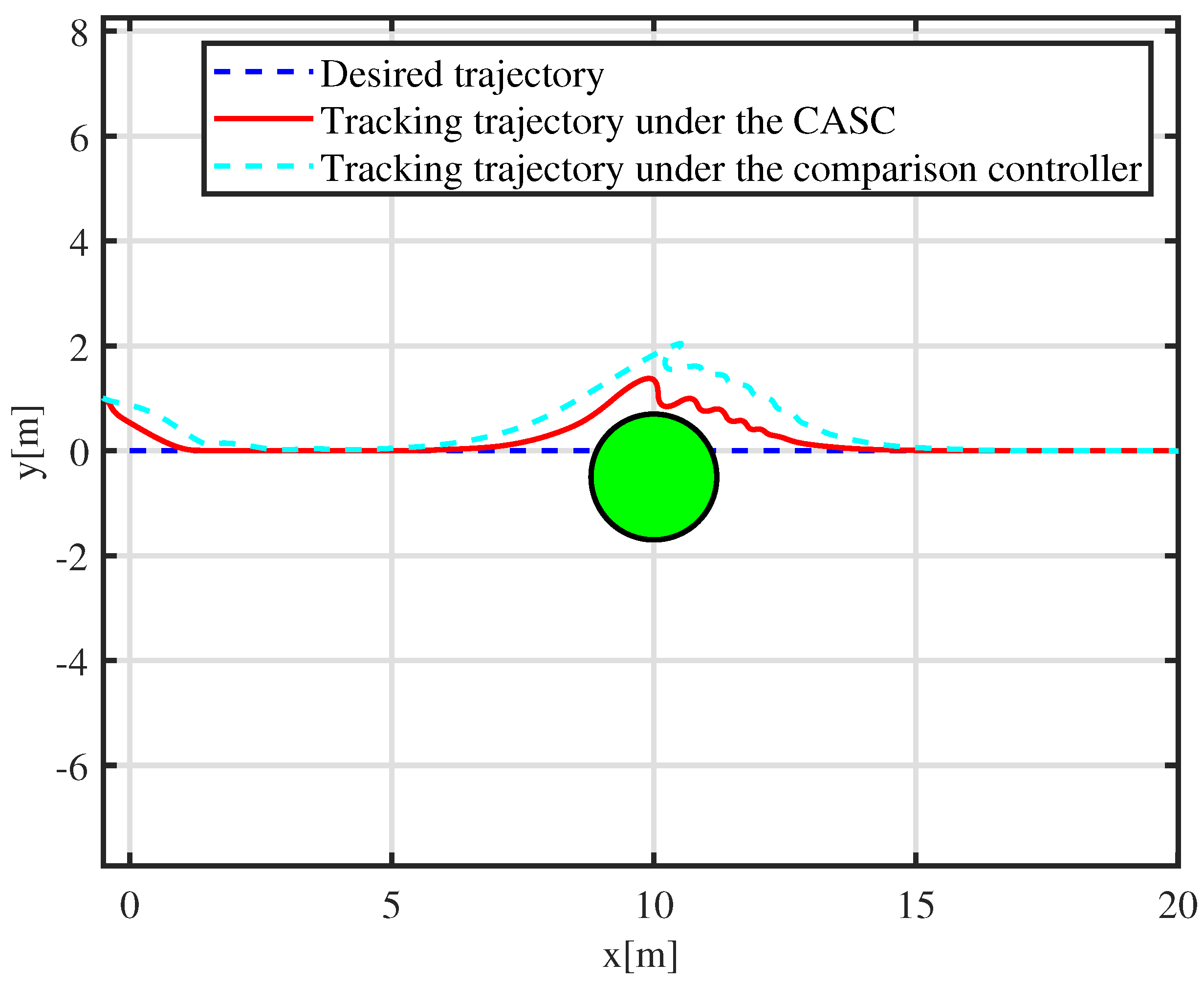
The comparison results are shown in Figure 5 and Figure 6, and simulations are designed using the controller proposed in [31] and the CASC proposed in this paper. The initial posture of the desired trajectory is $[0$ m, 0 m, $0$ rad${]}^T$, and the trajectory is generated via the time-varying velocity vector ${\nu }_d$, and ${\nu }_d={[u_d,v_d,r_d]}^T$: $u_d=0.2$ m/s, $v_d=0$ m/s and $r_d=0$ rad/s for $0\le t<100$ s. The center of the obstacle is (10 m, $-0.5$ m), and the safe collision-avoidance radii is $1.5$ m. As shown in Figure 5, the horizontal axis is the horizontal position, and the vertical coordinate is the vertical position. The dynamically positioned vessel avoids the obstacle and tracks successfully the desired trajectory. This demonstrates that the proposed CASC accomplishes faster convergence and becomes steadily smaller.

Figure 5. Trajectory-tracking-control results under different controllers.

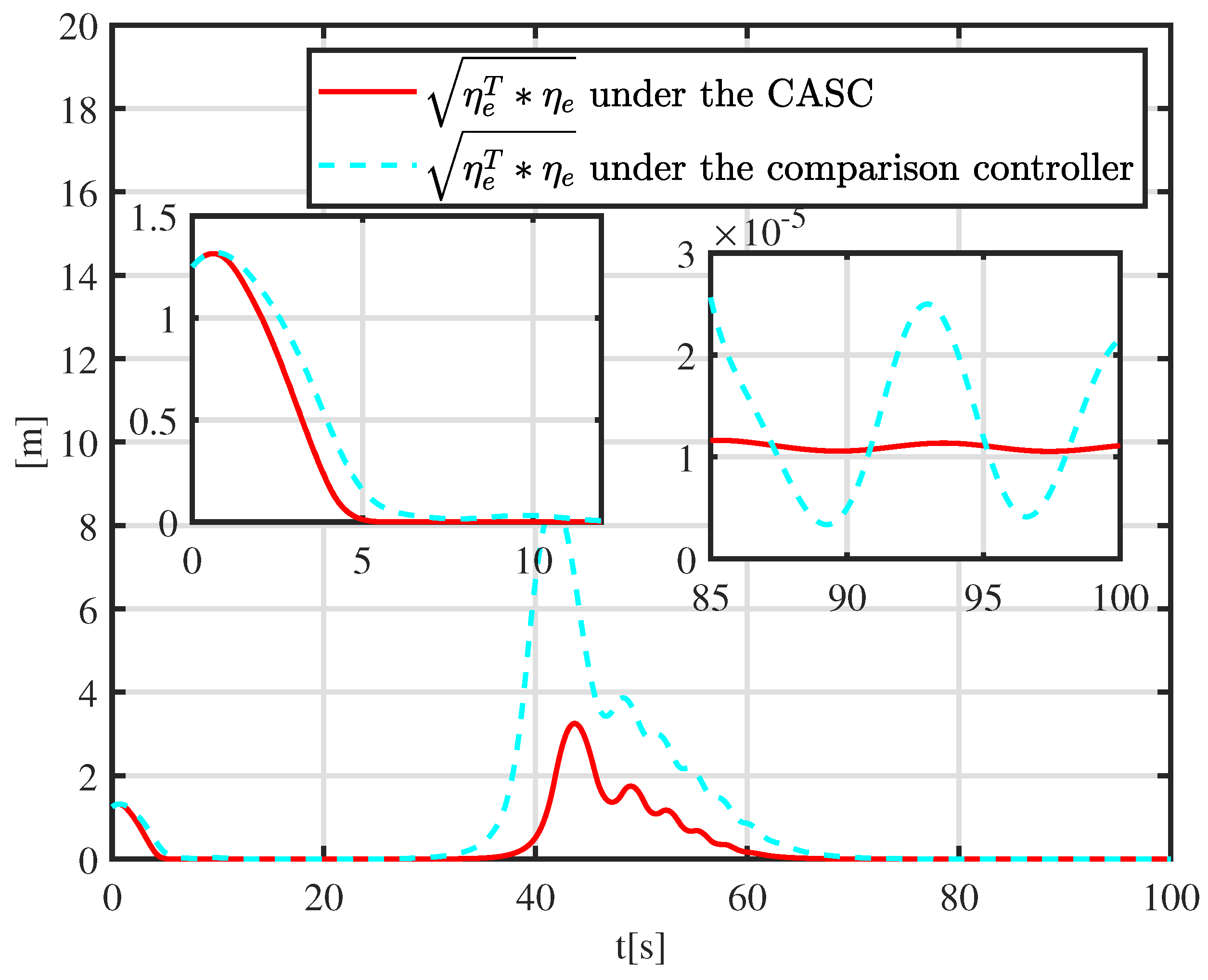
Figure 6. Tracking error function under different controllers.

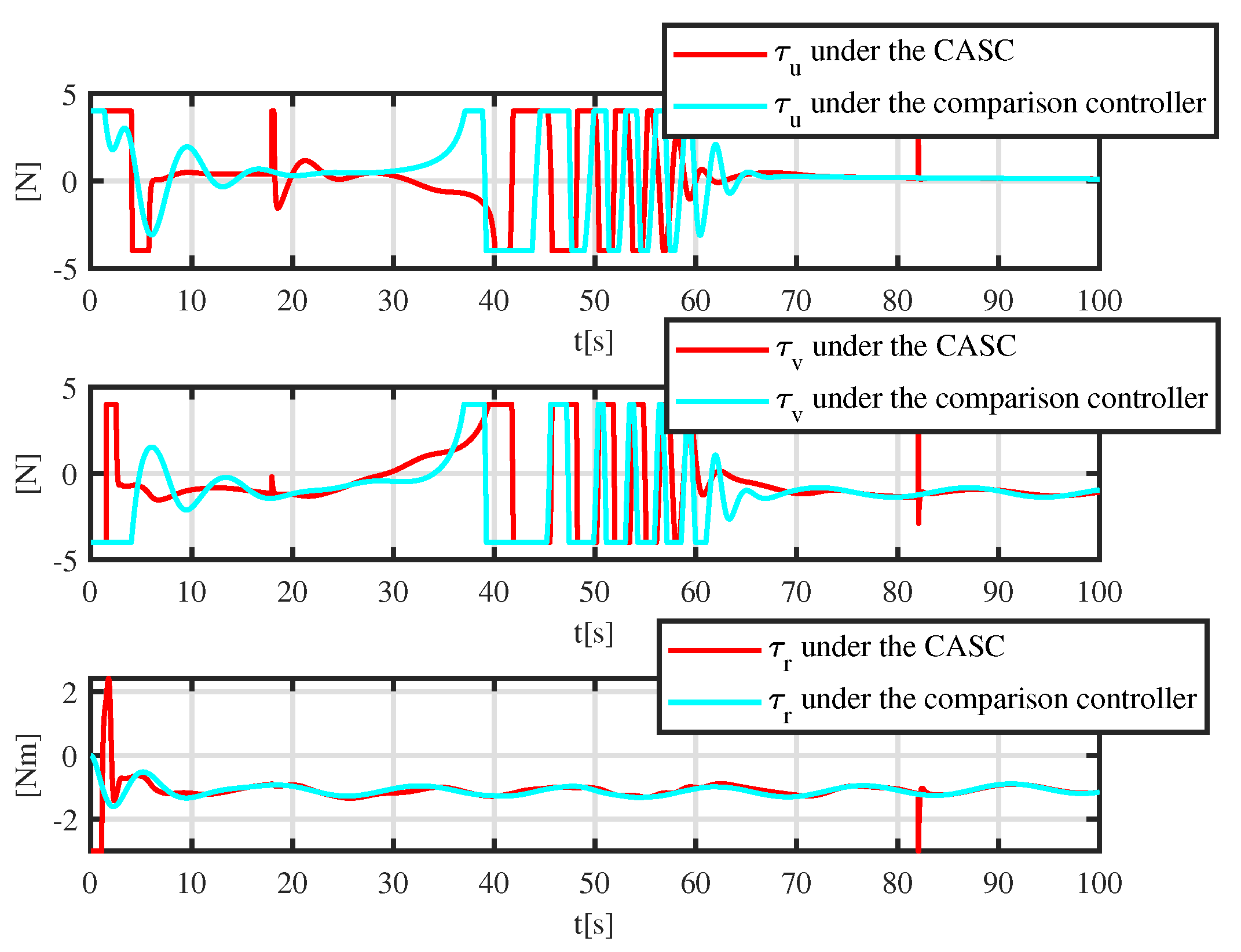
More details are shown in Figure 6. A tracking error function ${\eta }_e=\eta -{\eta }_d$ is employed to show the error-convergence speed under different controllers. At 0–30 s, the tracking error ${\eta }_e$ gradually becomes smaller. During 30–70 s, the dynamically positioned vessel is moving toward the obstacle, and the dynamically positioned vessel avoids the obstacle under different controllers. There are small oscillations in position, which are the result of the co-action of tracking control and the APF. Compared with the controller proposed in [31], the CASC causes smaller oscillations in position, and the tracking error $\sqrt{{\eta }_e^T{\eta }_e}$ converges quickly. At 70–100 s, the dynamically positioned vessel keeps away from the obstacle, the error function $\sqrt{{\eta }_e^T{\eta }_e}$ decreases continuously, and the error goes back to the neighboring zone of zero. Figure 7 shows that the error constraints are achieved when $TC=0$. Figure 8 shows that the control input is limited. At 30–70 s, to avoid obstacle and ensure safe navigation, the CASC gives saturated input signals and makes the ship turn. Figure 9 is the velocity-recovery performance. Note that the initial estimated values of the ESO are set to zero. After a while, the ESO can accurately estimate the velocity of the dynamically positioned vessel. Figure 10 is the estimation performance of the unknown item $\zeta$, and the ESO can accurately estimate item $\zeta$.

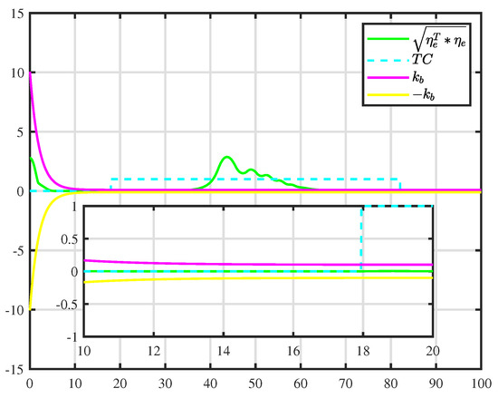
Figure 7. Error constraints for $\sqrt{{\eta }_e^T{\eta }_e}$.

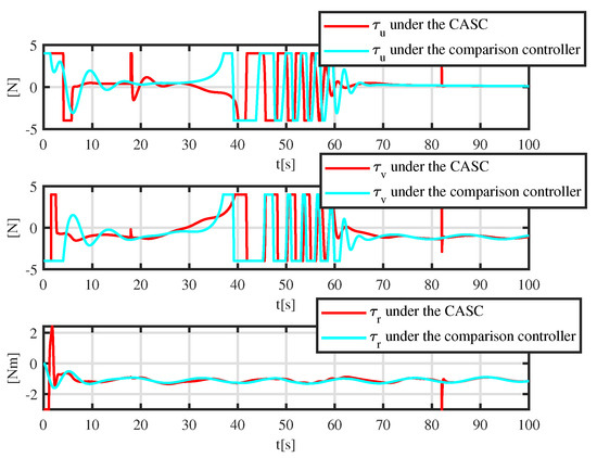
Figure 8. Control input under the controller proposed in [31] and the CASC.

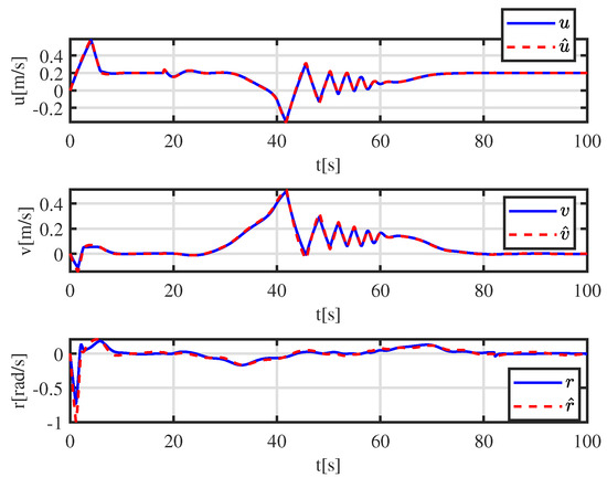
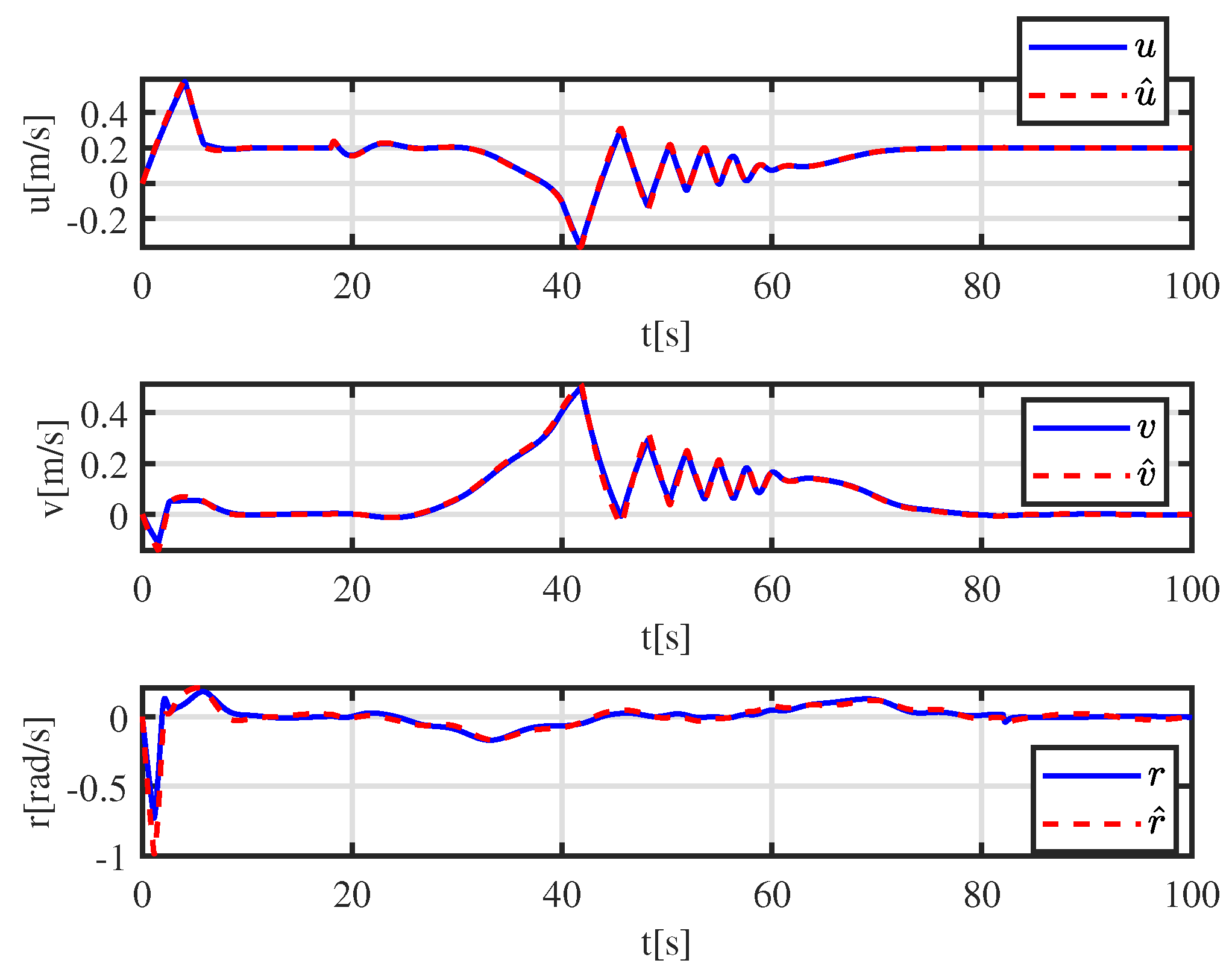
Figure 9. Velocity estimation under the ESO.

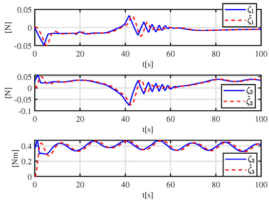
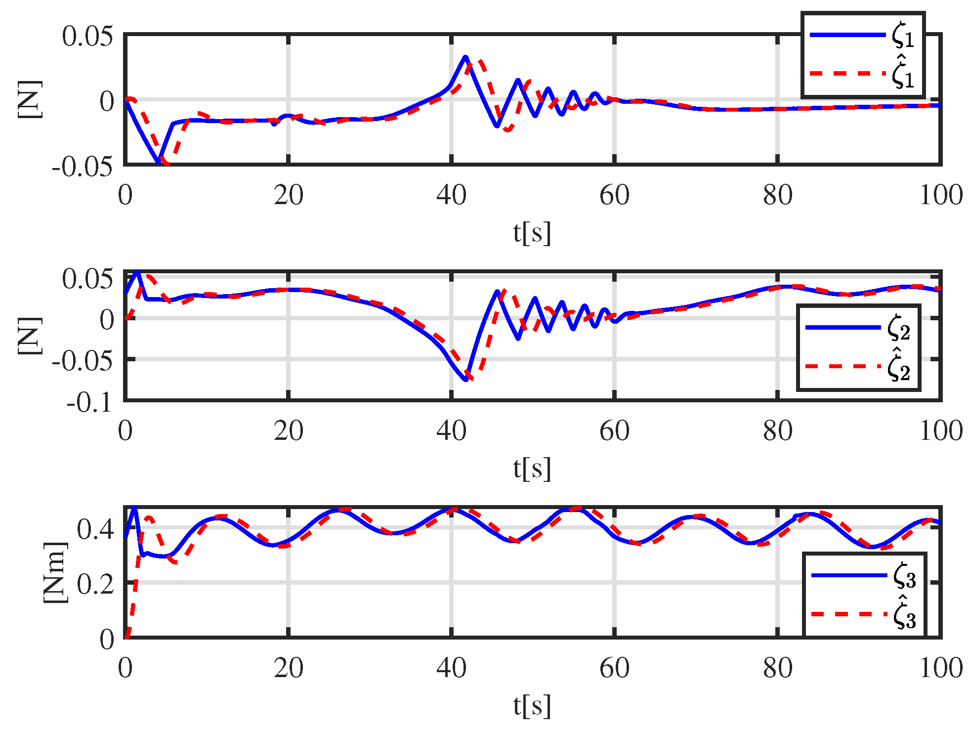
Figure 10. Unknown function and estimation under the ESO.

5.2. Simulation Experiment with a Moving Obstacle

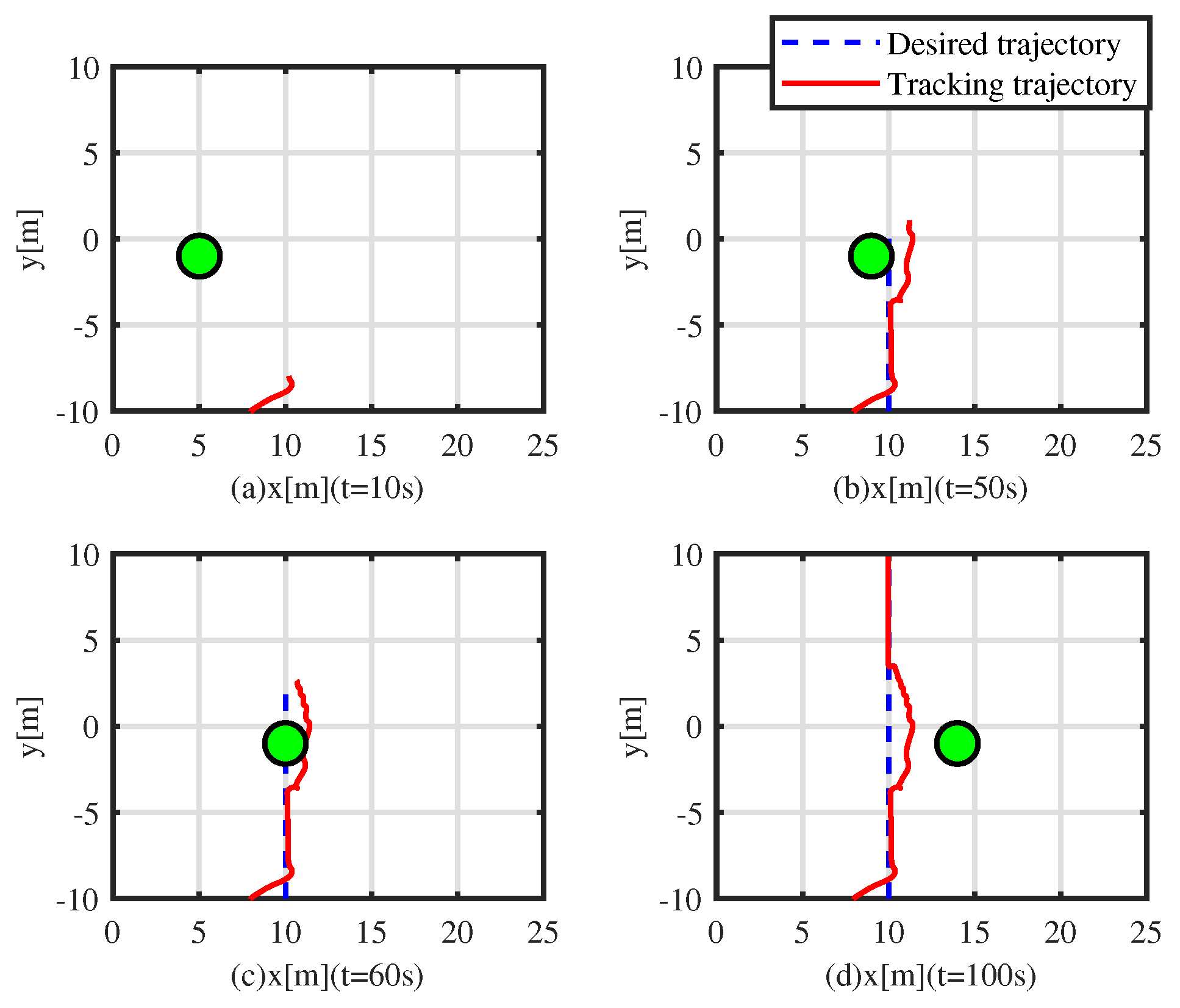
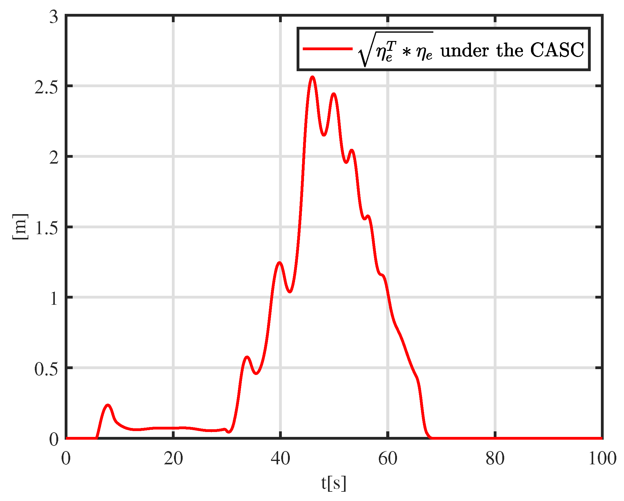
To further appraise the performance of the CASC, a moving obstacle is considered in the simulation experiment. The initial position of the moving obstacle is $[4$ m, $-1$ m, $0$rad${]}^T$, and its velocity is $[0.1$ m/s, 0 m/s, 0 rad/s${]}^T$. Figure 11, Figure 12 and Figure 13 depict the simulation results. Figure 11 shows the tracking results, where the dynamically positioned vessel smoothly avoids obstacles under the CASC. In Figure 11a t = 0–10 s, the dynamically positioned vessel successfully tracks the desired trajectory. The obstacle comes from the port side of the dynamically positioned vessel. In Figure 11b t = 50 s, the dynamically positioned vessel is taking action to avoid collision with the moving obstacle. In Figure 11c, t = 60 s, the dynamically positioned vessel is overtaking the obstacle from its port side. In Figure 11d, t = 100 s, the dynamically positioned vessel is moving away from the moving obstacle. Figure 12 shows the time-varying error $\sqrt{{\eta }_e^T{\eta }_e}$. At t = 0–30 s, the vessel successfully tracks the desired trajectory with a small tracking error. At t = 30–70 s, to avoid obstacles, the tracking error increases gradually and then decreases gradually. At t = 70–100 s, there is no risk of collision, and the tracking error converges to a small compact set. Figure 13 shows that the control inputs are saturated at 0–10 s and 30–70 s. At 0–10 s, due to a large initial tracking error, the control inputs are saturated. At t = 70–100 s, to avoid obstacles, the control inputs suffer from sudden jumps.

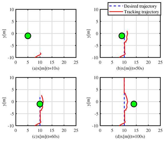
Figure 11. Control results with moving obstacle. (a) Tracking result at $t=10$ s. (b) Tracking result at $t=50$ s. (c) Tracking result at $t=60$ s. (d) Tracking result at $t=100$ s.

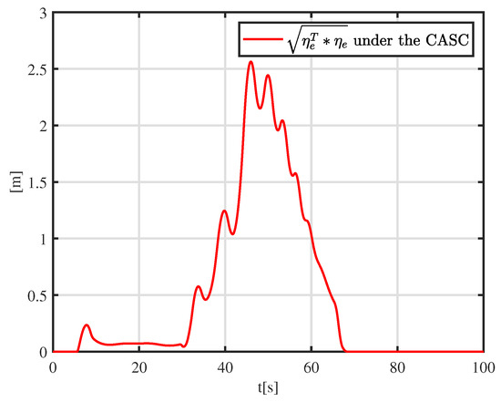
Figure 12. Time-varying error $\sqrt{{\eta }_e^T{\eta }_e}$.

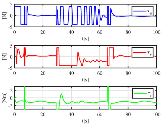
Figure 13. Control input under a moving obstacle.

6. Conclusions

This paper presents a collision-avoidance switch-control strategy for tracking the control of dynamically positioned vessels. To assess the risk of collision avoidance, a calculation of collision risk is introduced into the control design. According to the result of the collision-avoidance risk evaluation, a switch control strategy combined with a collision-avoidance controller and a predefined performance controller is proposed such that all error signals of the system are bounded. Simulation experiments prove that the proposed controller can achieve collision avoidance and predefined performance, even under an environment with dynamic obstacles. When the vessel rotates to avoid collisions, the tracking trajectory is jittery and unsmooth, and the input signals make sudden jumps. Research on collision-avoidance path planning is one of the technologies to handle this problem, which can be treated in future works.

References

- Sørensen, A.J. A survey of dynamic positioning control systems. Annu. Rev. Control 2011, 35, 123–136. [Google Scholar] [CrossRef]
- Cui, J.; Yang, R.; Pang, C.; Zhang, Q. Observer-based adaptive robust stabilization of dynamic positioning ship with delay via Hamiltonian method. Ocean Eng. 2021, 222, 108439. [Google Scholar] [CrossRef]
- Hu, C.; Wu, D.; Liao, Y.; Hu, X. Sliding mode control unified with the uncertainty and disturbance estimator for dynamically positioned vessels subjected to uncertainties and unknown disturbances. Appl. Ocean Res. 2021, 109, 102564. [Google Scholar] [CrossRef]
- Gao, X.; Li, T.; Yuan, L.E.; Bai, W. Robust fuzzy adaptive output feedback optimal tracking control for dynamic positioning of marine vessels with unknown disturbances and uncertain dynamics. Int. J. Fuzzy Syst. 2021, 23, 2283–2296. [Google Scholar] [CrossRef]
- Fossen, T.I. Guidance and Control of Ocean Vehicles; John Wiley & Sons, Inc.: Hoboken, NJ, USA, 1994. [Google Scholar]
- Zhang, Z.Y.; Wu, H.T.; Liu, W.X. Effects of mooring line hydrodynamic coefficients and wave parameters on the floating production storage and offloading motions. Desalin. Water Treat. 2021, 239, 278–288. [Google Scholar] [CrossRef]
- Liu, X.; Miao, Q.; Wang, X.; Xu, S.; Fan, H. A novel numerical method for the hydrodynamic analysis of floating bodies over a sloping bottom. J. Mar. Sci. Technol. 2021, 26, 1198–1216. [Google Scholar] [CrossRef]
- Xia, X.; Yang, Z.; Yang, T. Leader–Follower Formation Tracking Control of Underactuated Surface Vehicles Based on Event-Trigged Control. Appl. Sci. 2023, 13, 7156. [Google Scholar] [CrossRef]
- Shan, Q.; Wang, X.; Li, T.; Chen, C.P. Finite-time control for USV path tracking under input saturation with random disturbances. Appl. Ocean Res. 2023, 138, 103628. [Google Scholar] [CrossRef]
- Van, M.; Do, V.T.; Khyam, M.O.; Do, X.P. Tracking control of uncertain surface vessels with global finite-time convergence. J. Adv. Res. 2021, 241, 109974. [Google Scholar] [CrossRef]
- Zhu, Y.; Zhang, H.; Li, H.; Zhang, J.; Zhang, D. Optimal Jamming Strategy Against Two-state Switched System. IEEE Commun. Lett. 2022, 13, 2283–2296. [Google Scholar] [CrossRef]
- Gao, S.; Xue, J.J. Nonlinear vector model control of underactuated air cushion vehicle based on parameter reduction algorithm. Trans. Inst. Meas. Control 2021, 43, 1202–1211. [Google Scholar] [CrossRef]
- Li, H.; Xu, W.; Zhang, H.; Zhang, J.; Liu, Y. Polynomial regressors based data-driven control for autonomous underwater vehicles. Peer-to-Peer Netw. Appl. 2020, 13, 1767–1775. [Google Scholar] [CrossRef]
- Do, K.D. Global robust and adaptive output feedback dynamic positioning of surface ships. J. Mar. Sci. Appl. 2011, 10, 325–332. [Google Scholar] [CrossRef]
- Fossen, T.I.; Strand, J.P. Passive nonlinear observer design for ships using Lyapunov methods: Full-scale experiments with a supply vessel. Automatica 1999, 35, 3–16. [Google Scholar] [CrossRef]
- Xia, X.; Xia, C.; Sun, C. Distributed formation tracking control of underactuated surface vehicles based on event-trigged control. Trans. Inst. Meas. Control 2023. [Google Scholar] [CrossRef]
- Liu, Y.Y.; Lin, X.G.; Liang, K. Robust tracking control for dynamic positioning ships subject to dynamic safety constraints. Ocean Eng. 2022, 266, 112710. [Google Scholar] [CrossRef]
- Li, J.; Du, J.L.; Hu, X. Robust adaptive prescribed performance control for dynamic positioning of ships under unknown disturbances and input constraints. Ocean Eng. 2020, 206, 107254. [Google Scholar] [CrossRef]
- Zhu, G.; Du, J. Global Robust Adaptive Trajectory Tracking Control for Surface Ships Under Input Saturation. IEEE J. Ocean. Eng. 2020, 45, 442–450. [Google Scholar] [CrossRef]
- Qin, H.; Li, C.; Sun, Y.; Li, X.; Du, Y.; Deng, Z. Finite-time trajectory tracking control of unmanned surface vessel with error constraints and input saturations. J. Frankl. Inst. 2020, 357, 11472–11495. [Google Scholar] [CrossRef]
- Du, J.L.; Hu, X.; Krstic, M.; Sun, Y.Q. Robust dynamic positioning of ships with disturbances under input saturation. Automatica 2016, 73, 207–214. [Google Scholar] [CrossRef]
- Qin, H.D.; Li, C.P.; Sun, Y.C.; Wang, N. Adaptive trajectory tracking algorithm of unmanned dinamicaly positioned vessel based on 269 anti-windup compensator with full-state constraints. Ocean Eng. 2020, 200, 106906. [Google Scholar] [CrossRef]
- Su, Y.; Gong, C.; Zhang, D.; Hu, X. Simple Dynamic Positioning Control Design for Surface Vessels with Input Saturation and External Disturbances. IEEE Trans. Circuits Syst. II Express Briefs 2023, 70, 1530–1534. [Google Scholar] [CrossRef]
- Bechlioulis, C.P.; Rovithakis, G.A. Robust adaptive control of feedback linearizable MIMO nonlinear systems with prescribed performance. IEEE Trans. Autom. Control 2008, 53, 2090–2099. [Google Scholar] [CrossRef]
- Wang, X.J.; Yin, X.H.; Shen, F. Disturbance observer based adaptive neural prescribed performance control for a class of uncertain nonlinear systems with unknown backlash-like hysteresis. Neurocomputing 2018, 299, 10–19. [Google Scholar] [CrossRef]
- Xia, G.Q.; Zhang, B.W. Finite-Time Control of dinamicaly positioned vessel Based on Disturbance Observer. Math. Probl. Eng. 2022, 2022, 9262457. [Google Scholar] [CrossRef]
- Tam, C.K.; Bucknall, R. Cooperative path planning algorithm for marine dinamicaly positioned vessels. Ocean Eng. 2013, 57, 25–33. [Google Scholar] [CrossRef]
- Peng, Z.; Wang, D.; Li, T.; Han, M. Output-Feedback Cooperative Formation Maneuvering of Autonomous dynamic positioning 273 Vehicles With Connectivity Preservation and Collision Avoidance. IEEE Trans. Cybern. 2020, 50, 2527–2535. [Google Scholar] [CrossRef]
- Park, B.S.; Yoo, S.J. An error transformation approach for connectivity-preserving and collision-avoiding formation tracking of networked uncertain underactuated surface vessels. IEEE Trans. Cybern. 2019, 49, 353–359. [Google Scholar] [CrossRef]
- Park, B.S.; Yoo, S.J. Distributed dynamic obstacle avoidance design to connectivity-preserving formation control of uncertain underactuated surface vehicles under a directed network. Ocean Eng. 2023, 273, 113872. [Google Scholar]
- Zhang, B.W.; Xia, G.Q. Output Feedback Tracking Control with Collision Avoidance for Dynamic Positioning Vessel under Input Constraint. J. Mar. Sci. Eng. 2023, 11, 811. [Google Scholar] [CrossRef]
- Zhang, K.; Huang, L.; He, Y.; Wang, B.; Chen, J.; Tian, Y.; Zhao, X. A real-time multi-ship collision avoidance decision-making system for autonomous ships considering ship motion uncertainty. J. Mar. Sci. Eng. 2023, 278, 114205. [Google Scholar] [CrossRef]
- Ahmed, Y.A.; Hannan, M.A.; Oraby, M.Y.; Maimun, A. COLREGs compliant Fuzzy-Based collision avoidance system for multiple ship encounters. J. Mar. Sci. Eng. 2021, 9, 790. [Google Scholar] [CrossRef]
- Chiang, H.T.L.; Tapia, L. COLREG-RRT: An RRT-based COLREGS-compliant motion planner for surface vehicle navigation. IEEE Robot. Autom. Lett. 2018, 3, 2024–2031. [Google Scholar] [CrossRef]
- He, Y.; Jin, Y.; Huang, L.; Xiong, Y.; Chen, P.; Mou, J. Quantitative analysis of COLREG rules and seamanship for autonomous collision avoidance at open sea. Ocean Eng. 2017, 140, 281–291. [Google Scholar] [CrossRef]
- Skjetne, R.; Fossen, T.I.; Kokotovi, P.V. Adaptive maneuvering, with experiments, for a model ship in a marine control laboratory. Automatica 2005, 41, 289–298. [Google Scholar] [CrossRef]
Disclaimer/Publisher’s Note: The statements, opinions and data contained in all publications are solely those of the individual author(s) and contributor(s) and not of MDPI and/or the editor(s). MDPI and/or the editor(s) disclaim responsibility for any injury to people or property resulting from any ideas, methods, instructions or products referred to in the content. |
© 2023 by the authors. Licensee MDPI, Basel, Switzerland. This article is an open access article distributed under the terms and conditions of the Creative Commons Attribution (CC BY) license (https://creativecommons.org/licenses/by/4.0/).