Abstract
When examining the history of wind engineering, it is evident that many full-scale/model test comparisons have found noticeable differences between the results. Although understanding the causes of these differences is important for practical purposes, limited numerical and experimental conditions have often resulted in subjective explanations for full-scale/model test comparisons without scientific validation. To address this issue, this article suggests the use of the computational fluid dynamics technique or the multiple-fan actively controlled wind tunnel technique to quantitatively reveal the adverse effects that impact the reliability of the traditional atmospheric boundary layer wind tunnel tests for a large cooling tower, including not only the widely acknowledged influences (Reynolds number effects and turbulent flow characteristics effects) but also the non-stationarity effects that have potential influences. Established on the novel proposition, a new research scheme for future full-scale/model test wind effects comparisons for large cooling towers has been formulated based on the numerical or physical simulations of the sinusoidal flow fields. Using the Pengcheng cooling tower as a case study, the research recognized the very significant impact of Reynolds number effects, the non-stationarity effects that cannot be ignored, and the negligible effects of turbulent flow characteristics.
1. Introduction
Over the past 50 years, the wind engineering community has relied heavily on the traditional atmospheric boundary layer (ABL) wind tunnel simulation technique for scientific research and engineering practices. This technique has yielded theoretical achievements and ensured the safety of numerous engineering structures against strong winds. However, the reliability of ABL wind tunnel model tests has become a major concern of the wind engineering community. Countless studies have attempted to validate this simulation technique by comparing the model test and the full-scale measurement data of various engineering structures, with the results disseminated through the literature. Through extensive literature review, it becomes apparent that most full-scale/model test comparisons lead to noticeable discrepancies between the full-scale measurement results and wind tunnel data. These discrepancies can take various forms, including underestimation of mean and/or peak negative pressures at flow separation regions on low-rise building models’ roofs [1,2,3,4,5,6], differing local fluctuating pressures due to vortex shedding on high-rise building models [7], underestimation of dynamic structural responses in the intermediate-frequency range for aero-elastic model tests on high-rise buildings [8], differences in the root-mean-square acceleration between full-scale measurements and force balance model tests for high-rise buildings [9,10,11,12,13], much lower vertical-vortex-induced vibration amplitudes for long-span bridges obtained through section models and aero-elastic models compared to those observed on prototypes [14,15], non-Gaussian pressure fluctuations on prototypes compared to Gaussian-distributed model test samples [13,16,17], and stronger coherences between wind pressure samples at different locations during model tests than full-scale measurements [17,18]. Details of the above-mentioned full-scale/model test comparisons are listed in Table 1 for reference.

Table 1.
Representative full-scale/model test comparisons with noticeable differences in results.
Numerous researchers have attempted to explain the observed full-scale/model test discrepancies. Richards et al. [19] attributed these discrepancies to the turbulence, the velocity profile, and Reynolds number (Re). Li et al. [15] linked the full-scale/model test discrepancy of the suspension bridge to Re effects and flow pattern differences. Chen et al. [20] proposed that the difference in a stadium’s dynamic response between the prototype measurements and the prediction using model test data and finite element calculations may result from inaccuracies in full-scale measurements, inaccurately modeled wind loads on the stadium roof in the wind tunnel, wind direction differences, turbulence intensity and scale mismatches between the two experiments, damping issues, and limitations in finite element simulation. Dalgliesh [21] suggested that the observed discrepancies in comparing field measurement results on the 34-story office building in downtown Montreal with wind tunnel data resulted from the difficulty in establishing a static reference pressure for full-scale measurements, the inadequate simulation of the realistic wind velocity in the wind tunnel, and the lack of stationarity and homogeneity of the full-scale velocity field. Huang et al. [1] proposed that their full-scale/model test discrepancies observed were likely due to inadequate simulation of turbulence intensities in the wind tunnel, small-scale turbulence content in the wind tunnel, inaccurate details of the scaled model, different stationary features of the oncoming flow between the two experiments, Re effects, and Jensen number effects.
It is evident that the wind engineering community has consistently identified three main similarity problems that adversely affect the reliability of the traditional ABL wind tunnel simulation technique. Firstly, the use of passive simulation devices (spires and roughness elements) means that the complete turbulent flow characteristics of the realistic ABL flow field cannot be accurately simulated in the wind tunnel (referred to as turbulent flow characteristics effects). Secondly, Re effects exist for wind tunnel tests. Thirdly, the non-stationary features of the realistic ABL winds cannot be accurately simulated in a traditional passive wind tunnel (referred to as non-stationarity effects). A definition of authority for a non-stationary sample refers to a sequence that contains the trend, the seasonality, and/or the periodicity in terms of mathematics [22], which is extremely common in the field of wind engineering. As reported above, Richards et al. [19], Li et al. [15], and Chen et al. [20] suggested that both Re effects and turbulent flow characteristics effects existed, whereas Dalgliesh [21] attributed the observed differences to non-stationarity effects. Huang et al. [1] believed that all three adverse effects were present.
It is important to note that researchers’ explanations for the causes of the observed full-scale/model test differences are all based on subjective conjectures without reliable scientific validation, and some of their explanations are in disagreement with one another. Future efforts should be made to validate these conjectures using reliable data. In practice, Re effects, turbulent flow characteristics effects, and non-stationarity effects should be respectively quantified under a unified scientific scheme for structures, such as large cooling towers. Only then can the most significant similarity problem with the traditional ABL wind tunnel simulation technique be identified and addressed. Moreover, it is essential to acknowledge the limitations of previous studies in revealing the most significant similarity problem due to the difficulty of separating the mingled adverse effects under conventional numerical and experimental conditions. In response, this article proposes a new research scheme for future full-scale/model test comparisons that utilizes the computational fluid dynamics (CFD) technique or the multiple-fan actively controlled wind tunnel technique based on sinusoidal flow field simulations and validates the proposal using a specific case study of Pengcheng cooling tower.
2. A New Research Scheme for Full-Scale/Model Test Comparisons Based on Numerical and Physical Sinusoidal Flow Field Simulations
2.1. New Research Scheme Proposal
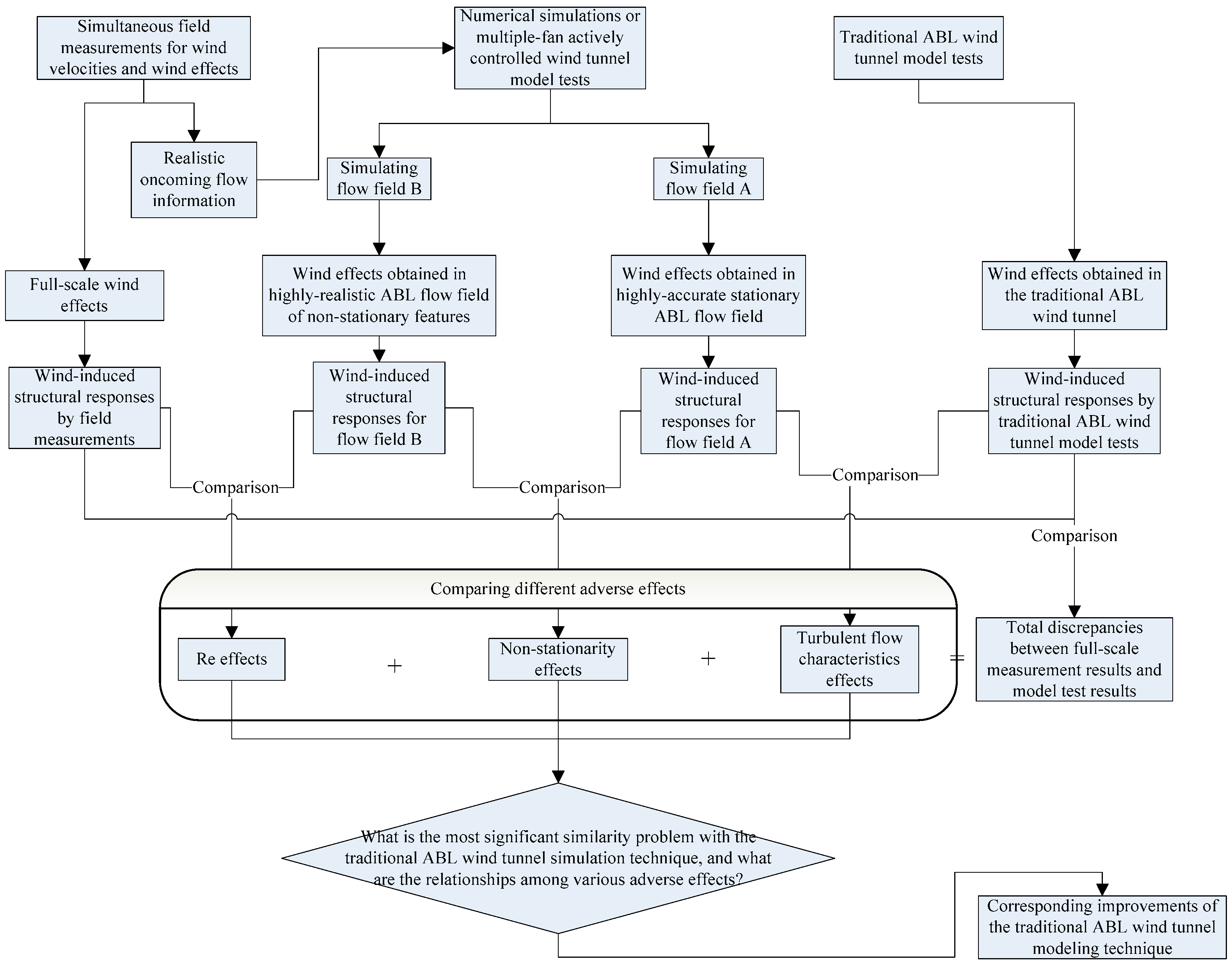
By following the below-mentioned procedures, the proposed new research scheme can effectively discern the intertwined adverse effects for full-scale/model test comparisons for structures such as large cooling towers:
Step 1: Simultaneously measuring the meteorological wind data and wind effects on structures on the prototype and conducting corresponding model tests on the scaled models without the Re effects simulation in the traditional ABL wind tunnel;
Step 2: Creating a highly accurate (with the ABL turbulence characteristics accurately simulated according to the field measurement results) stationary ABL flow field at a low Re (flow field A) and a highly realistic non-stationary ABL flow field at a low Re (flow field B) on a CFD platform or in a multiple-fan actively controlled wind tunnel using measured meteorological wind data, and performing model tests in both flow fields;
Step 3: Compute the structural responses to wind loads in various flow fields, including flow fields A and B, the flow field simulated in the traditional ABL wind tunnel, and the realistic flow field;
Step 4: Compare wind-induced structural responses based on in situ measurements with those based on traditional wind tunnel model tests. This will help quantify the total discrepancies, including Re effects, turbulent flow characteristics effects, and non-stationarity effects. Then, analyze the structural responses based on model tests conducted in flow fields A and B to separate these adverse effects. Specifically, quantify Re effects by comparing structural responses for full-scale measurements to those for model tests conducted in flow field B. Non-stationarity effects should be quantified by comparing structural responses for the model test conducted in flow field A to those for the model test conducted in flow field B. Turbulent flow characteristics effects should be quantified by comparing structural responses for the model test conducted in flow field A to those for the traditional wind tunnel model test;
Step 5: Determine the most significant adverse influence on the reliability of the traditional ABL wind tunnel simulation technique by comparing the three adverse effects.
Figure 1 showcases the flowchart of the new research scheme, which heavily relies on the abilities of the CFD technique and the multiple-fan actively controlled wind tunnel technique in simulating the non-stationary flow fields.

Figure 1.
Flowchart of the new research scheme.
2.2. Capabilities of CFD Technique and Multiple-Fan Actively Controlled Wind Tunnel Technique Reported in the Literature
According to ref. [23], a flow field is simulated by inputting the inlet velocity varied in accordance with a non-stationary wind speed time-history measured near Shenzhen Baoan Stadium on the commercial CFD platform Fluent utilizing the user-defined function (UDF) module provided by the numerical platform. The pressure field on a low-rise building in that flow field is then calculated and compared with that calculated in a stationary flow field. When the numerical simulation is completed, the velocity samples calculated are not directly compared with the simulation target by ref. [23] to validate the simulation accuracy before use.
With respect to the physical tests, the concept of actively controlled wind tunnels was first proposed in the 1970s, and some researchers have since realized flow control in wind tunnels to mitigate some issues with the traditional ABL wind tunnel simulation technique, such as low turbulence intensity and small-scale turbulence content. However, most of these researchers relied on actively controlled devices placed at the beginning of the traditional wind tunnel to adjust the simulated flow, which technically falls under semi-actively controlled methods. To date, only researchers from Miyazaki University have realized actively controlled wind tunnel model tests in the true sense [24,25]. With the concept of flow production control, two 3-D and one 2-D multiple-fan actively controlled wind tunnels were constructed at Miyazaki University. According to Cao et al. [24], a 3-D multiple-fan actively controlled wind tunnel at Miyazaki University is an open-circuit wind tunnel with 99 fans, each with a diameter of 270 mm, arranged in a 9 × 11 matrix. The test section is 15.5 m long, 2.6 m wide, and 1.8 m high, and the fans are driven by high-quality alternating current servo-motors through a computer, allowing them to be controlled at different frequencies of up to approximately 25 Hz. This enables fluctuating air flow in the test section, and, since the 99 fans can be programmed independently to deliver variable flows, phase shifts can be introduced among the fans, allowing transverse and vertical turbulence to be generated. Using the power spectrum modification method or time-lag modification method [25], highly accurate stationary ABL flow fields were simulated in multiple-fan wind tunnels, with turbulence parameter profiles and Re stress identical to the targets [25]. Furthermore, by repeated modification of both power spectrum and phase of the input data to the fans, Cao et al. [24] achieved simulation of velocity histories with sharp velocity changes. The power spectrum modification method adopted by Refs. [24,25] in simulating non-stationary velocity fields follows the procedures below:
- (1)
- Transform the velocity history into voltage data proportionally, and input the data to the motors of the fans through AD converters. Because of the mechanical inertia of the rotating parts of the motor and because of the inertia of the air inside the tunnel, the velocity history generated cannot be the same as the voltage data history inputted to the motors;
- (2)
- Modify the input data of the fans and drive the fans with new input data. Mathematically, the velocity history can be expanded to be the sum of a series in the frequency domain by fast Fourier transform (FFT). If the power spectrum and phase of the generated velocity history agree with the target ones well at each frequency, the generated velocity history will be very similar to the target one, and high correlation will be achieved between them. Thus, modification of the input data includes the modifications of power spectrum and phase. The methods are expressed in Equations (1) and (2):where is the frequency, , are the power spectrum and phase of the generated flow resulted from the input data with and , and and are the target power spectrum and phase. By conducting inverse FFT with and , new input data of the fans can be obtained;
- (3)
- Repeat the modification of the input data of the fans until satisfactory results are achieved. Modification of the input data should be repeated several times until satisfactory results can be achieved.
2.3. Capabilities of CFD Technique and Multiple-Fan Actively Controlled Wind Tunnel Technique According to the Present Research
On the Fluent 6.2.16 platform, we tried to reproduce the non-stationary flow field for Pengcheng cooling tower site based on a velocity sample measured on location [26] employing the simulation approach reported in ref. [23]. After the numerical simulation, it is found that the simulated velocity samples near the inlet are close to the input velocity time-history (the simulation target); however, when the simulated sample is extracted from a location far away from the inlet, it deviates from the simulation target in both frequency and time domains. The possible reason behind this observation is that numerical simulations are based on mathematical assumptions and approximations of the complicated realistic flow physics, and therefore contain the inherent inaccuracies. Moreover, the computational cost is high for such a simulation approach, and the solution always comes out from the program after a long time of calculation. On the other hand, we also simulated several sinusoidal wave flow fields and found that most simulated results across the computational domain agree well with the simulation target, suggesting the good ability of the numerical platform in simulating rather simple flow events.
In recent years, a multiple-fan actively controlled wind tunnel called TJ-6 has been constructed at Tongji University in Shanghai, China, as shown in Figure 2. TJ-6 has 120 independently controlled highly sensitive fans arranged in a 10 × 12 matrix, with a test section size of 1.8 × 1.5 m and an applied wind speed range of 2.0–20 m/s. However, preliminary investigations have also revealed that TJ-6 cannot easily simulate realistic target velocity histories with sharp velocity changes (typical non-stationary velocity histories), as achieved by Cao et al. [24]. After technical condition evaluations, it was found that the fans in TJ-6 wind tunnel neither do have sufficient stiffness to accurately deliver the targeted complicated non-stationary flows. However, it was also noted that TJ-6 can accurately simulate longitudinal velocity histories that vary according to basic sinusoidal functions, as reported in ref. [27]. According to ref. [27], basic sinusoidal functions are those that can be mathematically expressed as , while senior sinusoidal functions are those obtained via the linear superposition of several basic sinusoidal functions, e.g., the function .
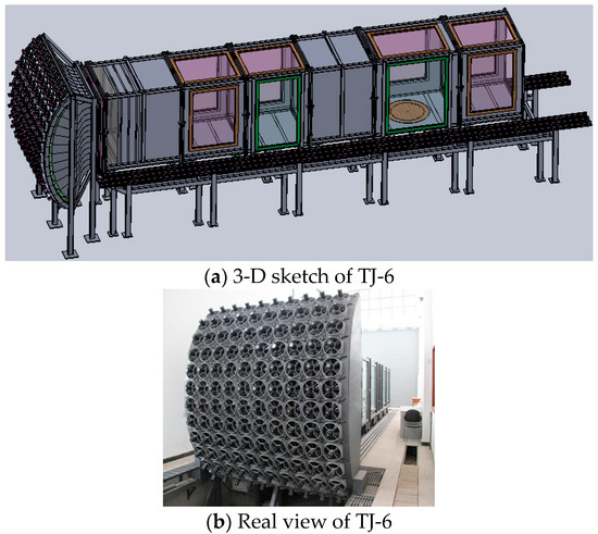
Figure 2.
TJ-6 actively controlled wind tunnel.
In sum, the research scheme proposed in Section 2.1 cannot be undertaken as planned on a commercial CFD platform or in a TJ-6 wind tunnel due to the incapability of both numerical and physical approaches. However, shall we use the abilities of the commercial CFD platform and TJ-6 wind tunnel in accurately simulating the simple sinusoidal wave flow fields to subtly address the aforementioned technical issue of simulating the complicated non-stationary flow fields? This question is answered via in-depth numerical simulations below based on the specific case study of Pengcheng cooling tower.
3. Comparison Based on Numerical Simulation
3.1. Engineering Background and Field Measurements
The Pengcheng cooling tower, located in Pengcheng electric power station in Xuzhou, China, stands at a height of 167 m with a smooth-walled exterior. The tower has a neighboring tower of the same size located to the south with a center-to-center distance of 1.5 times the diameter of the tower base. Additionally, there is a large building complex located to the west. When the wind affects the tower from east or north, there are no major interfering buildings or topography; thus, the flow event can be considered a free-standing tower case.
In 2009, 36 pressure measurement transducers were evenly distributed around the tower’s throat section at a height of 130 m. From 2009 to 2015, wind pressures were measured on the tower two to three times per year for a two-week period each time. Over 4000 h of effective wind pressure samples were collected on the tower under standard ABL strong winds. Samples for the free-standing tower case recorded on 29 November 2011 were chosen from this database for further use. The reason for selecting data collected at that time is explained in ref. [17], which will not be reiterated in this article. Moreover, a typical non-stationary wind velocity sample is extracted from a full-scale wind pressure sample measured in the quasi-steady region on the actual large cooling tower using the approach presented in ref. [26] for further use.
3.2. Numerical Simulation of Non-Stationary Flow Field
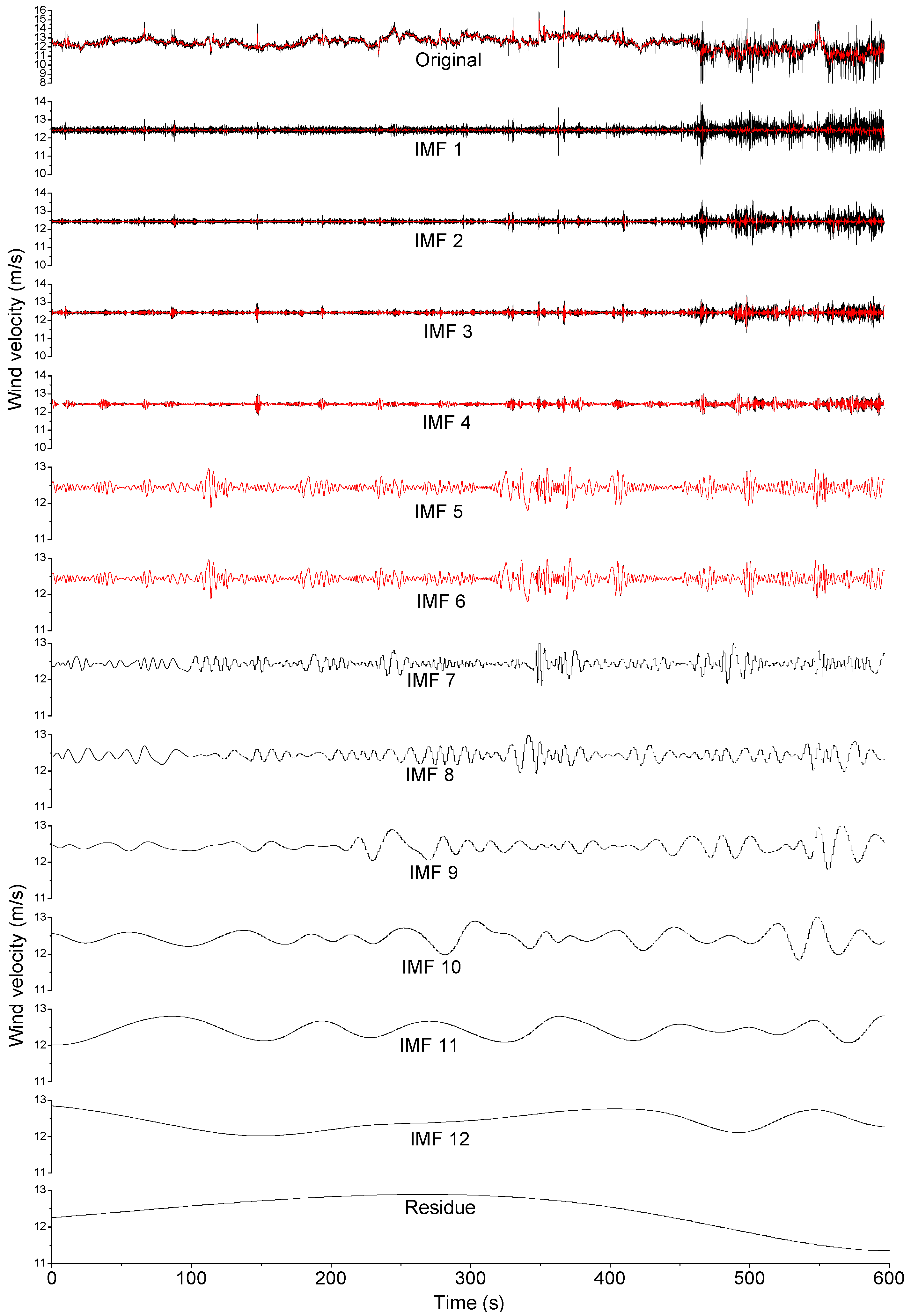
To simulate flow field B, we linearly decomposed an original non-stationary wind velocity sample measured at the Pengcheng power station engineering site on 29 November 2011 into intrinsic mode functions (IMFs) with varying dominant frequencies using the empirical mode decomposition technique first [17], as depicted in Figure 3. To illustrate the energy distributions of different components obtained, FFTs are applied to these IMFs, and the results in the form of amplitude spectral densities (ASDs) are shown in Figure 4. For the spectra obtained to be less noisy and discernable, the original time-history and IMFs 1–6 (the black curves shown in Figure 3) are smoothed using the five-point FFT technique to generate the new samples for use (the red curves shown in Figure 3) before being transformed into ASDs. As can be seen in Figure 4a, among these high-frequency IMFs (IMFs 1–5), only IMF 1 possesses the commensurate energy in the high-frequency domain (5–10 Hz) compared with the original velocity sample. However, all the low-frequency IMFs (IMFs 7–12) and the residue have the same ASDs in the low-frequency domain (0.001–0.01 Hz) compared with the original velocity sample (see Figure 4b). According to ref. [17], all these low-frequency IMFs and the residue should be responsible for the non-stationarity of the original velocity sample. To reconstruct the original velocity sample, IMFs 1 and 7–12 and the residue should be employed based on the linear superposition method with respect to the energy distribution of the reconstructed sample in the full frequency domain and the non-stationary feature of the reconstructed sample.
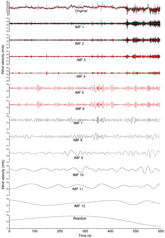
Figure 3.
EMD decomposition of the wind velocity sample measured in the field.
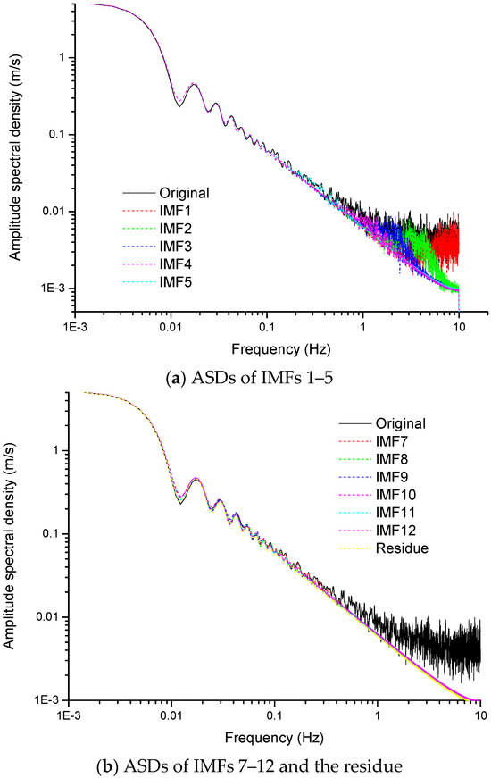
Figure 4.
ASDs of the original velocity sample and different components obtained from EMD decomposition.
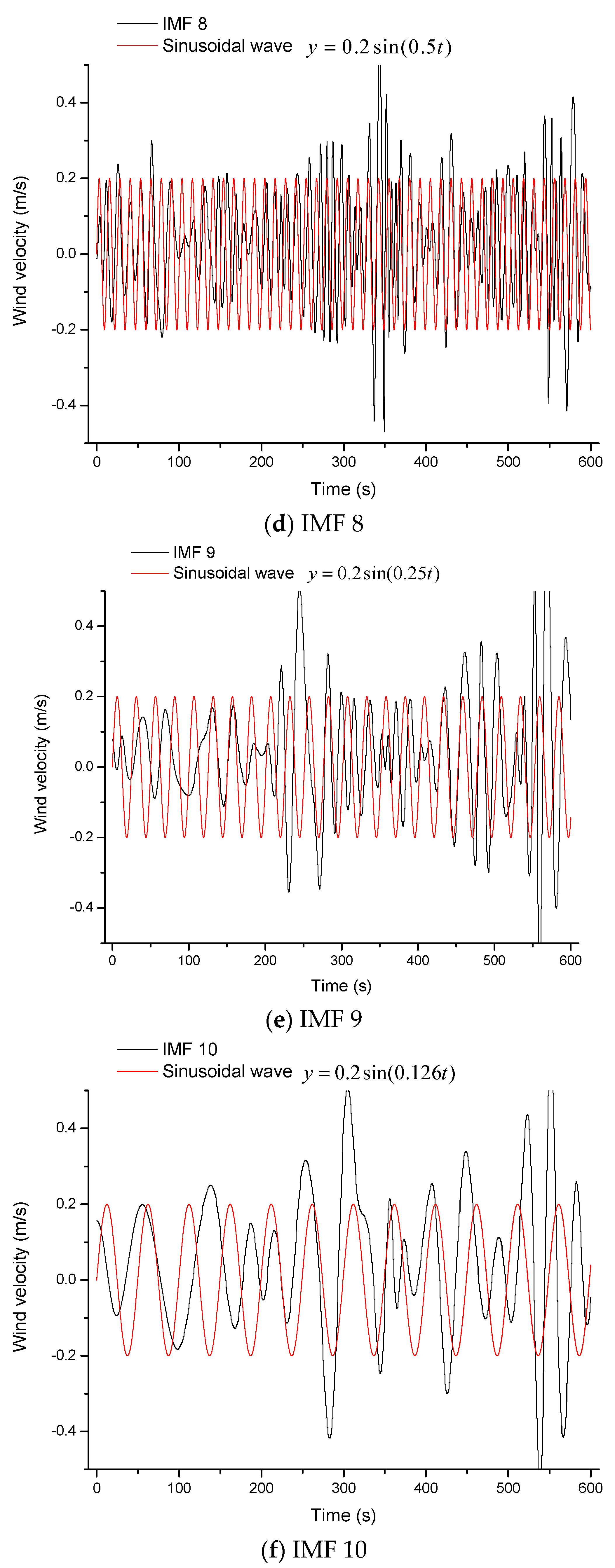
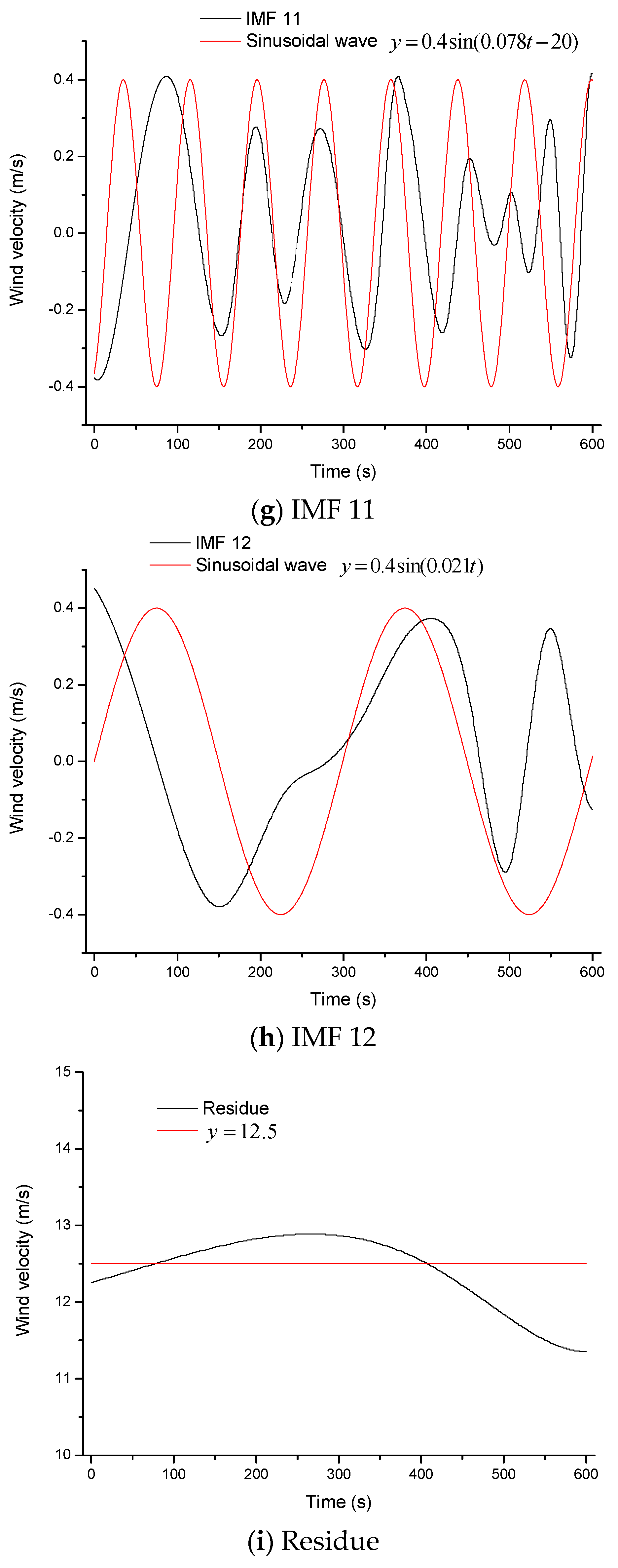
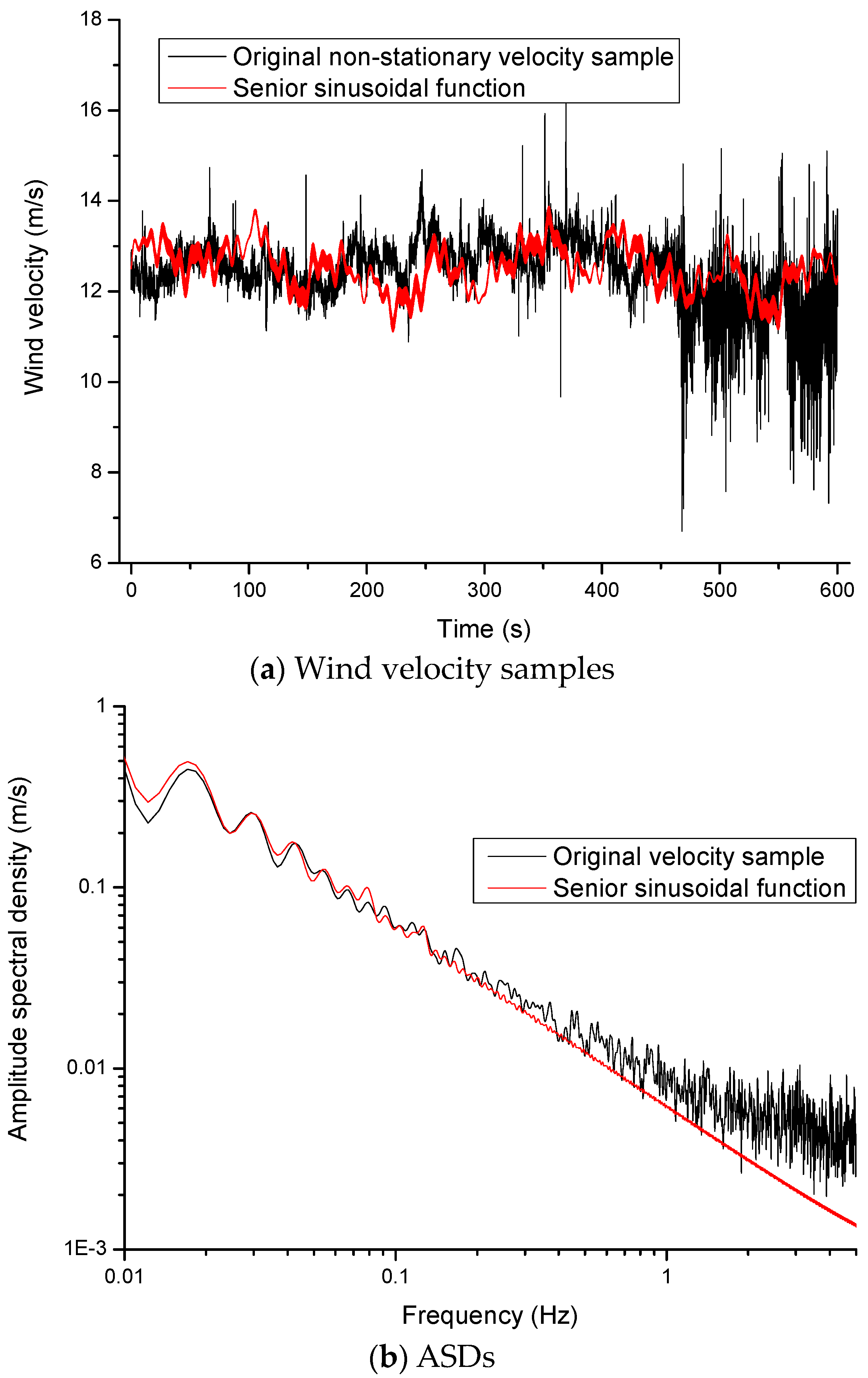
To transform the non-stationary velocity sample into a sinusoidal function, the resulting IMFs (IMFs 1, 7–12, and the residue) were then approximated using basic sinusoidal waves with different periods (see Figure 5). To illustrate this point further, we can look at the basic sinusoidal wave for IMF 11 shown in Figure 5g. The comparison of the two curves in Figure 5g demonstrates that the basic sinusoidal wave for IMF 11, which is represented by the equation (where y is the wind velocity in m/s and t is time in seconds), closely resembles IMF 11 in the time domain in terms of the period and the amplitude. Additionally, it is found that the amplitude spectral density of IMF 11 overlaps that of the basic sinusoidal wave in the frequency domain, indicating that IMF 11 and its basic sinusoidal wave possess comparable energy. The same observation can be made for the basic sinusoidal waves associated with other IMFs (see Figure 5). Table 2 lists the amplitude, the frequency, and the phase of all components. Based on the above analyses, we finally obtain a senior sinusoidal function obtained by the linear superposition of all basic sinusoidal functions shown in Figure 5, written as Equation (3). This senior sinusoidal function can well approximate the original non-stationary velocity sample measured at the Pengcheng power station engineering site. As shown in Figure 6, the original non-stationary velocity sample and the simulated senior sinusoidal function are basically close together in both the time and frequency domains, suggesting the validity of the proposed method in simulating the non-stationary flow field. Although the evidence approximately holds for the linear superposition practice to simulate the non-stationary flow field, only one specific case is considered, and more rigorous examinations will be performed in the future in order to make the general claims about the proposed simulation method. At present, we restrict the claim to the flow around Pengcheng cooling tower in the specific wind environment.
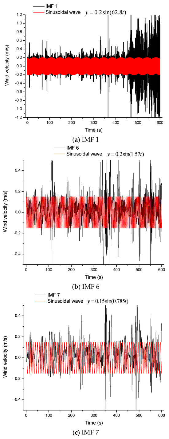
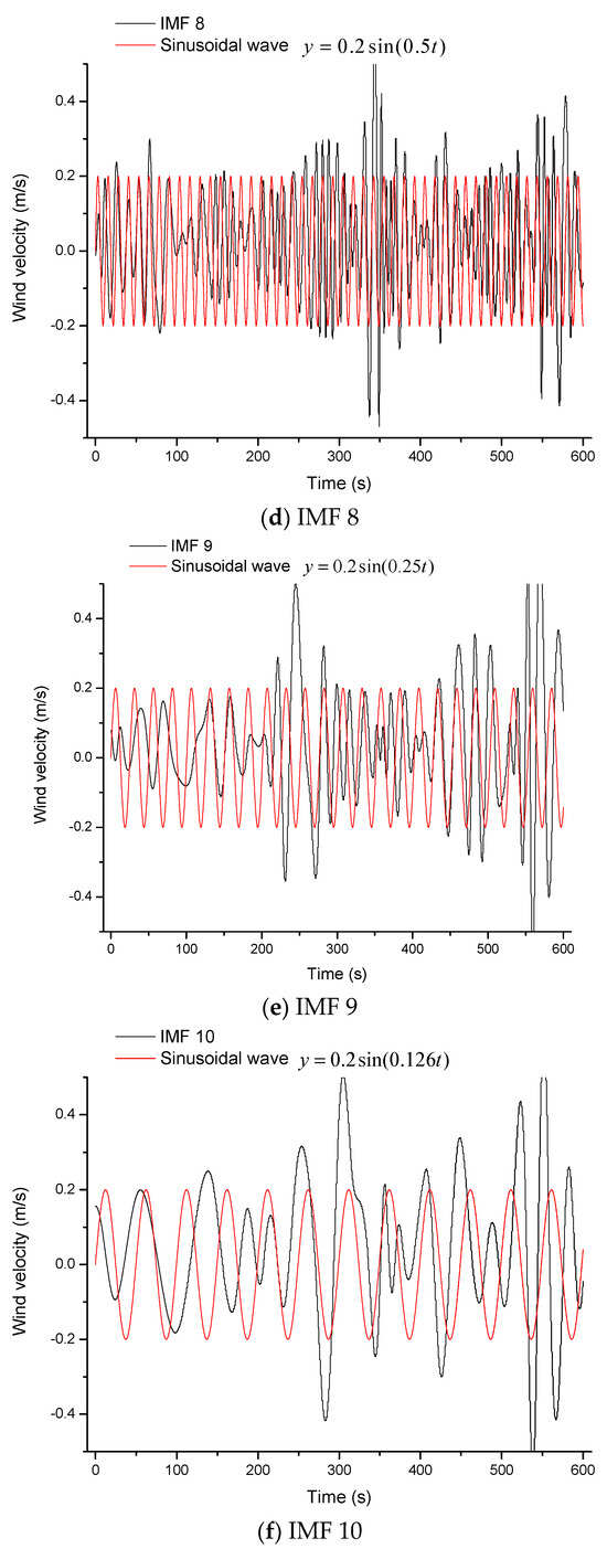
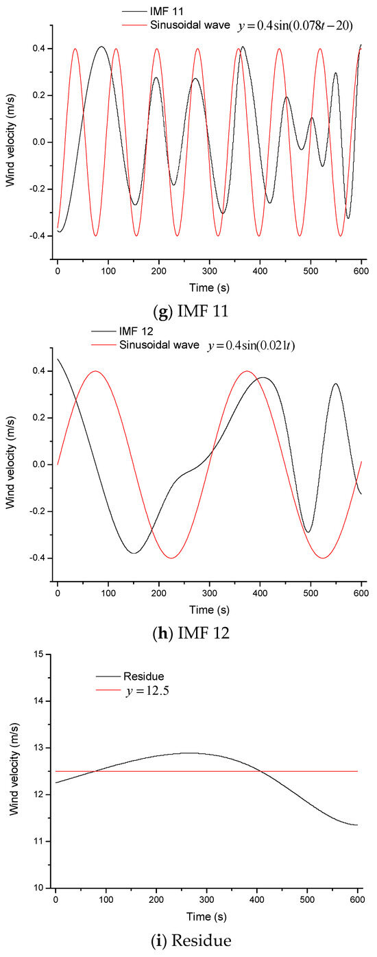
Figure 5.
IMFs and their approximate basic sinusoidal functions.
Table 2.
Amplitude, frequency, and phase of basic sinusoidal functions for all IMFs involved.

Figure 6.
Original non-stationary velocity sample and simulated senior sinusoidal function.
By inputting the inlet velocity sample varied according to the senior sinusoidal function obtained above to the program via the UDF operation, an approximate 2-D non-stationary flow event is simulated on the Fluent platform in accordance with the scenario measured on 29 November 2011 at the actual Pengcheng cooling tower site. A static circular object with a diameter of 1.6459 m is modeled in the numerical flow field to represent the throat section of Pengcheng tower. The inlet boundary condition is of the velocity-inlet type, and the outlet boundary conditions are of the pressure-outlet type. The wind field is assumed to be a compressible flow field and the k–ε standard viscous model is utilized. A standard wall function is adopted for the near-wall treatment. The pressure–velocity coupling equations are solved with the second-order implicit steady formulation. The residual is set to 0.001, and the time step is 0.05 s. It is assumed that the upcoming flow is laminar with negligible turbulence intensity for the numerical simulation.
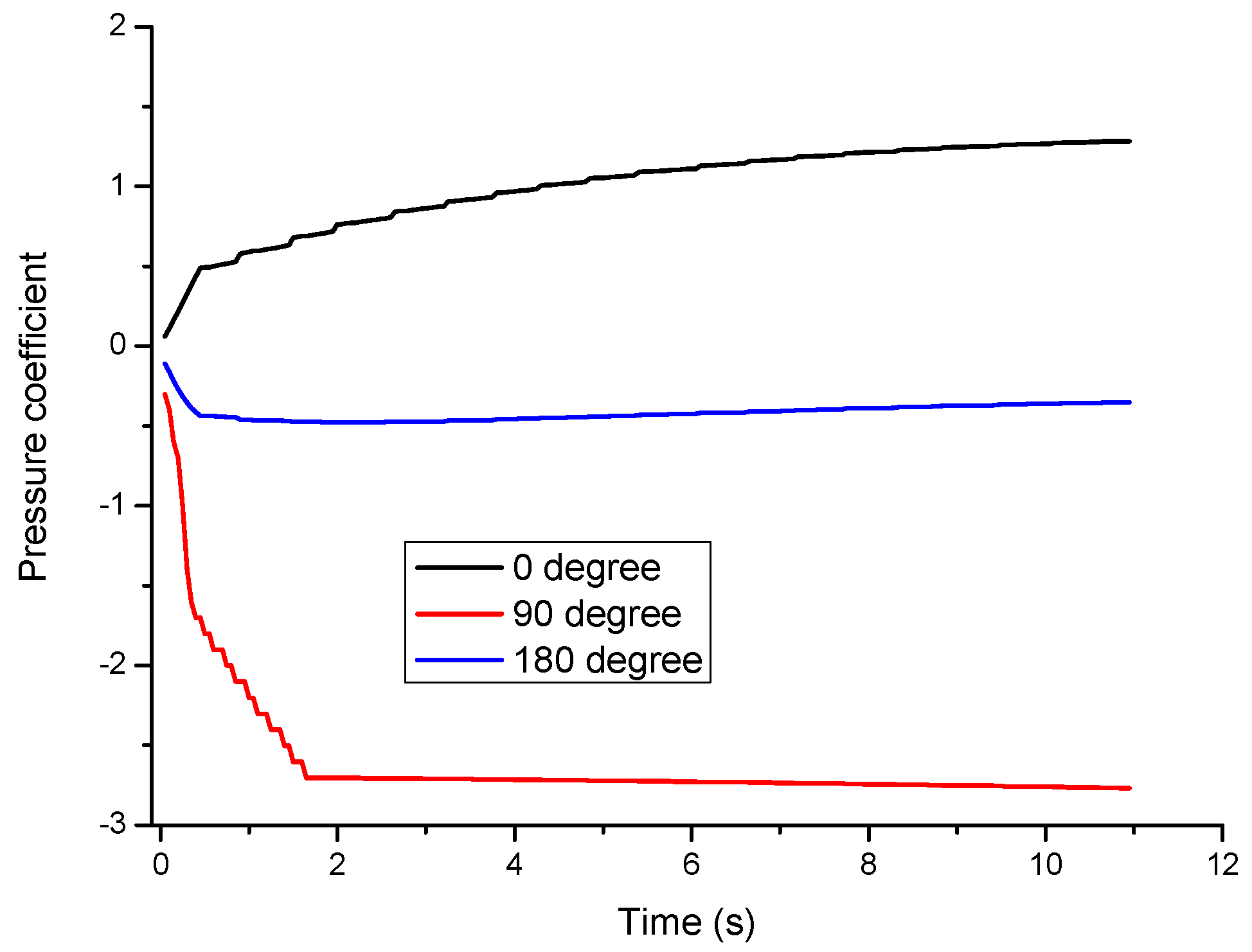
A calculated velocity contour is shown in Figure 7. As can be seen, the velocities calculated near the windward and the leeward regions are extremely low (≈0 m/s), and those calculated near the side regions are the highest (≈18 m/s). The velocities calculated at locations far from the circular object are close to the residue value (12.5 m/s). These observations agree well with the basic rules of flow physics. Moreover, three pressure coefficient samples calculated respectively at 0, 90, and 180 degrees on the circular object are shown in Figure 8. As shown, at the beginning of the duration (0–2 s), all the pressure coefficients dramatically change from the initial value (≈0) to the fixed values (1, −2.7, and −0.4 for 0, 90, and 180 degrees, respectively); during the remaining time, all the pressure coefficients stabilize at fixed values due to the stability of the flow pattern. Finally, we extracted all pressure coefficient samples calculated around a half of the surface of the circular object and processed the resulting values as the wind effects obtained in flow field B for our use.
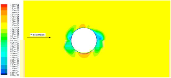
Figure 7.
Velocity contours obtained at end of duration (unit: m/s).
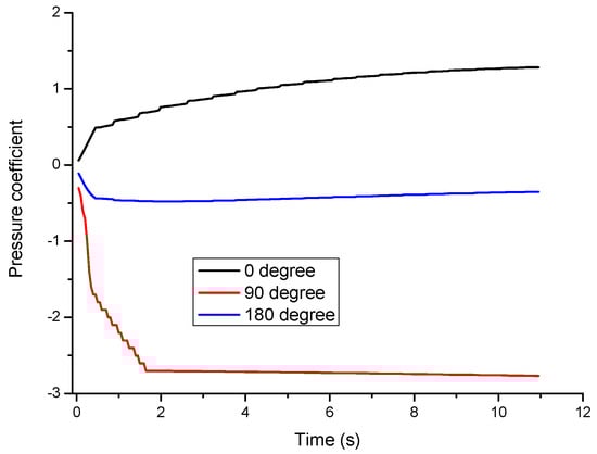
Figure 8.
Pressure coefficient time-histories calculated at 0, 90, and 180 degrees on the circular object.
3.3. Model Tests Conducted in TJ-3 Wind Tunnel
Two pressure measurement model tests are conducted in the TJ-3 passive wind tunnel of Tongji University, with flow fields simulated using the ABL empirical formulae listed in codes and monographs and the ABL wind velocity field measured on location, respectively. The flow field simulated using the ABL empirical formulae is regarded as the flow field for the traditional ABL wind tunnel model test, while the flow field simulated based on the ABL wind velocity field measured on location is regarded as flow field A. It should be emphasized that this simulation approach for flow field A employing a passive wind tunnel is different from the planned simulation method of utilizing a CFD platform or an actively controlled wind tunnel for the proposed research scheme (see Section 2) as the former is more economical and comparatively more effective.
The TJ-3 wind tunnel is a closed-circuit rectangular cross-section wind tunnel, wherein the size of the test section is 15 m in width, 2 m in height, and 14 m in length. The test wind speed can be continuously controlled in the 1.0 to 17.6 m/s range. The non-uniformity of the wind speed of the flow field in the test zone is less than 1%, the turbulence intensity is less than 0.5%, and the average flow deviation angle is less than 0.5°. Ref. [28] observes that the empirical turbulence intensity profile is noticeably greater than the field measurement data over the entire height. Therefore, the two flow fields mentioned above are simulated differently by adjusting the position and number of roughness elements and spires placed at the start of the wind tunnel work section (Figure 9a). After many attempts, both flow fields are simulated in the TJ-3 wind tunnel. Then, the pressure measurement model and the surroundings are modeled on a geometric scale of 1:200 using synthetic glass (see Figure 9b), and the pressure measurement tests are undertaken to measure wind effects on the tower model in the two flow fields.
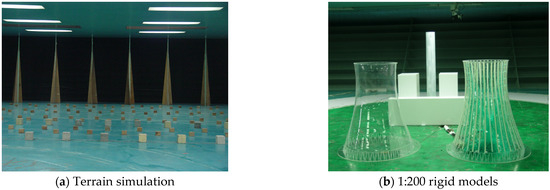
Figure 9.
Model test scenarios in TJ-3 wind tunnel.
The 36 × 12 taps are arranged on 12 vertical sections and in 36 horizontal circular directions for the pressure-measuring tower model. DSM3000 electronic pressure scanners of Scanivalve Corp. are used to obtain the wind pressures on the tower surfaces. The signal data are acquired at a sample rate of 312.5 Hz, and the sample length is 6000 data at one tap in each run. Without the aid of sufficient sticking paper belts along the vertical direction, the actual static characteristics of the prototype cooling tower at high Re are not simulated in the reduced-scale model. The turntable rotates from 0° to 360° at 22.5° intervals, but only the case with the same wind direction as that observed in the field on 29 November 2011 is considered, so the wind effects obtained from the model tests can compare with the full-scale results. The results obtained will be referred to as the data for the traditional ABL flow field and those for flow field A, respectively, for subsequent analyses.
3.4. Comparisons of Results
In this subsection of the study, we compared the wind loads obtained from full-scale measurements (Section 3.1), numerical simulation (Section 3.2), and passive model tests (Section 3.3) in accordance with the proposed research scheme. As depicted in Figure 10, the mean wind pressure distribution measured in the traditional ABL flow field closely resembles that measured in flow field A, with slight differences from the result measured in flow field B. However, all three distribution patterns are significantly smaller than the full-scale measurement data in the side region of flow separation (60–130 degrees).
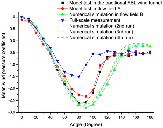
Figure 10.
Mean wind pressure distributions from full-scale measurement and model tests.
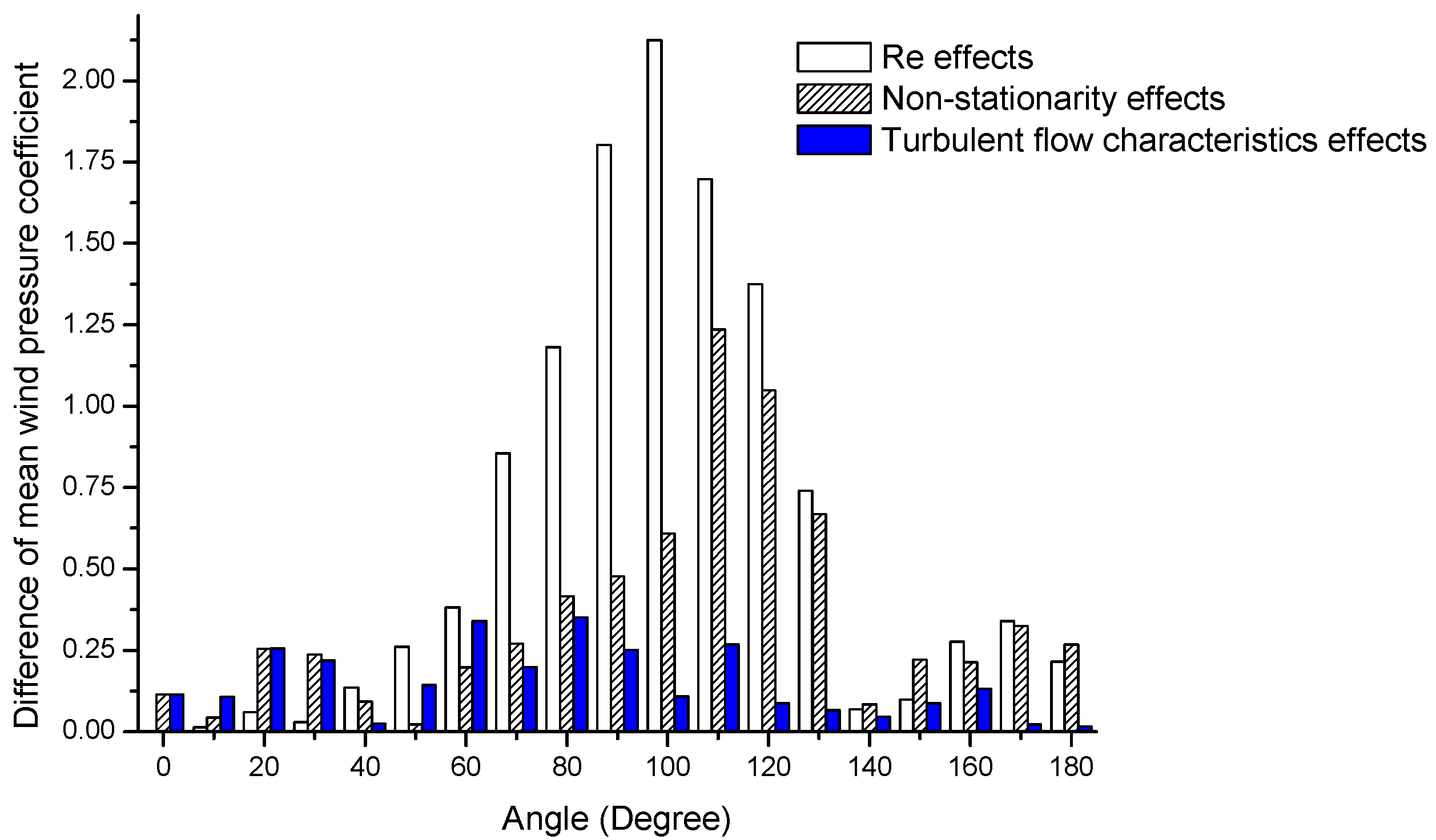
We used the data presented in Figure 10 to quantify and compare the three adverse effects, as shown in Figure 11. As seen from the figure, the Re effects obtained are extremely significant in the side region of flow separation and cannot be ignored. The non-stationarity effects are not as significant as Re effects but still carry significant weight in influencing wind loads. Finally, the turbulent flow characteristics effects are negligible around the half circle as it can be observed that all differences in the mean wind pressure coefficients are less than 0.4 for turbulent flow characteristics effects, but they are usually greater than 1.0 and 0.6 for Re effects and non-stationarity effects, respectively.
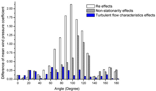
Figure 11.
Comparison of the three adverse effects.
It should be noted that the uncertainty is an important issue concerning all numerical simulations, and a significant source of uncertainty for CFD analyses is the initial state of calculation. Therefore, a simple quantitative estimate of the uncertainty from the numerical process presented in Section 3.2 is included in this portion of the study. By changing the initial phase () of all components in the original senior sinusoidal function (Equation (3)), three other senior sinusoidal functions are obtained as inlet velocity samples. By inputting these three inlet velocity samples into the numerical program, simulations are redone on the Fluent platform in flow field B, and the results for the three additional cases are added in Figure 10 (the three dashed lines). Comparing the results of the 2nd–4th runs of numerical analyses with the initial numerical data, it can be seen that they are basically close together, and the uncertainties in relative errors calculated are in the accepted range [0, 60%], suggesting that the uncertainty from the initial state of calculation is insignificant for the present study.
4. Method Conceived for Comparison Based on Model Tests
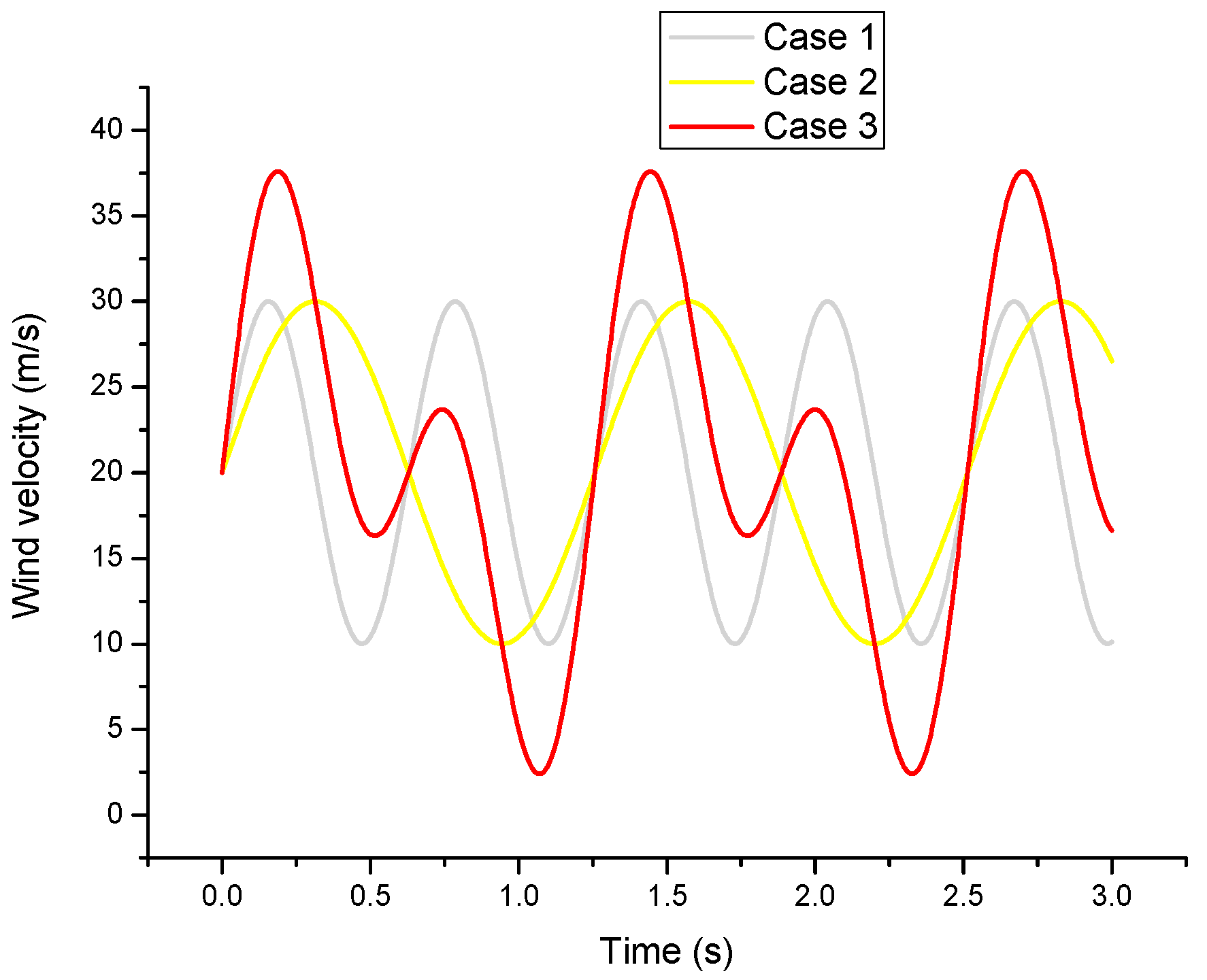
Our preliminary work in the TJ-6 wind tunnel indicated that simulating the original non-stationary ABL flow field or the senior sinusoidal flow field obtained by linearly superposing multiple basic sinusoidal waves as realized by the present numerical simulation (see Section 3.2) was difficult, but the individual flow fields with the input flow velocities varied according to the basic sinusoidal waves can be accurately simulated there. At present, a useful method should be conceived to facilitate the comparison based on the present experimental condition of TJ-6. To explore the relationships of wind effects on a circular cylinder obtained in multiple non-stationary sinusoidal wave flow fields, numerical analyses have been undertaken on a commercial CFD platform. Further, 2-D flows around a circular object with a diameter of 1.6459 m are simulated in three wind fields with the inlet velocities varied according to different sinusoidal functions. The inlet velocity time-histories for the three wind fields are shown in Figure 12. As can be seen, the velocity time-histories for Cases 1 and 2 are two different basic sinusoidal waves as they are of different periods; the velocity time-history for Case 3 is a senior sinusoidal wave obtained by linearly superposing the velocity time-histories of Cases 1 and 2. The inlet boundary condition is of the velocity-inlet type, and the outlet boundary conditions are of the pressure-outlet type. The wind field is assumed to be a compressible flow field and the k–ε standard viscous model is utilized. Compressibility means that the density is noticeably increased and the volume is thereby decreased for the fluid flow under pressure, and this effect should not be neglected for fluids like the wind in CFD simulations or analytical calculations. A standard wall function is adopted for the near-wall treatment. The pressure–velocity coupling equations are solved with the second-order implicit steady formulation. The residual is set to 0.001, and the time step is 0.05 s.
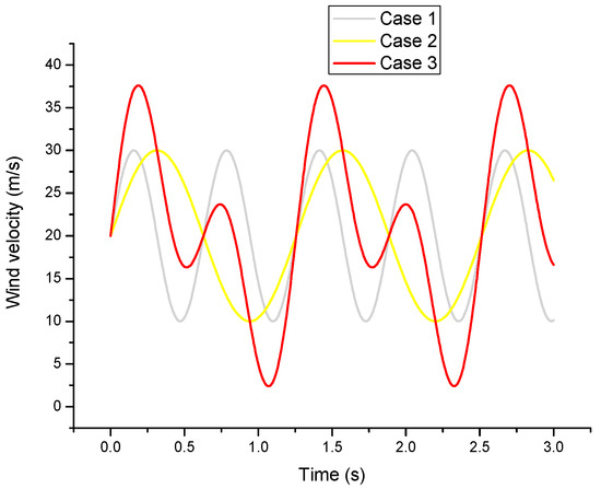
Figure 12.
Inlet velocity time-histories for the three wind fields.
After the numerical simulations, the wind loads on the circular object calculated for different cases are obtained and compared in Figure 13. As can be seen, the wind pressure coefficient time-histories calculated at different positions for all three cases are all non-stationary as they are all time-variant throughout the wind events. Moreover, the three samples for Cases 1–3 are noticeably different at the late stage of the wind events in Figure 13. The pressure coefficients for Case 2 are generally greater than those for Case 1 at different positions, and the pressure coefficients for Case 3 are in between them. Taking a step further, the averaged pressure coefficients of Cases 1 and 2 are added in Figure 13, and it is noted that the averaged values are close to the pressure coefficients for Case 3. Since the flow field for Case 3 is the linear superposition of those for Cases 1 and 2, it can be tentatively inferred from the above observations that wind effects measured in a comparatively more complicated flow field obtained by linearly superposing two basic sinusoidal wave flow fields are approximately equal to the averages of wind effects measured in the individual basic sinusoidal wave flow fields. To take advantage of this finding, we can simulate multiple non-stationary flow fields in the TJ-6 wind tunnel first, with the input flow velocities varied according to the basic sinusoidal waves obtained earlier to approximate the IMFs shown in Figure 5. Then, pressure measurements can be taken on a scaled Pengcheng cooling tower model in these non-stationary flow fields in the TJ-6 wind tunnel. Finally, the results obtained in multiple non-stationary flow fields (pressure coefficient samples) can be averaged as the wind effects obtained in flow field B for use to facilitate the new full-scale/model test comparison of wind effects on Pengcheng cooling tower. Finally, it can be observed that noticeable discontinuities can be observed on curves shown in Figure 13, and these should be caused by the noise, which is a significant proportion of the differences in the signals themselves. Our future works will focus on analyzing this uncertainty issue with the CFD simulation to enhance the validity of the presented comparisons.
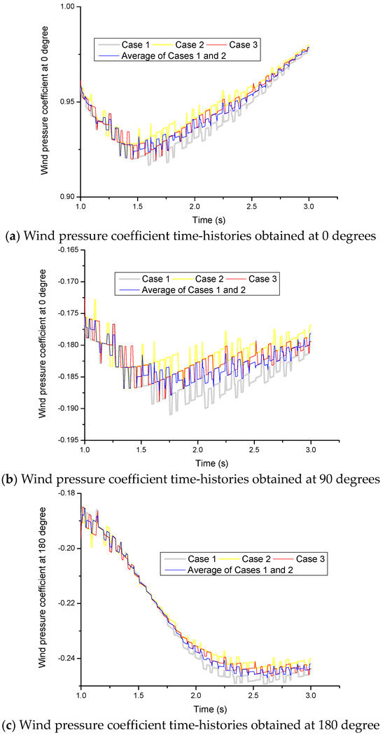
Figure 13.
Wind loads on the circular object calculated for different cases.
5. Conclusions
The main findings of this study, for a new research scheme for full-scale/model test wind effects comparisons based on a multiple-fan actively controlled wind tunnel technique, are summarized as follows:
- (1)
- In the wind engineering community, most full-scale/model test wind effects comparison studies only provide subjective explanations for observed differences without scientific validation. To address this issue, we have proposed a new research scheme that employs sinusoidal flow field simulations on a CFD platform or in a multiple-fan actively controlled wind tunnel for the full-scale/model test wind effects comparison for Pengcheng cooling tower. This technique allows us to separate mingled adverse effects and identify the most significant similarity problems with the traditional ABL wind tunnel technique for large cooling towers using quantitative data.
- (2)
- Multiple-fan actively controlled wind tunnels are well-known for their ability to simulate intricate non-stationary flow fields, and the literature indicates that the commercial CFD platforms can do the same. However, the preliminary works in the TJ-6 wind tunnel and on the Fluent platform indicated that simulating the original non-stationary ABL flow field was difficult. Instead, we found that flow fields with velocity inputs varied according to basic sinusoidal functions could be accurately simulated both in the TJ-6 wind tunnel and on the Fluent platform. Based on this observation, we adopted a new method to obtain wind effects on Pengcheng cooling tower in flow field B, which involved decomposing the original non-stationary velocity sample into multiple basic sinusoidal waves and numerically or physically simulating the sinusoidal wave flow fields. It should be admitted that the accuracy and the operability of the proposed approach for full-scale/model test comparisons of wind effects on Pengcheng cooling tower are not thoroughly demonstrated due to the limited numerical and physical research conditions. In the future, when the research conditions have been improved, we will undertake more systematic and meaningful works to further prove the effectiveness and efficiency of the proposed research scheme.
- (3)
- Based on our numerical case study of the Pengcheng cooling tower, our research indicates that Re effects are extremely significant, and non-stationarity effects cannot be ignored. However, we found via the present study that turbulent flow characteristics effects are negligible and do not significantly impact wind loads on the structure. This is a tentative conclusion since the present research is based on a single case of Pengcheng cooling tower merely using the CFD approach. Our future research will validate the correctness of this conclusion using more engineering backgrounds with various technical means.
Basically, two scientific issues have been addressed in the present manuscript: (1) how do the three adverse effects (Re effects, turbulent flow characteristics effects, and non-stationarity effects) contribute to the total difference between the full-scale measurement and the wind tunnel test?; (2) is the approach to reproduce the non-stationary flow field by superimposing the individual basic sinusoidal flow fields reliable? To answer the first question is the main object of the present research, and, to make it possible, the second scientific issue should be addressed in the situation that the research scheme proposed cannot be undertaken as planned on a commercial CFD platform or in a TJ-6 wind tunnel due to the incapability of both numerical and physical approaches in simulating the non-stationary flow field.
Finally, it should be noted that the uncertainty is an important issue perplexing the field measurements, the CFD simulations, and the wind tunnel tests in the field of wind engineering. With regard to field measurements, the uncertainties are usually associated with the nature of the realistic wind events (the unsteady and the non-stationary features), the testing errors related to the equipment and the human, and the free choice of the data processing practices. The causes of the uncertainties for wind tunnel tests are basically similar to those for field measurements, except that the unsteady and the non-stationary features are less significant for winds generated in the wind tunnel. In view of CFD simulations, although the uncertainty from the initial state of calculation is proven to be insignificant for the present study in Section 3.4, it should be noted that the fundamental uncertainties due to the unrealistic mathematical assumptions and simplifications adopted cannot be thoroughly eliminated, which are shown in the forms of free choices of the turbulence model, the wall function, the meshing, etc. Therefore, for the proposed research scheme for full-scale/model test comparisons of wind effects on Pengcheng cooling tower to work well, the uncertainties in simulations and experiments should be further estimated using probability theories or statistical approaches, such as the response surface method. Due to limited article length, these works will be undertaken and reported in the near future.
Author Contributions
Conceptualization, X.-X.C.; Methodology, L.Z.; Formal analysis, X.-X.C., B.-J.W. and Y.P.; Investigation, X.-X.C. and B.-J.W.; Supervision, Y.-J.G. and J.D. All authors have read and agreed to the published version of the manuscript.
Funding
This research was funded by National Natural Science Foundation of China (Grant No. 51908124) and the China Postdoctoral Science Foundation (Grant No. 2016M601793).
Data Availability Statement
The data presented in this study are available on request from the corresponding author.
Acknowledgments
The authors gratefully acknowledge the financial support from the National Natural Science Foundation of China (Grant No. 51908124) and the China Postdoctoral Science Foundation (Grant No. 2016M601793).
Conflicts of Interest
The authors declared no potential conflict of interest with respect to the research, authorship, and/or publication of this article.
References
- Huang, P.; Wang, X.; Gu, M. Field experiments for wind loads on a low-rise building with adjustable pitch. Int. J. Distrib. Sens. Netw. 2012, 8, 451879. [Google Scholar] [CrossRef]
- Tieleman, W.H. Problems associated with flow modelling procedures for low-rise structures. J. Wind Eng. Ind. Aerodyn. 1992, 41, 923–934. [Google Scholar] [CrossRef]
- Hoxey, R.P.; Robertson, A.P.; Richardson, G.M.; Short, J. Correction of wind-tunnel pressure coefficients for Reynolds number effect. J. Wind Eng. Ind. Aerodyn. 1997, 69, 547–555. [Google Scholar] [CrossRef]
- Richardson, G.M.; Hoxey, R.P.; Robertson, A.P.; Short, J. The Silsoe Building: Comparisons of pressures measured at full scale and in two wind tunnels. J. Wind Eng. Ind. Aerodyn. 1997, 72, 187–197. [Google Scholar] [CrossRef]
- Hoxey, R.P.; Reynolds, A.M.; Richardson, G.M.; Robertson, A.; Short, J. Observations of Reynolds number sensitivity in the separated flow region on a bluff body. J. Wind Eng. Ind. Aerodyn. 1998, 73, 231–249. [Google Scholar] [CrossRef]
- Liu, Z.; Prevatt, D.O.; Aponte-Bermudez, L.D.; Gurley, K.; Reinhold, T.; Akins, R. Field measurement and wind tunnel simulation of hurricane wind loads on a single family dwelling. Eng. Struct. 2009, 31, 2265–2274. [Google Scholar] [CrossRef]
- Dalgliesh, W.A. Comparison of model/full-scale wind pressures on a high-rise building. J. Ind. Aerodyn. 1975, 1, 55–66. [Google Scholar] [CrossRef]
- Dalgliesh, W.A. Comparison of model and full scale tests of the commerce court building in Toronto. In Proceedings of the International Workshop on Wind Tunnel Modeling Criteria and Techniques in Civil Engineering Applications, Gaithersburg, MD, USA, 14–16 April 1982. [Google Scholar]
- Li, Q.S.; Xiao, Y.Q.; Wong, C.K. Full-scale monitoring of typhoon effects on super tall buildings. J. Fluids Struct. 2005, 20, 697–717. [Google Scholar] [CrossRef]
- Li, Q.S.; Xiao, Y.Q.; Fu, J.Y.; Li, Z. Full-scale measurements of wind effects on the Jin Mao building. J. Wind Eng. Ind. Aerodyn. 2007, 95, 445–466. [Google Scholar] [CrossRef]
- Li, Q.S.; Xiao, Y.Q.; Wu, J.R.; Fu, J.; Li, Z. Typhoon effects on super-tall buildings. J. Sound Vib. 2008, 313, 581–602. [Google Scholar] [CrossRef]
- Fu, J.Y.; Li, Q.S.; Wu, J.R.; Xiao, Y.; Song, L. Field measurements of boundary layer wind characteristics and wind-induced responses of super-tall buildings. J. Wind Eng. Ind. Aerodyn. 2008, 96, 1332–1358. [Google Scholar] [CrossRef]
- Fu, J.Y.; Wu, J.R.; Xu, A.; Li, Q.; Xiao, Y. Full-scale measurements of wind effects on Guangzhou West Tower. Eng. Struct. 2012, 35, 120–139. [Google Scholar] [CrossRef]
- Frandsen, J.B. Simultaneous pressures and accelerations measured full-scale on the Great Belt East suspension bridge. J. Wind Eng. Ind. Aerodyn. 2001, 89, 95–129. [Google Scholar] [CrossRef]
- Li, H.; Laima, S.; Zhang, Q.; Li, N.; Liu, Z. Field monitoring and validation of vortex-induced vibrations of a long-span suspension bridge. J. Wind Eng. Ind. Aerodyn. 2014, 124, 54–67. [Google Scholar] [CrossRef]
- Pirner, M. Wind pressure fluctuations on a cooling tower. J. Wind Eng. Ind. Aerodyn. 1982, 10, 343–360. [Google Scholar] [CrossRef]
- Cheng, X.X.; Dong, J.; Peng, Y.; Zhao, L.; Ge, Y.J. A study of non-stationary wind effects on a full-scale large cooling tower using empirical mode decomposition. Math. Probl. Eng. 2017, 2017, 9083426. [Google Scholar] [CrossRef]
- Geurts, C.P.W. Full-scale and wind-tunnel measurements of the wind and wind-induced pressures over suburban terrain. J. Wind Eng. Ind. Aerodyn. 1996, 64, 89–100. [Google Scholar] [CrossRef]
- Richards, P.J.; Hoxey, R.P.; Short, L.J. Wind pressures on a 6m cube. J. Wind Eng. Ind. Aerodyn. 2001, 89, 1553–1564. [Google Scholar] [CrossRef]
- Chen, B.; Wu, T.; Yang, Y.; Yang, Q.; Li, Q.; Kareem, A. Wind effects on a cable-suspended roof: Full-scale measurements and wind tunnel based predictions. J. Wind Eng. Ind. Aerodyn. 2016, 155, 159–173. [Google Scholar] [CrossRef]
- Dalgliesh, W.A. Experience with wind pressure measurements on a full-scale building. In Proceedings of the Technical Meeting Concerning Wind Loads on Buildings and Structures, Gaithersburg, MD, USA, 27–28 January 1969. [Google Scholar]
- Jia, J.P.; He, X.Q.; Jin, Y.J. Statistics, 4th ed.; China Renmin University Press: Beijing, China, 2009. (In Chinese) [Google Scholar]
- Dong, K.H. Evaluation of the non-stationary wind and its effect on structural wind loads. Master’s Thesis, Beijing Jiaotong Univeristy, Beijing, China, 2015. (In Chinese). [Google Scholar] [CrossRef]
- Cao, S.; Nishi, A.; Kikugawa, H.; Matsuda, Y. Reproduction of wind velocity history in a multiple fan wind tunnel. J. Wind Eng. Ind. Aerodyn. 2002, 90, 1719–1729. [Google Scholar] [CrossRef]
- Nishi, A.; Kikugawa, H.; Matsuda, Y.; Tashiro, D. Turbulence control in multiple-fan wind tunnels. J. Wind Eng. Ind. Aerodyn. 1997, 67, 861–872. [Google Scholar] [CrossRef]
- Cheng, X.X.; Zhao, L.; Ge, Y.J.; Wu, G. Wind effects on large cooling tower in velocity fields of different non-stationary levels. Proc. Inst. Civ. Eng.-Struct. Build. 2023, 176, 630–645. [Google Scholar] [CrossRef]
- Yang, Y.; Li, M.; Ma, C.; Li, S. Experimental investigation on the unsteady lift of an airfoil in a sinusoidal streamwise gust. Phys. Fluids 2017, 29, 051703. [Google Scholar] [CrossRef]
- Cheng, X.X.; Zhao, L.; Ke, S.T.; Ge, Y.-J. A New Research Scheme for Full-Scale/Model Test Comparisons to Validate the Traditional Wind Tunnel Pressure Measurement Technique. Appl. Sci. 2022, 12, 12847. [Google Scholar] [CrossRef]


Disclaimer/Publisher’s Note: The statements, opinions and data contained in all publications are solely those of the individual author(s) and contributor(s) and not of MDPI and/or the editor(s). MDPI and/or the editor(s) disclaim responsibility for any injury to people or property resulting from any ideas, methods, instructions or products referred to in the content. |
© 2023 by the authors. Licensee MDPI, Basel, Switzerland. This article is an open access article distributed under the terms and conditions of the Creative Commons Attribution (CC BY) license (https://creativecommons.org/licenses/by/4.0/).