Finding the Exact Radiative Field of Triangular Sources: Application for More Effective Shading Devices and Windows

Featured Application

Design and construction of innovative shading devices and fins.

Abstract

Triangles are an ever-present feature in nature, which the building construction industry duly echoes. However, an exact expression intended to supply the radiant field of any triangle in an upright or inclined position has not been identified by previous research. In this case, the author has been able to solve, via direct integration, the canonical expression of radiative transfer. This result alone confers a myriad of possibilities, that had been inconceivable before, for studying in detail the three-dimensional heat-transfer behavior of volumes and figures in which triangles manifest, such as fins, windows, roof-gables and louvers of various kinds. Typically, shading devices, when tilted, give rise in their extremes to rhomboidal shapes which were difficult to take into account or had to be subject to discretization and subsequent Monte Carlo methods in order to perform an approximate calculation of their emissions. This implied a lengthy and inexact procedure that induced many errors and consumed computing time. We can now avoid all these former downsides due to the advances hereby presented. As this novel expression can be converted into an algorithm, it will be advantageously employed for simulation. This significant finding dovetails into the intricate puzzle of radiated heat and we believe that its consequences will greatly affect the conception and design of HVAC devices, aircraft manufacturing and specifically the building or lighting industries, among others.

1. Introduction

It is known that form factors are a substantial entity in all the phenomena that concern radiation. As this powerful and subtle kind of heat transfer does not imply any sort of proximity between the involved elements, sheer form and a geometric approach become paramount for the distribution of energies [1]. However, the diffusion of radiative fields is heavily dependent on the spatial configuration of surface sources [2]. At the level of unit areas of no defined shape, the issue may seem nugatory [3,4]; but when we arrive at definite widespread forms like the circle or the triangle, it is frequently problematic to extend these well-known differential equations to concrete and finite forms arbitrarily displayed, as we need to manage two sets of different and often complex double integrals [4]. It is evident that, to achieve a manageable solution from quadruple integrands even of the most basic emitters implies a feat of calculus unsuitable for conventional engineering [5], but it is substantially needed to ascertain the energy balance achieved in the said elements.

Even recent studies have failed to overcome this severe hindrance in the completion of important problems in radiative transfer [6,7]. Experts have too long resorted to numerical or statistical approaches like probabilistic methods [8], albeit that they are inconsequential in most cases, not merely due to the many errors that arise in the lengthy process but also due to the unfeasibility of proving their results, as they remained the sole procedure available to attempt to overcome such problems.

In this case, the author has followed a special procedure of dummy variables to perform the inner part of the integral, that is referred to the receiving source in an exact manner. Formerly, only rectangles and parallel disks could have been submitted to total integration [7]. It is paradoxical that the relatively simple form of the triangle could not have been included in the catalog of solved form factors but we have to admit that some mathematical drawbacks impeded it for an undesirably long lapse of time [9].

In this manner, the problem can be prepared for the final phase of integration as the dummy variables now take an active value in the third and fourth round of operation that is usually performed by numerical methods [10]. We have to bear in mind that, in the early part, the more feasible equation due only to the so-called configuration factor (an equation that reduces the interchange to arbitrary points on the emitting surface) is treated and solved [8]. A considerable fraction of the difficulty of the problem lies in the three-dimensional nature of the elements under consideration [11].

Different approximations so far employed for the problem have shown increasing flaws [12], as, being an elementary unit in itself, the triangle is not apt for division into (let us say) square or round tiles, for example. The accurate finding of such expressions can be considered a postulate in itself, that can be added rightfully to the six principles of radiation exchanges that we have developed previously [13]. Such algebraic expressions can be automatically computed with the software that we have created and a detailed explanation of the procedure segues out.

2. Materials and Methods: General Flux Expression

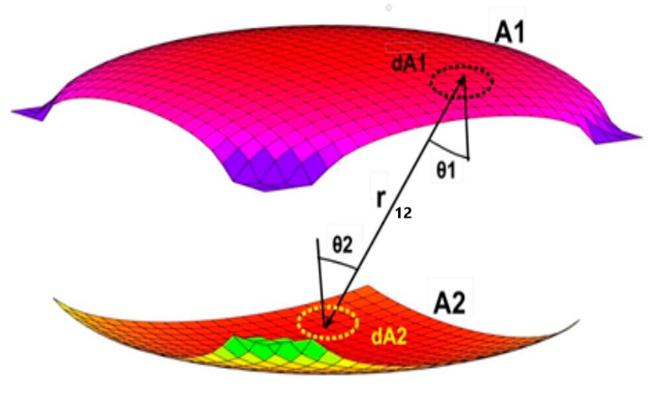
As has been enunciated several times since the last quarter of the 18th century [14], the most general expression that defines the probability of an arbitrary interchange of radiated flux for any kind of three-dimensional form positioned in the manner illustrated in Figure 1, follows the structure described as follows (Equation (1)):

$$d{\varphi }_{12}=\left(E_1-E_2\right)\cos {\theta }_1\cos {\theta }_2\frac{d{A}_{1}d{A}_2}{\pi r_{12}^2}$$

(1)

Equation (1) initiates in the reciprocal principle, originally enunciated by J. H. Lambert [15,16,17] and it yields the probable amount of radiation emitted by unit area that is transferred (W/m²), from each surface defined as scalar quantities E₁ and E₂. The respective angles θ₁ and θ₂ that appear in the figure represent the deviation from the perpendicular that the vector r_ij encounters in its rectilinear way from a random point in surface 1 to its correspondent in surface 2 [18].

The solution of Equation (1), which renders the value of the form factor between the two surfaces, would normally involve four rounds of integration, following Equation (2) [15].

$$F_{ij}=\frac{1}{A_i}{\int }_{A_i}^{}{\int }_{A_j}^{}\cos {\theta }_i\cos {\theta }_j\frac{d{A}_{i}d{A}_j}{\pi r_{ij}^2}$$

(2)

However, we have concentrated in this article on the first two stages (Equation (3)), which are also simpler, leaving a sort of harbinger for the next step, which is a variable (x₀) that can be considered a constant (dummy) in these early phases and will only become active for the third and fourth rounds of integrals.

$$f_{d{A}_i-A_j}={\int }_{A_j}^{}\frac{\cos {\theta }_i\cos {\theta }_j}{\pi r_{ij}^2}d{A}_j$$

(3)

The latter operation is usually performed by means of deterministic numerical methods through an extension of the results to the whole emitting surface. With it, we can obtain the value of the form factor for the two complete surfaces in a more comfortable and accurate manner [18]. Ensuingly, we can use these form factors in various three-dimensional volumes that appear in most shading devices, some kinds of buildings affected by triangles, like warehouses and gabled-ceiling spaces, and different industrial and aeronautical fixtures [19,20].

For other different positions of the surface sources, an exact solution has not been achieved yet [5], nor for irregular fragments of triangles, rectangles and circles or even for the familiar form of the sphere [20,21].

Intermediate steps to proceed only with the first and the second round of integration have been proposed [22]. They usually end at a particular point or elementary area that pertains to the receiving surface. Some of these are recorded under the inexact and cumbersome manner of copied nomograms for catalogs of radiation view factors [23,24]. Such results are somewhat indicative but they are by no means general and can be misleading in many situations.

In order to proceed with the said method, we shall start with a general right triangle of sides a (vertical) and b (horizontal) located at the origin of coordinates (Figure 2).

Under this disposition, the coordinate Z axis is vertical and X is horizontal and perpendicular, the sides of the triangle are, in Z, equal to a, and, in X, to b, as seen in Figure 2.

The tangent of the angle formed from the upper edge of the triangle to the horizontal equates tanα = a/b, therefore, the equation of the superior line of the triangle is,

z = (a/b)x

The axis Y in the graph represents the free coordinate perpendicular to X.

Introducing the “dummy” variable x₀, the squared distance (Equation (5)) from one receiving point-source of the triangle to another emitting point moving freely over the plane XY, presented as r₁₂ in Equation (2) above, would be:

$$r_{12}^2={\left(x-x_0\right)}^2+y^2+z^2$$

(4)

The respective cosines β and γ, to the normal from Equations (1)–(3), would be accordingly y/r₁₂ and z/r₁₂.

The integral to solve deriving from Equation (3), would then turn to (Equation (6)):

$$f_{d{A}_i-A_j}=I=\frac{1}{\pi }{\int }_0^b{\int }_0^{\frac{a}{b}x}\frac{yzdzdx}{{\left[{\left(x-x_0\right)}^2+y^2+z^2\right]}^2}$$

(5)

We need to solve the root equation for a generality of types of triangles in diverse positions [25]. To avoid special difficulties, we will provide the solution at the intermediate stage of configuration, that is, the double integral firstly, obtained point by point over a rectangular emitting field. Once we have achieved this, to advance towards the complete form factor of Equation (2), we need to apply another property previously enunciated by the author [26]; namely the form factor is the average over the emitting surface of the configuration factor previously obtained on a point basis. It is now feasible by numerical calculus alone to extract such a mean value for any kind of planar figures contained in the said field. With a similar approach, the total form factors are found for the usual sets of precincts, such as prisms or oblique cuboids. Inter-reflection within the so-generated space is also an issue that we have to foresee; in the case of triangular prisms, we would require a set of five equations with five unknowns, which is detailed in the Appendix A [27].

For example, when designing and solving inclined slats, the triangles that appear are not right, but usually they appear as obtuse or acute; in these situations, we cannot employ the already solved form factor for perpendicular rectangles; instead we need to resort to the extended formulas developed by the author [28] to take into account the exchanges between inclined rectangles.

3. Results: Solutions for Various Forms of Triangles and Trapezes

3.1. Right Triangle with Minor Vertex at the Origin of Coordinates

Consequently, let us advance towards the solution set out above for the more representative triangles and rhomboids, beginning with the case depicted in Figure 3.

In Equation (6), we mentioned the integral to be solved as,

$$f_{12}=\frac{1}{\pi }{\int }_0^b{\int }_0^{\frac{a}{b}x}\frac{yzdzdx}{{\left[{\left(x-x_0\right)}^2+y^2+z^2\right]}^2}$$

(6)

In this case, the primitive is the quotient of the denominator and integration with respect to z gives,

$${\int }_0^{\frac{a}{b}x}\frac{yzdz}{{\left[{\left(x-x_0\right)}^2+y^2+z^2\right]}^2}=-\frac{y}{2}{\left[\frac{1}{{\left(x-x_0\right)}^2+y^2+z^2}\right]}_0^{\frac{a}{b}x}$$

(7)

Substituting, it yields,

$$=-\frac{y}{2}{\left[\frac{1}{{\left(x-x_0\right)}^2+y^2+z^2}\right]}_0^{\frac{a}{b}x}=\frac{y}{2}\left(\frac{1}{{\left(x-x_0\right)}^2+y^2}-\frac{1}{{\left(x-x_0\right)}^2+y^2+\frac{a^2}{b^2}{x}^2}\right)$$

(8)

And regrouping, the result is

$$\frac{y}{2}\left(\frac{1}{{\left(x-x_0\right)}^2+y^2}-\frac{b^2}{{{a^{2}x}^2+b^2\left(x-x_0\right)}^2+{b^{2}y}^2}\right)$$

(9)

Now, we only need to integrate with respect to x.

The first part presents not much difficulty to identify,

$${\int }_0^b\frac{dx}{{\left(x-x_0\right)}^2+y^2}=\frac{1}{y}\left[arctan\frac{x_0}{y}+arctan\frac{b-x_0}{y}\right]$$

(10)

The second part is slightly lengthier in calculation,

$$\begin{gathered} {\int }_0^b\frac{b^{2}dx}{{{a^{2}x}^2+b^2\left(x-x_0\right)}^2+{b^{2}y}^2} \\ =\frac{b}{\sqrt{{a^{2}x}_0^2+y^2\left(a^2+b^2\right)}}{\left[arctan\frac{x\left(a^2+b^2\right)-x_0{b}^2}{b\sqrt{{a^{2}x}_0^2+y^2\left(a^2+b^2\right)}}\right]}_0^b \\ =\frac{b}{\sqrt{{a^{2}x}_0^2+y^2\left(a^2+b^2\right)}}\left[arctan\frac{a^2+b^2-x_{0}b}{\sqrt{{a^{2}x}_0^2+y^2\left(a^2+b^2\right)}} \\ +arctan\frac{x_{0}b}{\sqrt{{a^{2}x}_0^2+y^2\left(a^2+b^2\right)}}\right] \end{gathered}$$

(11)

Arranging the two parts and multiplying by y/2, which was outside of the integral in Equation (8), we obtain:

$$\begin{gathered} \frac{1}{2}\left(\left[arctan\frac{x_0}{y}+arctan\frac{b-x_0}{y}\right] \\ -\frac{by}{\sqrt{{a^{2}x}_0^2+y^2\left(a^2+b^2\right)}}\left[arctan\frac{a^2+b^2-x_{0}b}{\sqrt{{a^{2}x}_0^2+y^2\left(a^2+b^2\right)}} \\ +arctan\frac{x_{0}b}{\sqrt{{a^{2}x}_0^2+y^2\left(a^2+b^2\right)}}\right]\right) \end{gathered}$$

(12)

Finally, we need to divide everything by π to keep the factor dimensionless in terms of radiant power,

$$\begin{gathered} f_{21}=\frac{1}{2\pi }\left(\left(arctan\frac{b-x_0}{y}+arctan\frac{x_0}{y}\right) \\ -\frac{by}{\sqrt{{a^{2}x}_0^2+y^2\left(a^2+b^2\right)}}\left(arctan\frac{a^2+b^2-x_{0}b}{\sqrt{{a^{2}x}_0^2+y^2\left(a^2+b^2\right)}} \\ +arctan\frac{x_{0}b}{\sqrt{{a^{2}x}_0^2+y^2\left(a^2+b^2\right)}}\right)\right) \end{gathered}$$

(13)

If x₀ = 0, which means that we are calculating at the vertex point of the triangle,

$$\begin{gathered} f_{21}=\frac{1}{2\pi }\left(\left(arctan\frac{b}{y}\right)-\frac{by}{\sqrt{y^2\left(a^2+b^2\right)}}\left(arctan\frac{a^2+b^2}{\sqrt{y^2\left(a^2+b^2\right)}}\right)\right)=\frac{1}{2\pi }\left(\left(arctan\frac{b}{y}\right) \\ -\frac{b}{\sqrt{a^2+b^2}}\left(arctan\frac{a^2+b^2}{y\sqrt{a^2+b^2}}\right)\right) \end{gathered}$$

(14)

This was obtained previously by the author for the triangle at its minor vertex [5],

$$f_{12}=\frac{1}{2\pi }\left[arctan\frac{b}{y}-\frac{b}{\sqrt{a^2+b^2}}arctan\frac{a^2+b^2}{y\sqrt{a^2+b^2}}\right]$$

(15)

If x₀ = b, the end of the base, then,

$$f_{21}=\frac{1}{2\pi }\left(arctan\frac{b}{y}-\frac{by}{\sqrt{{a^{2}b}_{}^2+y^2\left(a^2+b^2\right)}}\left(arctan\frac{a^2}{\sqrt{{a^{2}b}_{}^2+y^2\left(a^2+b^2\right)}}+arctan\frac{b^2}{\sqrt{a^2{b}^2+y^2\left(a^2+b^2\right)}}\right)\right)$$

(16)

This was the formula previously obtained for the horizontal extreme corresponding to the right angle, which coincides exactly with the former, (Equation (17)) [29].

$$f_{12}=\frac{1}{2\pi }\left(\left[arctan\frac{b}{y}\right]-\frac{by}{\sqrt{a^2{b}^2+y^2\left(a^2+b^2\right)}}\left[arctan\frac{b^2}{\sqrt{a^2{b}^2+y^2\left(a^2+b^2\right)}}+arctan\frac{a^2}{\sqrt{a^2{b}^2+y^2\left(a^2+b^2\right)}}\right]\right)$$

(17)

Finally, if we make x₀ = x, igniting the dummy variable, the above expression compares well with the one used for the rectangle of vertical side a and horizontal side b when the study point moves freely on the horizontal plane (Equation (18)) [7].

$$f_{21}=\frac{1}{2\pi }\left(arctan\frac{b-x}{y}+arctan\frac{x}{y}-\frac{y}{\sqrt{a^2+y^2}}\left(arctan\frac{b-x}{\sqrt{a^2+y^2}}+arctan\frac{x}{\sqrt{a^2+y^2}}\right)\right)$$

(18)

Let us now calculate, for the sake of generality, the same triangle in a more general position outside the origin of coordinates, see Figure 4.

In this case, integration limits in z, would change between,

$$\begin{gathered} z=\frac{a}{b}x-\frac{am}{b}\text{and z = 0} \\ {\int }_0^{\frac{a}{b}x-\frac{am}{b}}\frac{yzdz}{{\left[{\left(x-x_0\right)}^2+y^2+z^2\right]}^2}=-\frac{y}{2}{\left[\frac{1}{{\left(x-x_0\right)}^2+y^2+z^2}\right]}_0^{\frac{a}{b}x-\frac{am}{b}} \\ =-\frac{y}{2}{\left[\frac{1}{{\left(x-x_0\right)}^2+y^2+z^2}\right]}_0^{\frac{a}{b}x-\frac{am}{b}}=\frac{y}{2}\left(\frac{1}{{\left(x-x_0\right)}^2+y^2}-\frac{1}{{\left(x-x_0\right)}^2+y^2+{\left(\frac{a}{b}x-\frac{am}{b}\right)}^2}\right) \end{gathered}$$

(19)

But

$${\left(\frac{a}{b}x-\frac{am}{b}\right)}^2={\frac{a^2}{b^2}{x}^2-2\frac{a^2}{b^2}mx}^{}-\frac{a^2{m}^2}{b^2}=\frac{a^2}{b^2}(x^2-2mx+m^2)$$

(20)

And regrouping, the partial result is

$$\frac{y}{2}\left(\frac{1}{{\left(x-x_0\right)}^2+y^2}-\frac{1}{{\left(x-x_0\right)}^2+y^2+\frac{a^2(x^2-2mx+m^2)}{b^2}}\right)$$

(21)

Conveniently developed, this gives,

$$\frac{y}{2}\left(\frac{1}{{\left(x-x_0\right)}^2+y^2}-\frac{b^2}{b^2{\left(x-x_0\right)}^2+{b^{2}y}^2+a^2{x}^2-2a^{2}mx+a^2{m}^2}\right)$$

(22)

That is,

$$\frac{y}{2}\left(\frac{1}{{\left(x-x_0\right)}^2+y^2}-\frac{b^2}{b^2{\left(x-x_0\right)}^2+{b^{2}y}^2+a^2(x^2-2mx+m^2)}\right)$$

(23)

The first term of the integral is already solved in Equation (10),

$${\int }_m^{b+m}\frac{dx}{{\left(x-x_0\right)}^2+y^2}=\frac{1}{y}\left[arctan\frac{b+m-x_0}{y}+arctan\frac{x_0-m}{y}\right]$$

(24)

For the second part, we need to integrate,

$${\int }_m^{b+m}\frac{b^{2}dx}{b^2{\left(x-x_0\right)}^2+{b^{2}y}^2+a^2(x^2-2mx+m^2)}$$

(25)

Developing all the terms in the denominator, we receive,

$$b^2{\left(x-x_0\right)}^2+{b^{2}y}^2+a^2\left(x^2-2mx+m^2\right)=b^2\left(x^2+{x_0}^2-2x{x}_0\right)+{b^{2}y}^2+a^2{x}^2-2a^{2}mx+a^2{m}^2$$

(26)

And grouping in terms of x,

$${(a}^2+b^2)x^2-2\left(b^2{x}_0+a^{2}m\right)x+b^2\left(y^2+{x_0}^2\right)+a^2{m}^2$$

(27)

The final integral to be solved is,

$$\begin{gathered} {\int }_m^{b+m}\frac{b^{2}dx}{{(a}^2+b^2)x^2-2\left(b^2{x}_0+a^{2}m\right)x+b^2\left(y^2+{x_0}^2\right)+a^2{m}^2}= \\ =\frac{2b^2}{b\sqrt{{a^2(y^2+(x_0-m)}_{}^2)+{b^{2}y}^2}}{\left[arctan\frac{2x\left(a^2+b^2\right)-2(a^{2}m+b^2{x}_0)}{2b\sqrt{{a^2(y^2+(x_0-m)}_{}^2)+b^2{y}^2}}\right]}_m^{b+m} \\ =\frac{2b}{\sqrt{{a^2\left(x_0-m\right)}_{}^2+y^2\left(a^2+b^2\right)}}\left[arctan\frac{b(a^2+b\left(b+m-x_0\right))}{b\sqrt{{a^2\left(x_0-m\right)}_{}^2+y^2\left(b^2+a^2\right)}} \\ -arctan\frac{b^2(m-x_{0)}}{b\sqrt{{a^2\left(x_0-m\right)}_{}^2+y^2\left(b^2+a^2\right)}}\right] \end{gathered}$$

(28)

$$\begin{gathered} =\frac{2b}{\sqrt{{a^2\left(x_0-m\right)}_{}^2+y^2\left(a^2+b^2\right)}}\left[arctan\frac{a^2+b\left(b+m-x_0\right)}{\sqrt{{a^2\left(x_0-m\right)}_{}^2+y^2\left(a^2+b^2\right)}} \\ -arctan\frac{b(m-x_{0)}}{\sqrt{{a^2\left(x_0-m\right)}_{}^2+y^2\left(a^2+b^2\right)}}\right] \end{gathered}$$

(29)

Arranging all the necessary terms and multiplying by y/2, we obtain,

$$\begin{gathered} f_{21}=\frac{1}{2\pi }\left[arctan\frac{b+m-x_0}{y}+arctan\frac{x_0-m}{y}\right] \\ -\frac{by}{\sqrt{{a^2\left(x_0-m\right)}_{}^2+y^2\left(a^2+b^2\right)}}\left[arctan\frac{a^2+b\left(b+m-x_0\right)}{\sqrt{{a^2\left(x_0-m\right)}_{}^2+y^2\left(a^2+b^2\right)}} \\ -arctan\frac{b(m-x_{0)}}{\sqrt{{a^2\left(x_0-m\right)}_{}^2+y^2\left(a^2+b^2\right)}}\right] \end{gathered}$$

(30)

By making m = 0, we would find that,

$$\begin{gathered} f_{21}=\frac{1}{2\pi }\left[arctan\frac{b-x_0}{y}+arctan\frac{x_0}{y}\right] \\ -\frac{by}{\sqrt{a^2{x}_0^2+y^2\left(a^2+b^2\right)}}\left[arctan\frac{a^2+b^2-b{x}_0}{\sqrt{a^2{x}_0^2+y^2\left(a^2+b^2\right)}} \\ +arctan\frac{b{x}_0}{\sqrt{a^2{x}_0^2+y^2\left(a^2+b^2\right)}}\right] \end{gathered}$$

(31)

This is exactly the same as previously found in Equation (13), which we now define as the Cabeza-Lainez seventh postulate, that is,

$$\begin{gathered} f_{21}=\frac{1}{2\pi }\left(\left(arctan\frac{b-x_0}{y}+arctan\frac{x_0}{y}\right) \\ -\frac{by}{\sqrt{{a^{2}x}_0^2+y^2\left(a^2+b^2\right)}}\left(arctan\frac{a^2+b^2-{bx}_0}{\sqrt{{a^{2}x}_0^2+y^2\left(a^2+b^2\right)}} \\ +arctan\frac{b{x}_0}{\sqrt{{a^{2}x}_0^2+y^2\left(a^2+b^2\right)}}\right)\right) \end{gathered}$$

3.2. Right Triangle with Minor Vertex Removed from the Origin of Coordinates

To continue with the former mathematical reasoning, we could apply the same kind of integration procedure to the triangle in the reverse position, referring to the X-axis (Figure 5).

In this case, integration limits in z would change to,

$$\begin{gathered} z=a-\frac{a}{b}x’\text{and z = 0} \\ {\int }_0^{a-\frac{a}{b}x}\frac{yzdz}{{\left[{\left(x-x_0\right)}^2+y^2+z^2\right]}^2}=-\frac{y}{2}{\left[\frac{1}{{\left(x-x_0\right)}^2+y^2+z^2}\right]}_0^{a-\frac{a}{b}x} \\ =-\frac{y}{2}{\left[\frac{1}{{\left(x-x_0\right)}^2+y^2+z^2}\right]}_0^{a-\frac{a}{b}x}=\frac{y}{2}\left(\frac{1}{{\left(x-x_0\right)}^2+y^2}-\frac{1}{{\left(x-x_0\right)}^2+y^2+{\left(a-\frac{a}{b}x\right)}^2}\right) \end{gathered}$$

(32)

This binomial yields,

$${\left(a-\frac{a}{b}x\right)}^2={\frac{a^2}{b^2}{x}^2+a}^2-\frac{2a^2}{b}x=\frac{a^2{x}^2+{{a^{2}b}^2}^{}-2a^{2}bx}{b^2}$$

(33)

And regrouping, the result of the first part amounts to,

$$\frac{y}{2}\left(\frac{1}{{\left(x-x_0\right)}^2+y^2}-\frac{1}{{\left(x-x_0\right)}^2+y^2+\frac{a^2{x}^2+{{a^{2}b}^2}^{}-2a^{2}bx}{b^2}}\right)$$

(34)

The expression, expanded, gives,

$$\frac{y}{2}\left(\frac{1}{{\left(x-x_0\right)}^2+y^2}-\frac{b^2}{b^2{\left(x-x_0\right)}^2+{b^{2}y}^2+a^2{x}^2+a^2{b}^2-2a^{2}bx}\right)$$

(35)

That is,

$$\frac{y}{2}\left(\frac{1}{{\left(x-x_0\right)}^2+y^2}-\frac{b^2}{b^2{\left(x-x_0\right)}^2+{b^{2}y}^2+a^2(x^2-2bx+b^2)}\right)$$

(36)

The first term of the integral is already solved, as we know, with,

$${\int }_0^b\frac{dx}{{\left(x-x_0\right)}^2+y^2}=\frac{1}{y}\left[arctan\frac{x_0}{y}+arctan\frac{b-x_0}{y}\right]$$

(37)

For the second part, we need to integrate,

$${\int }_0^b\frac{b^{2}dx}{b^2{\left(x-x_0\right)}^2+{b^{2}y}^2+a^2(x^2-2bx+b^2)}$$

(38)

Developing all the terms in the denominator, we find,

$$b^2{\left(x-x_0\right)}^2+{b^{2}y}^2+a^2\left(x^2-2bx+b^2\right)=b^2\left(x^2+{x_0}^2-2x{x}_0\right)+{b^{2}y}^2+a^2{x}^2-2a^{2}bx+a^2{b}^2$$

(39)

And grouping now in terms of x,

$${(a}^2+b^2)x^2-2b\left(b{x}_0+2a^2\right)x+b^2(y^2+a^2+{x_0}^2)$$

(40)

The final integral to be found would be,

$$\begin{gathered} {\int }_0^b\frac{b^{2}dx}{{(a}^2+b^2)x^2-2b\left(b{x}_0+2a^2\right)x+b^2(y^2+a^2+{x_0}^2)}= \\ =\frac{2b^2}{2b\sqrt{{a^2(y^2+(x_0-b^2)}_{}^2)+b^2{y}^2}}{\left[arctan\frac{2x\left(a^2+b^2\right)-2b(a^2+b{x}_0)}{2b\sqrt{{a^2(y^2+(x_0-b^2)}_{}^2)+{b^{2}y}^2}}\right]}_0^b \\ =\frac{b}{\sqrt{{a^2\left(x_0-b\right)}_{}^2+y^2\left(a^2+b^2\right)}}\left[arctan\frac{b^2-x_{0}b}{\sqrt{{a^2\left(x_0-b\right)}_{}^2+y^2\left(a^2+b^2\right)}} \\ +arctan\frac{a^2+b{x}_0}{\sqrt{{a^2\left(x_0-b\right)}_{}^2+y^2\left(a^2+b^2\right)}}\right] \end{gathered}$$

(41)

Arranging all the necessary terms and multiplying by y/2, we finally reach,

$$\begin{gathered} \frac{1}{2}\left(\left[arctan\frac{x_0}{y}+arctan\frac{b-x_0}{y}\right] \\ -\frac{by}{\sqrt{{a^2\left(x_0-b\right)}_{}^2+y^2\left(a^2+b^2\right)}}\left[arctan\frac{b(b-x_0)}{\sqrt{{a^2\left(x_0-b\right)}_{}^2+y^2\left(a^2+b^2\right)}} \\ +arctan\frac{a^2+b{x}_0}{\sqrt{{a^2\left(x_0-b\right)}_{}^2+y^2\left(a^2+b^2\right)}}\right]\right) \end{gathered}$$

(42)

Dividing by π, the sought-for Factor, called the Cabeza-Lainez eighth postulate, is,

$$\begin{gathered} f_{12}=\frac{1}{2\pi }\left(\left[arctan\frac{x_0}{y}+arctan\frac{b-x_0}{y}\right] \\ -\frac{by}{\sqrt{{a^2\left(x_0-b\right)}_{}^2+y^2\left(a^2+b^2\right)}}\left[arctan\frac{b(b-x_0)}{\sqrt{{a^2\left(x_0-b\right)}_{}^2+y^2\left(a^2+b^2\right)}} \\ +arctan\frac{a^2+b{x}_0}{\sqrt{{a^2\left(x_0-b\right)}_{}^2+y^2\left(a^2+b^2\right)}}\right]\right) \end{gathered}$$

(43)

In this new case, by making x₀ equal to zero, we arrive at the more familiar formula below (Equation (16)) attributed to the right triangle following Figure 6.

$$f_{12}=\frac{1}{2\pi }\left(arctan\frac{b}{y}-\frac{by}{\sqrt{a^2{b}^2+y^2\left(a^2+b^2\right)}}\left[arctan\frac{b^2}{\sqrt{a^2{b}^2+y^2\left(a^2+b^2\right)}}+arctan\frac{a^2}{\sqrt{a^2{b}^2+y^2\left(a^2+b^2\right)}}\right]\right)$$

(44)

And if x₀ is b,

$$f_{12}=\frac{1}{2\pi }\left(\left[arctan\frac{b}{y}\right]-\frac{by}{\sqrt{y^2\left(a^2+b^2\right)}}\left[arctan\frac{a^2+b^2}{\sqrt{y^2\left(a^2+b^2\right)}}\right]\right)=$$

$$=\frac{1}{2\pi }\left(\left[arctan\frac{b}{y}\right]-\frac{b}{\sqrt{a^2+b^2}}\left[arctan\frac{a^2+b^2}{y\sqrt{a^2+b^2}}\right]\right)$$

(45)

This was obtained previously for the triangle at the minor vertex (Equation (15)),

$$\frac{1}{2\pi }\left(\left[arctan\frac{b}{y}\right]-\frac{b}{\sqrt{a^2+b^2}}\left[arctan\frac{\sqrt{a^2+b^2}}{y}\right]\right)$$

3.3. Trapeze at the Origin of Coordinates That Includes the Triangle in the Upper Part

Following the relatively simple examples of common triangles, we could try now to integrate a kind of trapeze topped by the triangle, which is representative of many rooms with sloped ceilings at the lateral wall. From the mathematical point of view, it would be just a matter of changing the integration limits in z, taking the value of the rectangular part of the trapeze as d (Figure 7).

The limits of integration will be kept accordingly between,

$$z=\frac{a}{b}x+d\mathrm{and}z=0$$

The previous integral will be,

$$\begin{gathered} {\int }_0^{\frac{a}{b}x+d}\frac{yzdz}{{\left[{\left(x-x_0\right)}^2+y^2+z^2\right]}^2}=-\frac{y}{2}{\left[\frac{1}{{\left(x-x_0\right)}^2+y^2+z^2}\right]}_0^{\frac{a}{b}x+d} \\ =-\frac{y}{2}{\left[\frac{1}{{\left(x-x_0\right)}^2+y^2+z^2}\right]}_0^{\frac{a}{b}x+d}=\frac{y}{2}\left(\frac{1}{{\left(x-x_0\right)}^2+y^2}-\frac{1}{{\left(x-x_0\right)}^2+y^2+{\left(\frac{a}{b}x+d\right)}^2}\right) \end{gathered}$$

(46)

And the expression for the new binomial equals to,

$${\left(\frac{a}{b}x+d\right)}^2={\frac{a^2}{b^2}{x}^2+d}^2+\frac{2ad}{b}x=\frac{a^2{x}^2+{b^{2}d}^2+2abdx}{b^2}$$

(47)

And regrouping, the first part result is,

$$\frac{y}{2}\left(\frac{1}{{\left(x-x_0\right)}^2+y^2}-\frac{1}{{\left(x-x_0\right)}^2+y^2+\frac{a^2{x}^2+{b^{2}d}^2+2abdx}{b^2}}\right)$$

(48)

The final equation for these operations gives,

$$\frac{y}{2}\left(\frac{1}{{\left(x-x_0\right)}^2+y^2}-\frac{b^2}{b^2{\left(x-x_0\right)}^2+y^2{b}^2+a^2{x}^2+{b^{2}d}^2+2abdx}\right)$$

(49)

The first term of the ensuing integral is as before,

$${\int }_0^b\frac{dx}{{\left(x-x_0\right)}^2+y^2}=\frac{1}{y}\left[arctan\frac{x_0}{y}+arctan\frac{b-x_0}{y}\right]$$

(50)

For the second part, we need more integration in the same fashion,

$$\begin{gathered} {\int }_0^b\frac{b^{2}dx}{b^2{\left(x-x_0\right)}^2+y^2{b}^2+a^2{x}^2+{b^{2}d}^2+2abdx} \\ =\frac{b}{\sqrt{{a^{2}x}_0^2+y^2\left(a^2+b^2\right)+bd(bd+2a{x}_0)}}{\left[arctan\frac{x\left(a^2+b^2\right)-x_0{b}^2+abd}{b\sqrt{{a^{2}x}_0^2+y^2\left(a^2+b^2\right)+bd(bd+2a{x}_0)}}\right]}_0^b \\ =\frac{b}{\sqrt{{a^{2}x}_0^2+y^2\left(a^2+b^2\right)}}\left[arctan\frac{a^2+b^2-x_{0}b+ad}{\sqrt{{a^{2}x}_0^2+y^2\left(a^2+b^2\right)+bd(bd+2a{x}_0)}} \\ +arctan\frac{x_{0}b-ad}{\sqrt{{a^{2}x}_0^2+y^2\left(a^2+b^2\right)+bd(bd+2a{x}_0)}}\right] \end{gathered}$$

(51)

In turn, we arrive at,

$$\begin{gathered} f_{21}=\frac{1}{2\pi }\left(\left(arctan\frac{b-x_0}{y}+arctan\frac{x_0}{y}\right) \\ -\frac{by}{\sqrt{{a^{2}x}_0^2+y^2\left(a^2+b^2\right)+bd(bd+2a{x}_0)}}\left(arctan\frac{a^2+b^2-x_{0}b+abd}{\sqrt{{a^{2}x}_0^2+y^2\left(a^2+b^2\right)+bd(bd+2a{x}_0)}} \\ +arctan\frac{x_{0}b-ad}{\sqrt{{a^{2}x}_0^2+y^2\left(a^2+b^2\right)+bd(bd+2a{x}_0)}}\right)\right) \end{gathered}$$

(52)

This seems correct because, if d is zero, the trapeze turns into a triangle and we come back to the previous formula or the seventh postulate, Equation (13). This new equation is called the ninth postulate of Cabeza-Lainez [30].

To calculate only the influence of the upper triangle (Figure 8), which is especially interesting for windows in the lateral wall of a sloped-ceiling room, the lower limit of integration in the first integral would be d instead of 0 and the result in that case, using the same procedures employed in the above chapters, is,

$$\begin{gathered} f_{21}=\frac{1}{2\pi }\left(\frac{y}{\sqrt{y^2+d^2}}\left(arctan\frac{b-x_0}{\sqrt{y^2+d^2}}+arctan\frac{x_0}{\sqrt{y^2+d^2}}\right) \\ -\frac{by}{\sqrt{{a^{2}x}_0^2+y^2\left(a^2+b^2\right)+bd(bd+2a{x}_0)}}\left(arctan\frac{a^2+b^2-x_{0}b+abd}{\sqrt{{a^{2}x}_0^2+y^2\left(a^2+b^2\right)+bd(bd+2a{x}_0)}} \\ +arctan\frac{x_{0}b-ad}{\sqrt{{a^{2}x}_0^2+y^2\left(a^2+b^2\right)+bd(bd+2a{x}_0)}}\right)\right) \end{gathered}$$

(53)

This innovative result is the tenth postulate of Cabeza-Lainez. Once again, if d were equal to zero and we were left with the triangle alone, we would arrive at the previous formula in Equation (13).

It is interesting to notice that, by virtue of deft additions or subtractions maintaining the same axis, we can compose different sets of triangles as seen in Figure 9, for a non-right triangle. It means that we can calculate the daylighting effects of many triangular windows, such as the ones presented in Figure 10.

In turn, an obtuse triangle marked as 2 (Figure 11), can be formed by subtraction of right triangle 1 from a larger right triangle.

It is possible, by combining rectangles and triangles, to sculpt “diverse” polygons (regular or irregular), which would be the basis for the calculation of polygonal prisms. An important case for this article would be the rhomboid depicted in Figure 12.

In this case, it is clear that, subtracting from a rectangle of base m + b and height a, the displaced triangle ab and the flipped triangle ma at the origin of coordinates, we would find the configuration factor of the rhomboid over the horizontal plane.

The flipped triangle will come from the solution of the former integral,

$$f_{12}=\frac{1}{\pi }{\int }_0^m{\int }_{\frac{a}{m}x}^a\frac{yzdzdx}{{\left[{\left(x-x_0\right)}^2+y^2+z^2\right]}^2}$$

(54)

Applying the same results obtained previously, we will find that,

$$\begin{gathered} f_{21}=\frac{1}{2\pi }\left(\frac{my}{\sqrt{{a^{2}x}_0^2+y^2\left(a^2+m^2\right)}}\left(arctan\frac{a^2+m^2-x_{0}m}{\sqrt{{a^{2}x}_0^2+y^2\left(a^2+m^2\right)}} \\ +arctan\frac{x_{0}m}{\sqrt{{a^{2}x}_0^2+y^2\left(a^2+m^2\right)}}\right) \\ -\frac{y}{\sqrt{y^2+a^2}}\left[arctan\frac{x_0}{\sqrt{y^2+a^2}}+arctan\frac{m-x_0}{\sqrt{y^2+a^2}}\right]\right) \end{gathered}$$

(55)

This gives the eleventh postulate of Cabeza-Lainez.

If now we subtract the latter expression from the general factor of the rectangle, which was given by Equation (56) (formerly (18)), and also the one of the displaced triangle, Equation (57),

$$f_{21}=\frac{1}{2\pi }\left(arctan\frac{(m+b)-x_0}{y}+arctan\frac{x_0}{y}-\frac{y}{\sqrt{a^2+y^2}}\left(arctan\frac{(m+b)-x_0}{\sqrt{a^2+y^2}}+arctan\frac{x_0}{\sqrt{a^2+y^2}}\right)\right)$$

(56)

$$\begin{gathered} f_{21}=\frac{1}{2\pi }\left[arctan\frac{b+m-x_0}{y}+arctan\frac{x_0-m}{y}\right] \\ -\frac{by}{\sqrt{{a^2\left(x_0-m\right)}_{}^2+y^2\left(a^2+b^2\right)}}\left[arctan\frac{a^2+b\left(b+m-x_0\right)}{\sqrt{{a^2\left(x_0-m\right)}_{}^2+y^2\left(a^2+b^2\right)}} \\ -arctan\frac{b(m-x_{0)}}{\sqrt{{a^2\left(x_0-m\right)}_{}^2+y^2\left(a^2+b^2\right)}}\right] \end{gathered}$$

(57)

Equation (56) minus Equations (55) and (57) offers the result for the rhomboid,

$$\begin{gathered} f_{21}=\frac{1}{2\pi }\left(arctan\frac{(m+b)-x_0}{y}+arctan\frac{x_0}{y} \\ -\frac{y}{\sqrt{a^2+y^2}}\left(arctan\frac{(m+b)-x_0}{\sqrt{a^2+y^2}}+arctan\frac{x_0}{\sqrt{a^2+y^2}}\right)\right) \\ -\frac{1}{2\pi }\left[arctan\frac{b+m-x_0}{y}+arctan\frac{x_0-m}{y}\right] \\ -\frac{by}{\sqrt{{a^2\left(x_0-m\right)}_{}^2+y^2\left(a^2+b^2\right)}}\left[arctan\frac{a^2+b\left(b+m-x_0\right)}{\sqrt{{a^2\left(x_0-m\right)}_{}^2+y^2\left(a^2+b^2\right)}} \\ -arctan\frac{b(m-x_{0)}}{\sqrt{{a^2\left(x_0-m\right)}_{}^2+y^2\left(a^2+b^2\right)}}\right] \\ -\frac{1}{2\pi }\left(\frac{my}{\sqrt{{a^{2}x}_0^2+y^2\left(a^2+m^2\right)}}\left(arctan\frac{a^2+m^2-x_{0}m}{\sqrt{{a^{2}x}_0^2+y^2\left(a^2+m^2\right)}} \\ +arctan\frac{x_{0}m}{\sqrt{{a^{2}x}_0^2+y^2\left(a^2+m^2\right)}}\right) \\ -\frac{y}{\sqrt{y^2+a^2}}\left[arctan\frac{x_0}{\sqrt{y^2+a^2}}+arctan\frac{m-x_0}{\sqrt{y^2+a^2}}\right]\right) \end{gathered}$$

(58)

The final result, which becomes the twelfth postulate, would be (Equation (59)),

$$\begin{gathered} f_{21}=\frac{1}{2\pi }\left(arctan\frac{x_0}{y}-arctan\frac{x_0-m}{y} \\ -\frac{y}{\sqrt{a^2+y^2}}\left(arctan\frac{(m+b)-x_0}{\sqrt{a^2+y^2}}-arctan\frac{m-x_0}{\sqrt{y^2+a^2}}a\right)\right) \\ +\frac{by}{\sqrt{{a^2\left(x_0-m\right)}_{}^2+y^2\left(a^2+b^2\right)}}\left[arctan\frac{a^2+b\left(b+m-x_0\right)}{\sqrt{{a^2\left(x_0-m\right)}_{}^2+y^2\left(a^2+b^2\right)}} \\ -arctan\frac{b(m-x_{0)}}{\sqrt{{a^2\left(x_0-m\right)}_{}^2+y^2\left(a^2+b^2\right)}}\right] \\ -\left(\frac{my}{\sqrt{{a^{2}x}_0^2+y^2\left(a^2+m^2\right)}}\left(arctan\frac{a^2+m^2-x_{0}m}{\sqrt{{a^{2}x}_0^2+y^2\left(a^2+m^2\right)}} \\ +arctan\frac{x_{0}m}{\sqrt{{a^{2}x}_0^2+y^2\left(a^2+m^2\right)}}\right)\right) \end{gathered}$$

(59)

These algorithms might seem complicated but they can be easily programmed for simulation once the process is duly automated [31].

3.4. Vertical Semicircle at the Origin of Coordinates

Although it is not related to triangles (and due to its singularity, it has been the subject for study of other articles by the author [32]), it is interesting to remark that, applying the same rationale of integration, we could find the configuration factors for several curves and among them the circumference (Figure 13).

In this case for the quarter of a circle, in Figure 13 the limits of integration for z would have been accordingly, $\sqrt{a^2-x^2}$ and 0.

And the first integral would have produced:

$$\begin{gathered} =-\frac{y}{2}{\left[\frac{1}{{\left(x-x_0\right)}^2+y^2+z^2}\right]}_0^{\sqrt{a^2-x^2}} \\ =\frac{y}{2}\left(\frac{1}{{\left(x-x_0\right)}^2+y^2}-\frac{1}{{\left(x-x_0\right)}^2+y^2+{a^2-x}^2}\right) \\ =\frac{y}{2}\left(\frac{1}{{\left(x-x_0\right)}^2+y^2}-\frac{1}{x_0^2+y^2+{a^2-2x_{0}x}^{}}\right) \end{gathered}$$

(60)

Since the second term in x is linear, the integration to perform is easier than before.

In fact, the result of the integral would be,

$$\begin{gathered} {\int }_0^b\frac{dx}{x_0^2+y^2+a^2-2x{x}_0} \\ =\frac{1}{{2x}_0}{\left[-\mathrm{l}\mathrm{o}\mathrm{g}(x_0^2+y^2+a^2-2x{x}_0)\right]}_0^b=\frac{1}{{2x}_0}{\left[\log \left(x_0^2+y^2+a^2\right)-\log \left(x_0^2+y^2+a^2-2b{x}_0\right)\right]}_{}^{} \end{gathered}$$

(61)

Grouping all the results again as the latter integral bears the minus sign in the preceding expression, we arrive at:

$$\begin{gathered} f_{21}=\frac{1}{2\pi }\left(\left(arctan\frac{b-x_0}{y}+arctan\frac{x_0}{y}\right) \\ +\frac{y}{{2x}_0}{\left[\log \left(x_0^2+y^2+a^2-2b{x}_0\right)-\log \left(x_0^2+y^2+a^2\right)\right]}_{}^{}\right) \end{gathered}$$

(62)

But as a = b, and represents the radius r of the quarter of circle,

$$\begin{gathered} f_{21}=\frac{1}{2\pi }\left(\left(arctan\frac{a-x_0}{y}+arctan\frac{x_0}{y}\right) \\ +\frac{y}{{2x}_0}{\left[\log \left(x_0^2+y^2+a^2-2a{x}_0\right)-\log \left(x_0^2+y^2+a^2\right)\right]}_{}^{}\right) \end{gathered}$$

(63)

This coincides exactly with the factor found via other means by the author for the quarter of a circle, (angle = π/2), [32,33]. There it was named the Cabeza-Lainez eighth postulate, but now it must be accordingly renumbered as the thirteenth postulate. We must bear in mind that a = b = r and as previously x₀ = x,

$$\begin{gathered} f_{21}=\frac{1}{2\pi }\left(arctan\frac{r-x}{y}+arctan\frac{x}{y}\right) \\ +\frac{y}{4\pi x}[\log \left(x^2+y^2+r^2-2rx\right)-\mathrm{l}\mathrm{o}\mathrm{g}(x^2+y^2+r^2)] \end{gathered}$$

(64)

It is obvious that, for the whole semicircle (angle = π), with the limits of the integral from b to –b instead of 0, we would receive, (fourteenth postulate),

$$f_{21}=\frac{1}{2\pi }\left(arctan\frac{r+x}{y}+arctan\frac{r-x}{y}\right)+\frac{y}{4\pi *x}[\log \left(r^2+y^2+x^2-2r*x\right)-log{(r}^2+y^2+x^2+2r*x\left)\right]$$

(65)

For the quarter of a circle (angle = π/2), as we saw in Equation (63), the same form factor is,

$$f_{21}=\frac{1}{2\pi }\left(arctan\frac{r-x}{y}+arctan\frac{x}{y}\right)+\frac{y}{4\pi *x}[\log \left(r^2+y^2+x^2-2r*x\right)-log{(r}^2+y^2+x^2\left)\right]$$

(66)

If the semicircle were now displaced from the origin of coordinates, we could just have the integral of the logarithm in the second term.

$$\begin{gathered} =-\frac{y}{2}{\left[\frac{1}{{\left(x-x_0\right)}^2+y^2+z^2}\right]}_0^{\sqrt{a^2-({x-d)}^2}}=\frac{y}{2}\left(\frac{1}{{\left(x-x_0\right)}^2+y^2}-\frac{1}{{\left(x-x_0\right)}^2+y^2+{a^2-\left(x-d\right)}^2}\right)= \\ =\frac{y}{2}\left(\frac{1}{{\left(x-x_0\right)}^2+y^2}-\frac{1}{x_0^2+y^2+{a^2+d^2-2{x(d-x}_0)}^{}}\right) \end{gathered}$$

(67)

The first integral was solved previously with limits d + r and d − r, respectively, as,

$$\frac{1}{2}\left[arctan\frac{{d+r-x}_0}{y}-arctan\frac{d-r-x_0}{y}\right]$$

(68)

The result of the second integral for the same limits is,

$$\frac{y}{2}{\left[\left(\frac{1}{2(d-x_0)}\right)log\left|2x\left(d-x_0\right)-(x_0^2+y^2+a^2+d^2)\right|\right]}_{d-r}^{d+r}$$

(69)

And the latter, developed, gives,

$$\begin{gathered} \frac{y}{2}\left(\frac{1}{2(d-x_0)}\right)\left(log\left|2\left(d+r\right)\left(d-x_0\right)-(x_0^2+y^2+a^2+d^2)\right|-log\left|2\left(d-r\right)\left(d-x_0\right) \\ -(x_0^2+y^2+a^2+d^2)\right|\right) \end{gathered}$$

(70)

The total result would be,

$$\begin{gathered} f_{21}=\frac{1}{2\pi }\left[arctan\frac{{d+r-x}_0}{y}-arctan\frac{d-r-x_0}{y}\right]+\frac{1}{4\pi }\left(\frac{y}{(d-x_0)}\right)\left(log\left|2\left(d+r\right)\left(d-x_0\right) \\ -(x_0^2+y^2+a^2+d^2)\right|-log\left|2\left(d-r\right)\left(d-x_0\right)-(x_0^2+y^2+a^2+d^2)\right|\right) \end{gathered}$$

(71)

The latter expression becomes the fifteenth postulate of Cabeza-Lainez.

A wide set of curves like ellipses and parabolas could be resolved with the same procedure.

For instance, in the case of a semi-ellipse, we only need to change the upper integral limit for $b/a\sqrt{a^2-x^2}$.

In such a situation, the first integral would have given,

$$\begin{gathered} =-\frac{y}{2}{\left[\frac{1}{{\left(x-x_0\right)}^2+y^2+z^2}\right]}_0^{b/a\sqrt{a^2-x^2}} \\ =\frac{y}{2}\left(\frac{1}{{\left(x-x_0\right)}^2+y^2}-\frac{1}{{\left(x-x_0\right)}^2+y^2+b^2/a^2{{(a}^2-x}^2)}\right)= \\ =\frac{y}{2}\left(\frac{1}{{\left(x-x_0\right)}^2+y^2}-\frac{1}{{{x^2(1-b}^2/a^2)}^{}+x_0^2+y^2+{a^2+b^2-2x_{0}x}^{}}\right) \end{gathered}$$

(72)

And,

$$\begin{gathered} f_{12}=\frac{1}{2\pi }\left(\left[arctan\frac{x_0}{y}+arctan\frac{b-x_0}{y}\right] \\ -\frac{a}{\sqrt{a^2\left(a^2+y^2\right)-b^2\left(b^2+y^2\right)-b^2{x}_0^2}}\left[arctan\frac{b\left(a^2-b^2\right)-a^2{x}_0}{a\sqrt{a^2\left(a^2+y^2\right)-b^2\left(b^2+y^2\right)-b^2{x}_0^2}} \\ +arctan\frac{a^2{x}_0}{a\sqrt{a^2\left(a^2+y^2\right)-b^2\left(b^2+y^2\right)-b^2{x}_0^2}}\right]\right) \end{gathered}$$

(73)

If

$${∆=a}^2\left(a^2+y^2\right)-b^2\left(b^2+y^2\right)-b^2{x}_0^2>0$$

(74)

Alternately,

$$\begin{gathered} f_{12}=\frac{1}{2\pi }\left(\left[arctan\frac{x_0}{y}+arctan\frac{b-x_0}{y}\right] \\ -\frac{a}{\sqrt{a^2\left(a^2+y^2\right)-b^2\left(b^2+y^2\right)-b^2{x}_0^2}}\left[arctan\frac{a\left(b-x_0\right)-b^3/a}{\sqrt{a^2\left(a^2+y^2\right)-b^2\left(b^2+y^2\right)-b^2{x}_0^2}} \\ +arctan\frac{a{x}_0}{\sqrt{a^2\left(a^2+y^2\right)-b^2\left(b^2+y^2\right)-b^2{x}_0^2}}\right]\right) \end{gathered}$$

(75)

Equation (75) becomes the sixteenth postulate of Cabeza-Lainez. That the former expression is greater than zero, seems likely once that, in an ellipse, a > b as the major semi-axis is larger than the minor one, but this must be checked against the x and y dimensions of the horizontal plane beforehand. For example, in an ellipse of major semiaxis = 4 m and minor = 1 m for an x, y grid of 10 by 10 m, all values of Δ are positive and the result of Equation (75) is valid.

This is a crucial development, since many researchers have been so far unable to give a consistent expression for the form factor of elliptical shapes [33].

4. Discussion: Finding of the Global Form Factor

As previously explained, we need to find the average over the chosen emitting surface (normally rectangular) of the previously found configuration factors for the triangles and other shapes identified in Section 3.

4.1. Determination Procedures

It has been proved by the author [34,35] that the form factor amounts to the average over the domain of the emitting surface of the configuration factor previously obtained on a point-to-point basis, as it precisely represents the integral extended to this second area. It is possible by any numerical automated procedure to obtain the mean value of all the point factors for any sort of figure contained in the said transferring field.

For instance, in the nephograph in Figure 14 with the results of Equation (13) by virtue of the seventh postulate, we have automatically calculated the form factor F₂₁ from a rectangle of 8 m by 5 m to a triangle of 5 m height by 5 m width; it amounts to 0.090.

In Figure 15, we can see the radiative field in plan of the triangle over the rectangle; the curves of received radiation are more pronounced in the left lower part of the nephograph due to the higher altitude of the triangle in that area as it nears its upper vertex.

In Figure 16, we have represented the same field in a three-dimensional view to understand better how the exchanges are manifested, for example, in luminous emissions such as windows or LED devices.

With a similar approach, the total form factors can be found for the usual sets of precincts, such as prisms or oblique cuboids. Inter-reflection within the so-generated volumes is also an issue that we have to foresee; in the case of triangular prisms, we would require a set of five equations with five unknowns, which is detailed in the Appendix A [36].

For example, when designing and solving inclined slats, the triangles that appear are not right, but usually they appeat as obtuse or acute angles; in these situations, we cannot employ the already solved form factor for perpendicular rectangles [5]; instead, we need to resort to different extended formulas developed by the author [37] to take into account the exchanges between inclined rectangles.

Let us proceed to explain how the twenty form factors F_ij with i and j from 1 to 5 but excluding the dummy sub-indexes like F₁₁, F₂₂, as all surfaces are planar.

With the first direct integration using Equation (13) and detailed in Figure 14, Figure 15 and Figure 16, we obtain the exchange between the horizontal surface (4) and the side triangles (surfaces 1 and 2 in Figure 17), by symmetry,

F₄₁ = F₄₂

(76)

But by reciprocity (Equation (1))

A₄F₄₁ = A₁F₁₄

(77)

F₁₄ = F₂₄ = A₄F₄₁/A₁

(78)

F₄₃ and F₃₄ are known, since we have deducted the expression for perpendicular rectangles with a common edge [38].

The form factor algebra demonstrated elsewhere [1,5,34,35] states that,

F₁₂ + F₁₃ + … F_1J = 1

(79)

Consequently,

F₄₁ + F₄₂+ F₄₃+ F₄₅ = 1

(80)

F₄₅ = 1 − 2F₄₁– F₄₃

(81)

As F₄₁ and F₄₃ are known, we can extract F₄₅,

A₄F₄₅ = A₅F₅₄

(82)

Once we know F₅₄, we can write,

F₅₁ + F₅₂+ F₅₃+ F₅₄ = 1

(83)

F₅₃= 1 − 2F₅₁ − F₅₄

(84)

F₅₁ is unknown, but similarly to Equation (76), rotating the triangles to the vertical side of the prism (Surf. 3), we would find,

F₃₁ = F₃₂

(85)

And also, we can deduct F₁₃ and F₂₃ as,

A₃F₃₁ = A₁F₁₃

(86)

F₃₄ is already known as it was the perpendicular rectangle factor,

F₃₅ = 1 − 2F₃₁ − F₃₄

(87)

From here, we receive,

A₃F₃₅ = A₅F₅₃

(88)

Knowing F₅₃ implies that,

1 − F₅₃ − F₅₄ = 2F₅₁

(89)

With which, once we have F₅₁ = F₅₂ the problem is completely solved and the matrix of four by five elements is known, for,

A₅F₅₁ = A₁F₁₅

(90)

While,

F₁₂ + F₁₃ + F₁₄ + F₁₅ = 1

(91)

And thus,

F₁₂ = 1 − F₁₃ − F₁₄ − F₁₅

(92)

Knowing, for example, F₁₂ = F₂₁ carries implicitly the solution of a long-unresolved problem, namely, the rate of exchange between two parallel triangles, which also opens the way for a wide set of forms that we are not in a position to detail in this article.

4.2. The Case of Inclined Rectangles

With the former, we might consider now that all kinds of polygonal prisms are completely solved. However, this is not the case, since there are still some configurations in which the triangle is not right but obtuse or acute. Then, the form factors for perpendicular or parallel rectangles cannot be applied. Therefore, we have to employ other formulas apt for inclined rectangles, also developed by the author.

In order to tackle such a complex issue, let us consider a rectangle positioned in the form described in Figure 18. As we already know, the general formula to apply for a particular point located at an inclined distance D, according to the figure, is:

This represents a logical evolution from the previously described formulas [39]

$$f_{21}={\int }_{A_1}^{}\frac{cos{\theta }_{1}cos{\theta }_{2}d{A}_1}{r^2}$$

(93)

With,

$$r^2=x^2+D^2{sin}^2\phi +z_1^2$$

(94)

The configuration factor f, on the given point with angle φ is the sum of two integrals.

$$f_{21}=D\left({\int }_0^b{\int }_{-Dcos\phi }^{a-Dcos\phi }\frac{D{sin}^2\phi cos\phi d{z}_{1}dx}{{\left(x^2+D^2{sin}^2\phi +z_1^2\right)}^2}+{\int }_0^b{\int }_{-Dcos\phi }^{a-Dcos\phi }\frac{z_1{sin}^2\phi d{z}_{1}dx}{{\left(x^2+D^2{sin}^2\phi +z_1^2\right)}^2}\right)$$

(95)

After considerable operations and adding all necessary terms, we conclude that the equation governing the whole process is the following.

$$\begin{gathered} f_{21}=\frac{1}{2\pi }\left(\left(arctan\frac{b}{D}\right)+\frac{acos\phi -D}{\sqrt{a^2+D^2+2aDcos\phi }}\left(arctan\frac{b}{\sqrt{a^2+D^2+2aDcos\phi }}\right)+ \\ \frac{bcos\phi }{\sqrt{b^2+D^2{sin}^2\phi }}\left(arctan\frac{a-Dcos\phi }{\sqrt{b^2+D^2{sin}^2\phi }}+arctan\frac{Dcos\phi }{\sqrt{b^2+D^2{sin}^2\phi }}\right)\right) \end{gathered}$$

(96)

For a general position of the point on the XY plane, we find,

$$\begin{gathered} f_{21}=\frac{1}{2\pi }\left(\left(arctan\frac{b-x_{}}{y}+arctan\frac{x_{}}{y}\right) \\ +\frac{acos\phi -y}{\sqrt{a^2+y^2+2aycos\phi }}\left(arctan\frac{x}{\sqrt{a^2+y^2+2aycos\phi }} \\ +arctan\frac{b-x}{\sqrt{a^2+y^2+2aycos\phi }}\right)\right) \\ +\frac{xcos\phi }{\sqrt{x^2+y^2{sin}^2\phi }}\left(arctan\frac{a-ycos\phi }{\sqrt{x^2+y^2{sin}^2\phi }} \\ +arctan\frac{ycos\phi }{\sqrt{x^2+y^2{sin}^2\phi }}\right) \\ +\frac{(b-x)cos\phi }{\sqrt{(b-{x)}^2+y^2{sin}^2\phi }}\left(arctan\frac{a-ycos\phi }{\sqrt{{(b-x)}^2+y^2{sin}^2\phi }} \\ +arctan\frac{ycos\phi }{\sqrt{(b-{x)}^2+y^2{sin}^2\phi }}\right) \end{gathered}$$

(97)

In order, this will be the seventeenth postulate of Cabeza-Lainez.

Thanks to this new property, it is feasible to calculate the interchanges in the rhomboidal prism whose end section is presented in Figure 19 and Figure 20. Many other polygonal prisms can be solved in the same manner. We have to notice that, beforehand, the parallel faces of the prism could be found using combinations of the equations for parallel rectangles but there was no exact way to find the exchanges between the inclined rectangles, only rough approximations or blurred tables [40]. A singular advance has been produced in this fashion.

4.3. Examples and Applications for Shading Devices

A great deal of shading devices present this rhomboid configuration and their radiative performance could not be assessed in an accurate manner. In Figure 21 and Figure 22, we can find details of the brise-soleil for the Sri Aurobindo Ashram designed and built by the architect Antonin Raymond in Pondicherry in 1937 [41,42].

Another famous shading device in architectural terms is the one employed around the same time in 1938 by architects Oscar Niemeyer and Lucio Costa in Rio de Janeiro (Figure 23 and Figure 24). Contemporary examples of triangular skylights in Japan appear in Figure 25 and Figure 26.

In this case, the inclination degree is fixed by a lever gear; therefore, it is more critical to determine the performance of the inclined blinds but so far, the attempts to objectively assess the efficacy of the system have not been consequential in terms of (for example) finding which is the best angle for seasonal evolution of the sun-path [43,44].

The problem is also that such shading devices became popular as a cliché for architectural imagery and were imitated throughout the globe but lacking the tool that we now provide to attest to their validity [45]. This produced more harm than good in the energy behavior of the buildings and especially in tropical developing countries, where the brise-soleil turned from an audacious novelty into a sort of stifling petticoat [46].

5. Conclusions

In this article, we have identified at least nine innovative and significant postulates that resolve many of the issues of radiative heat transfer that arise in the interior of spaces when triangular geometry is involved in the radiators. Strictly speaking, it is not necessary for the surfaces that produce the interchanges to be pure triangles; they can be combinations of rectangles and triangles or polygons, either regular or irregular. Some determinations for circles, ellipses and other curves have been described as well. The results of a first-stage integration using a new procedure of mute variables subsequently activated in the later stages is deft for finding with perfect ease the desired form factor, without resorting to quadruple integrals that are rather cumbersome and occasionally untreatable.

Triangular surfaces and their derivatives have been systematically used in all kinds of building and industrial features since the beginning of mankind. Nonetheless, a systematic logic to address them in the heat transfer domain had not been possible as a consequence of the mathematical difficulties that we have now skipped with adroit manipulation. Statistical simulation methods were not of much avail in this situation, since they cannot deal accurately with the singularity of triangular shapes. The expressions created are particularly useful for the design of openings for daylighting in clerestories, for lanterns and skylights, but foremost for the design and construction of shading devices, which have become an ever-present feature of buildings in warm climates but without real substance as of their efficacy and advantages. With this manuscript, we hope to have elucidated the greatest part of these issues in a definite manner. The paramount innovation that these postulates imply, resides in the circumstance that they have also been introduced into simulation algorithms apt for automated simulation. We are persuaded that they possess immediate applicability and, in this fashion, they will revolve the many activities and situations involving radiative transfer is in the field of lighting industries, aircraft manufacturing and building solutions. In this manner, pivotal themes of radiative-heat transfer can be treated in an appropriate and positive manner to enhance sustainability. We expect that transcendental derivations should follow from this in due course of time.

References

1. Holman, J.P. Heat Transfer, 7th ed.; Mac Graw Hill: New York, NY, USA, 1995. [Google Scholar]
2. Cabeza-Lainez, J. Fundamentals of Luminous Radiative Transfer: An Application to the History and Theory of Architectural Design; Crowley Editions: Seville, Spain, 2006. [Google Scholar]
3. Moon, P.H.; Spencer, D.E. The Photic Field; The MIT Press: Cambridge, MA, USA, 1981. [Google Scholar]
4. Subramaniam, S.; Hoffmann, S.; Thyageswaran, S.; Ward, G. Calculation of View Factors for Building Simulations with an Open-Source Raytracing Tool. Appl. Sci. 2022, 12, 2768. [Google Scholar] [CrossRef]
5. Modest, M.F. View Factors. In Radiative Heat Transfer, 3rd ed.; Academic Press: Cambridge, MA, USA, 2013; pp. 129–159. [Google Scholar]
6. Hensen, J.L.M.; Lamberts, R. Building Performance Simulation for Design and Operation, 2nd ed.; Routledge: London, UK, 2019; ISBN 9781138392199. [Google Scholar]
7. Moon, P.H. The Scientific Basis of Illuminating, Engineering; McGraw-Hill Book Co. Dover Publications: New York, NY, USA, 1963. [Google Scholar]
8. Feingold, A. Radiant-Interchange configuration factors between various selected plane surface. Proc. R. Soc. Lond. Ser. A Math. Phys. Sci. 1966, 292, 51–60. [Google Scholar]
9. Howell, J.R.; Robert, S.; Pinar, M.M. Thermal Radiation Heat Transfer, 5th ed.; Taylor and Francis/CRC: New York, NY, USA, 2010. [Google Scholar]
10. Cabeza-Lainez, J. Innovative Tool to Determine Radiative Heat Transfer Inside Spherical Segments. Appl. Sci. 2023, 13, 8251. [Google Scholar] [CrossRef]
11. Hamilton, D.C.; Morgan, W. Radiant-Interchange Configuration Factors. NASA. 1952. Available online: https://ntrs.nasa.gov/citations/19930083529 (accessed on 9 May 2023).
12. Schröder, P.; Hanrahan, P. On the Form Factor between Two Polygons. In SIGGRAPH ’93: Proceedings of the 20th Annual Conference on Computer Graphics and Interactive Techniques; Association for Computing Machinery: New York, NY, USA, 1993; pp. 163–164. [Google Scholar] [CrossRef]
13. Cabeza-Lainez, J. New configuration factors for curved surfaces. J. Quant. Spectrosc. Radiat. Transf. 2013, 111, 71–80. [Google Scholar] [CrossRef]
14. Lambert, J.H. Photometria. Sive De Mensura Et Gradibus Luminis, Colorum et Umbrae; DiLaura, D., Ed.; IESNA: New York, NY, USA, 2001; p. 1764. [Google Scholar]
15. Hilbert, D.; Cohn-Vossen, S. Geometry and the Imagination; AMS (American Mathematical Society) Chelsea Publishing: Providence, RI, USA, 1990. [Google Scholar]
16. Howell, J.R. A Catalogue of Radiation Heat Transfer Configuration Factors. University of Texas at Austin. Available online: http://www.thermalradiation.net/indexCat.html (accessed on 25 August 2023).
17. Cabeza Lainez, J. Scientific designs of sky-lights. In Proceedings of the Conference on Passive and Low Energy Architecture (PLEA), Brisbane, Australia, 5–8 July 1999. [Google Scholar]
18. Howell, J.R. A Catalogue of Radiation Heat Transfer Configuration Factors. Factor C-43b. Available online: http://www.thermalradiation.net/sectionc/C-43b.html (accessed on 15 March 2023).
19. Howell, J.R. A Catalogue, Factor C-140b. Available online: http://www.thermalradiation.net/sectionc/C-140b.html (accessed on 10 April 2023).
20. Cabeza Lainez, J. Solar Radiation in Buildings, Transfer and Simulation Procedures. In Solar Radiation; Elisha, B., Ed.; InTech: London, UK, 2012; Chapter 16; ISBN 978-953-51-0384-4. [Google Scholar]
21. Howell, J.R.; Siegel, R.; Pinar, M.M. Radiative transfer configuration factor catalogue: A listing of relations for common geometries. J. Quant. Spectrosc. Radiat. Transf. 2011, 112, 910–912. [Google Scholar] [CrossRef]
22. Gershun, A. The Light Field (translated from Russian by P. Moon and G. Timoshenko). J. Math. Phys. 1939, 18, 51–151. [Google Scholar] [CrossRef]
23. Fock, V. Zur Berechnung der Beleuchtungsstärke; Optisches Institut: St. Petersburg, Russia, 1924. [Google Scholar]
24. Feingold, A. A new look at radiation configuration factors between disks. J. Heat Transfer. 1978, 100, 742–744. [Google Scholar] [CrossRef]
25. Cabeza-Lainez, J.M.; Pulido-Arcas, J.A. New Configuration Factor between a Circle, a Sphere and a Differential Area al Random Positions. J. Quant. Spectrosc. Radiat. Transf. 2013, 129, 272–276. [Google Scholar] [CrossRef]
26. Cabeza-Lainez, J.M. Rodriguez-Cunill, I. The Problem of Lighting in Underground Domes, Vaults, and Tunnel-Like Structures of Antiquity; An Application to the Sustainability of Prominent Asian Heritage (India, Korea, China). Sustainability 2019, 11, 5865. [Google Scholar] [CrossRef]
27. Cabeza-Lainez, J. A New Principle for Building Simulation of Radiative Heat Transfer in the Presence of Spherical Surfaces. Buildings 2023, 13, 1447. [Google Scholar] [CrossRef]
28. Cabeza-Lainez, J.M. Rodríguez-Cunill, I. Prevention of Hazards Induced by a Radiation Fireball through Computational Geometry and Parametric Design. Mathematics 2022, 10, 387. [Google Scholar] [CrossRef]
29. Howell, J.R. A Catalogue of Radiation Heat Transfer Configuration Factors. Factor C-43a. Available online: http://www.thermalradiation.net/sectionc/C-43a.html (accessed on 10 February 2023).
30. Salguero-Andujar, F.; Cabeza-Lainez, J.-M. New Computational Geometry Methods Applied to Solve Complex Problems of Radiative Transfer. Mathematics 2020, 8, 2176. [Google Scholar] [CrossRef]
31. Nußelt, W. Graphische Bestimmung des Winkelverhältnisses bei der Wärmestrahlung. Z. Ver. Dtsch. Ing. 1928, 72, 673. [Google Scholar]
32. Naraghi, M.H.N. Radiation View Factors from Differential plane sources to disks-A general formulation. Tech. Notes Am. Inst. Aeronaut. Astronaut. J. 1988, 2, 3. [Google Scholar] [CrossRef]
33. MacAllister, A.S. Graphical solutions of problems involving plane surface lighting sources. Light. World 1911, 56, 135. [Google Scholar]
34. Howell, J.R. A Catalogue, Factor C-140a. Available online: http://www.thermalradiation.net/sectionc/C-140a.html (accessed on 7 April 2023).
35. Howell, J.R. A Catalogue, Factor C-140c. Available online: http://www.thermalradiation.net/sectionc/C-140c.html (accessed on 8 May 2023).
36. Howell, J.R. A Catalogue, Factor C-140d. Available online: http://www.thermalradiation.net/sectionc/C-140d.html (accessed on 20 June 2023).
37. Howell, J.R. A Catalogue, References. Available online: http://www.thermalradiation.net/references.html (accessed on 20 June 2023).
38. Naraghi, M.H.N. Radiative View Factors from Spherical Segments to Planar Surfaces. J. Thermophys. Heat Transf. 1988, 2, 373–375. [Google Scholar] [CrossRef]
39. Chung, B.T.F.; Naraghi, M.H.N. Some Exact Solutions for Radiation View Factors from Spheres. AIAA J. 1981, 19, 1077–1081. [Google Scholar] [CrossRef]
40. Sasaki, K.; Sznajder, M. Analytical view factor solutions of a spherical cap from an infinitesimal surface. Int. J. Heat Mass Transf. 2020, 163, 120477. [Google Scholar] [CrossRef]
41. Cabeza-Lainez, J. Architectural Characteristics of Different Configurations Based on New Geometric Determinations for the Conoid. Buildings. 2022, 12, 10. [Google Scholar] [CrossRef]
42. Howell, J.R. A Catalogue, Factor C-19. Available online: http://www.thermalradiation.net/sectionc/C-19.html (accessed on 30 June 2023).
43. McAdam, D.W.; Khatry, A.K.; Iqbal, M. Configuration Factors for Greenhouses Am. Soc. Ag. Eng. 1971, 14, 1068–1092. [Google Scholar]
44. Mathiak, F.U. Berechnung von konfigurationsfactoren polygonal berandeter ebener gebiete (Calculation of form-factors for plane areas with polygonal boundaries). Warme-Und Stoff Bertragung 1985, 19, 273–278. [Google Scholar] [CrossRef]
45. Minning, C.P. Calculation of shape factors between parallel ring sectors sharing a common centerline. AIAA J. 1976, 14, 813–815. [Google Scholar] [CrossRef]
46. Dunkle, R.V. Configuration factors for radiant heat-transfer calculations involving people. J. Heat Transfer 1963, 85, 71–76. [Google Scholar] [CrossRef]
Figure 1. Radiant interchanges for a couple of undefined surfaces, named A1 and A2.
Applsci 13 11318 g001
Figure 2. Coordinates for the right triangle on the plane ZX of base b and height a, a form-factor determination over a horizontal plane XY.
Applsci 13 11318 g002
Figure 3. Coordinates for the triangle form factor over a horizontal plane. As in Figure 2 but presented again to facilitate following the calculations.
Applsci 13 11318 g003
Figure 4. Coordinates for the triangle form factor over a horizontal plane.
Applsci 13 11318 g004
Figure 5. The triangle in a reversed position with the rectangular angle at the origin of coordinates.
Applsci 13 11318 g005
Figure 6. Configuration factor between a right triangle and a point over the normal to the vertex at a perpendicular plane.
Applsci 13 11318 g006
Figure 7. Coordinates for the trapeze’s form factor over a horizontal plane.
Applsci 13 11318 g007
Figure 8. Coordinates and dimensions for the triangular extension over a rectangle form factor over a horizontal plane.
Applsci 13 11318 g008
Figure 9. Coordinates for the non-right triangle form factor over a horizontal plane.
Applsci 13 11318 g009
Figure 10. Triangular windows and their reflections in the studio of the artist Sebastian García Garrido in Benalmadena (Malaga).
Applsci 13 11318 g010
Figure 11. Coordinates for the triangle obtained by subtraction to calculate form factor over a horizontal plane.
Applsci 13 11318 g011
Figure 12. Coordinates for the calculation of the form factor of a rhomboid over a horizontal plane.
Applsci 13 11318 g012
Figure 13. Coordinates for the quarter-circle form factor over a horizontal plane.
Applsci 13 11318 g013
Figure 14. Average for a triangle of 5 m by 5 m over a horizontal rectangle of length 8 m. The form factor F21 from the rectangle (2) to the triangle (1) is equal in this case to 0.090.
Applsci 13 11318 g014
Figure 15. Nephograph in plan of the radiative field from the triangle to the rectangle.
Applsci 13 11318 g015
Figure 16. Nephograph of radiative distribution for the same case in 3D.
Applsci 13 11318 g016
Figure 17. The five surfaces of the volume of a triangular prism ending in right triangles.
Applsci 13 11318 g017
Figure 18. Configuration factor between a rectangle and a point at an inclined plane forming an angle φ with respect to the lower vertex of the said rectangle and distanced D from it on the inclined cyan line.
Applsci 13 11318 g018
Figure 19. Coordinates for the rhomboidal form factor over a horizontal plane.
Applsci 13 11318 g019
Figure 20. Rhomboidal prism formed by two inclined slats that appear in many shading devices.
Applsci 13 11318 g020
Figure 21. Section of the movable shading system where we can read “Window Arrangement for tropical countries”, notice that there is no glazing in such a window arrangement.
Applsci 13 11318 g021
Figure 22. View from the outside of the same shading system in Pondicherry (India).
Applsci 13 11318 g022
Figure 23. Rhomboidal prism in the louvers for the Ministry of Education in Rio de Janeiro (Brazil). Architect Oscar Niemeyer. Source (Author).
Applsci 13 11318 g023
Figure 24. Interior view of the movable shading system of the Ministry of Education.
Applsci 13 11318 g024
Figure 25. A prominent example of a Triangular Skylight at the Ono Byoin Building.
Applsci 13 11318 g025
Figure 26. Former Triangular Skylight view from the roof.
Applsci 13 11318 g026
Disclaimer/Publisher’s Note: The statements, opinions and data contained in all publications are solely those of the individual author(s) and contributor(s) and not of MDPI and/or the editor(s). MDPI and/or the editor(s) disclaim responsibility for any injury to people or property resulting from any ideas, methods, instructions or products referred to in the content.