Riverbank Following Planner (RBFP) for USVs Based on Point Cloud Data

Abstract

Autonomous path planning along riverbanks is crucial for unmanned surface vehicles (USVs) to execute specific tasks such as levee safety detection and underwater pipe inspections, which are vital for riverbank safety and water environment protection. Given the intricate shapes of riverbanks, the dynamic nature of tidal influences, and constraints in real-time cartographic updates, there is a heightened susceptibility to inaccuracies during manual waypoint designation. These factors collectively impact the efficiency of USVs in following riverbank paths. We introduce a riverbank following planner (RBFP) for USVs to tackle this challenge. This planner, utilizing 2D LiDAR, autonomously selects the following point to follow riverbank shapes. Additionally, a PID controller is integrated to compensate for position and yaw errors. Our proposed method reduces the deviation between the USV’s planned path and the actual riverbank shape. We simulated straight, convex, and concave riverbanks in the Virtual RobotX (VRX) simulator while considering the impacts of wind, waves, and USV dynamics. The experimental result indicates the following performance of 96.92%, 67.30%, and 61.15% for straight, convex, and concave banks, respectively. The proposed RBFP can support a novel autonomous navigation scenario for autonomous paths following along the riverbank without any preplanned paths or destinations.

1. Introduction

1.1. Background

Unmanned Surface Vehicles (USVs) have been widely implemented in marine and inland waterway research and operations. Their expansive utility encompasses the realms of environmental surveillance, search and rescue, and penetrating the intricate domain of scientific exploration [1,2,3]. As USVs shoulder an escalating gamut of sophisticated missions, the call for innovative, versatile navigation systems has intensified manifold. Especially when considering intricate terrains such as river systems and inland water bodies, the prerequisites for USVs are acute sensory perception and advanced navigational autonomy. The imperative for such capabilities is underscored when USVs are deployed in missions such as monitoring aquatic ecosystems or detecting submerged infrastructural elements, necessitating precision navigation in proximity to riverbanks [4,5,6].

Navigating along the shapes of riverbanks presents a significant challenge for autonomous systems. These river boundaries are continuously transformed, influenced by tidal patterns and atmospheric forces. This dynamic nature complicates the process of manually designating waypoints for USVs, often leading to deviations and inaccuracies [7,8,9,10], hindering their precision in autonomously following the riverbanks.

Recent advancements are tending toward harnessing the combined capabilities of multi-modal sensors. Comprehensive environmental awareness is achieved by integrating technologies such as LiDAR, optical imaging, and state-of-the-art GPS modules into the framework of USVs. This amalgamation facilitates USVs in pinpointing their geospatial positions with heightened accuracy, significantly enhancing their capabilities in autonomous riverbank navigation [11]. Yet, achieving this sensory augmentation has its challenges. Beyond the tangible task of harmonizing diverse hardware components is the computational intricacy of crafting algorithms adept at processing vast amounts of heterogeneous sensor data to derive dependable navigation directives.

To address these issues, the riverbank following planner (RBFP) leveraging the granular data acquisition capabilities of 2D LiDAR, the RBFP undertakes meticulous topographical analyses of riverbanks. The subsequent transmission of this distance point cloud data to the USV’s central computational unit ensures precise riverbank following. Moreover, the integrated Proportional-Integral-Derivative (PID) control mechanism acts as a responsive sentinel. In instances of unintentional off-course drifts or close proximity to riverbanks, this controller orchestrates real-time modulations in the USV’s propulsion and orientation, assuring unwavering adherence to the delineated path. This capability paves the way for a novel USV navigation paradigm that champions autonomous riverbank contouring without the tether of manual waypoints or reliance on pre-configured path blueprints.

1.2. Contributions

By combining river shoreline inspection with USV path planning, the USV can convert riverbank point clouds scanned by LiDAR into navigational paths and maintain a set distance from the riverbank. The novel contributions of the paper are:

• The following points of the path for the USV are automatically calculated by the RBFP planer using massive point cloud data collected by the LiDAR on the USV.
• The distance between the USV and the riverbank can be flexibly defined by users before the autonomous navigation, ensuring the USV’s adaptability to a diverse range of applications.
• Unlike other path planning algorithms that need to set target points before navigation, our algorithm can automatically navigate following to the shape of the riverbank without any predefined target points and can maintain a constant distance from the riverbank.

In this paper, we review the current state-of-the-art methods for USV path planning and shoreline inspection in Section 2. A high-precision riverbank following planner is proposed in Section 3. Section 4 describes simulations and high-fidelity experiments, with the experimental results discussed therein. Finally, Section 5 gives some conclusions.

2. Related Work

2.1. Path Planning

Path planning is a critical aspect of enabling mobile robots to navigate and explore complex environments autonomously [12,13]. Local path planning is a specific approach that focuses on the current local environmental details of the robot, especially in partially or wholly unknown environments. This planning approach involves using sensors to detect obstacles’ location and geometric properties in the testing environment [14]. To generate a safe and feasible path for the robot while avoiding obstacles and reaching its destination, the local path planning approach integrates the modeling of the environment with searching.

In 1985, Khatib et al. [15] presented the concept of the Artificial Potential Field (APF) method. This method is derived from the potential field concept, where the robot’s movement is controlled by two potential fields. The goal point’s attraction pulls the robot toward the target, while the obstacle’s repulsive force pushes it away. However, the trajectory may become stuck in the local minimum point of the potential field, preventing it from finding a path to the destination. To address this issue, Chu et al. [16] proposed the path-keeping artificial potential field (PK-APF) path planning algorithm, enabling the robot to return to its original planned path after being deviated by obstacles, wind, or other factors. According to ROS simulations, PK-APF outperforms the traditional APF by at least 22%. However, when the wind is stronger than the preset value, the track correction capability of PK-APF will be reduced. Zhang et al. [17] proposed an improved artificial potential field method combined with the velocity obstacle (VO) method to obtain a global path, compensating for APF local minimum point disadvantage. Despite the provisional fulfillment of real-time requisites through the path planning of vector images acquired and processed from alternate channels prior to environmental construction, the method ultimately falls short of accomplishing real-time path planning. Additionally, Lin et al. [18] proposed a method of smoothly adding the local path predicted by APF to avoid obstacles and irregular path points, eliminating heading angle deviation. Lin also completed a comparison of three path-planning algorithms in MATLAB. Overall, the APF method has been improved by several researchers, including PK-APF, improved APF with the VO method, and incorporated the local path predicted by APF, making path planning more effective and efficient for mobile robots. However, dynamic obstacles can affect the repulsive potential field of APF in real time, increasing the computational complexity and resulting in the robot being unable to achieve the minimum safety distance.

The Bug path planning algorithm [19] is a simple and cost-effective navigation method used in local path planning for robots. It relies on minimal sensors and straightforward ideas. The Bug model is based on three assumptions about the robot’s movement. First, the robot moves as a point. Second, the robot has accurate positioning abilities. Third, the robot operates in a perfect sensor-sensing environment [20]. Ng and Bräunl [21] ranked the complexity of eleven Bug algorithms by testing them in the same environment. Among these algorithms, Bug1 and Bug2 are the most commonly used in path planning. Bug1 navigates from the start to the target point by hitting with and bypassing the obstacle’s expanded range. Bug2 adopts a similar strategy but is guided by the M-line serving as both a hit and bypassing point. Bug1 was deemed overly cautious, covering the entire perimeter of the obstacle, but effective. Even though Bug2’s coverage is shorter than Bug1, it is less efficient in certain cases, such as local cycling [21,22].

2.2. Proportional-Integral-Derivative Control

Researchers have proposed various control strategies for USV control, including Proportion-Integration-Differentiation (PID), Linear-Quadratic-Regulator (LQR) control [23], and Model Predictive Control (MPC) [24], among others. In engineering practice, the PID controller is a widely used model-free controller for USV control, which is used to maintain the desired position, velocity, or heading of the USV based on sensor feedback. In recent years, variants of the PID control methods have been developed and applied to USV control to improve the controller performance, which achieves quick rise time, less setting time, less peak time, less overshoot, and less steady-state error. For example, Bingul et al. [25] proposed an intelligent PID control method for USV navigation that adjusts the control parameters based on the error between the desired and actual positions. Similarly, Yunsheng et al. [26] developed a fuzzy adaptive PID control algorithm for USV heading control, which combines fuzzy control and PID control to adjust the control parameters and improve the control accuracy.

2.3. River Shoreline and Water-Shore-Line Inspection Review

There are three methods for detecting the boundary between the riverbank and water using sensors such as LiDAR and cameras.

The first method involves the linear fitting of edge pixels using the linear detection of edge points. Fefilatyev et al. [27] used a vision sensor mounted on the float to collect picture information and calculate water-shore-line. However, strong light and waves can affect camera data stability, requiring some time to adapt to interference before collecting information. Mou et al. [28] suggested real-time estimation of a region of interest (ROI) during sea antenna detection, which can calculate the horizon and re-project the result onto the original image. Prasad et al. [29] proposed a new method using multi-scale cross-modal line features, integrating multi-scale filtering, Hough transforms, and intensity change methods to detect water-shore-line, and the results are superior to other methods. Liu et al. [30] proposed a method based on color visual data from an omnidirectional camera. Although their method solved many segmentation issues and provided a single camera 360° monitoring, the authors acknowledged that the effective range was limited due to the wide observation angle.

The second method involves image segmentation. Kristan et al. [31] proposed online detection through constraint and unsupervised segmentation of video data collected by the USV to extract the boundary line. But this method may not accurately detect partially or completely submerged objects because it relies on the boundary above the water surface as the detection line. Alpert [32] proposed a method to build visually uniform areas through cohesive clustering. However, the algorithm needs to merge areas, and even tiny images in online scenes can take a long time to complete the analysis. Combining the above two methods can increase the accuracy of coastline image extraction, but image data are vulnerable to climate (rain, fog) and disturbance of wind and water flow caused by image acquisition equipment.

The third method involves scanning the boundary between the water surface and riverbank with LiDAR, which is unaffected by weather and can determine the three-dimensional coordinates of objects and return point cloud images [33]. Lee et al. [34] used the means shift algorithm to extract and segment the coastline integrated with the LiDAR data and satellite images. Liu et al. [35] proposed using LiDAR data to segment land and water, form and enhance land and water objects, and track boundaries as coastline features. Lee et al. [36] proposed a method for coastline extraction by using LiDAR point cloud data and aerial orthographic film. The boundary of the LiDAR points after classification is determined by the improved convex hull algorithm. The coastline is defined as the result of the separation boundary between water points and non-water points of the LiDAR. On the human-made banks, the accuracy is about 0.5 m, and on the natural shoreline, the accuracy is about 1.5 m. Due to the change in water surface caused by tidal action, the shoreline detection will also change. Li et al. [37] proposed a new algorithm to extract coastlines by dividing LiDAR point clouds by boundary points, which is especially suitable for shallow and muddy environments. The average error of the points of this algorithm is reduced from 1m to 0.5 m, and its standard deviation (0.1656) and variance (0.0274) are lower than the contour tracking method (0.2116 and 0.0448, respectively).

Based on the reported results, LiDAR is more accurate and robust than the other two methods. However, the shoreline can be affected by tidal changes in the water surface.

3. Methodology of RBFP

3.1. System Overview

USVs use 2D LiDAR to scan the riverbank and collect point cloud data (PCD). The PCD, selected based on the LiDAR angle set by the experiment and the relative distance between the USV and the riverbank, is converted into the world coordinate system to generate the path for USV navigation. This iterative process enables high-precision autonomous navigation along the riverbank without the need for target points. To ensure the USV stays on the planned path, a PID controller is incorporated into the navigation process to promptly correct any deviations.

The block diagram of the system framework is illustrated in Figure 1. For the algorithmic layer, we calculate the output yaw error setpoint ${\theta }_{sp}$ and the velocity setpoint $v_{sp}$ based on the input point cloud and USV position and yaw angle. The riverbank following planner takes as input the point cloud data (PCD), and current USV states, including position, and heading. The outputs of the planner are the heading setpoint ${\theta }_{sp}$ and the velocity setpoint $v_{sp}$. The process starts with the USV being initiated through mobile computing devices and receiving a start flag from the user interface. For the physical layer of the USV, we obtain real-time environmental information through sensor data, such as LiDAR and GPS, and establish connections through ROS. Our riverbank following planner model can be easily adapted to work with point cloud-based perception sensors and various USV configurations.

3.2. Point Cloud Processing

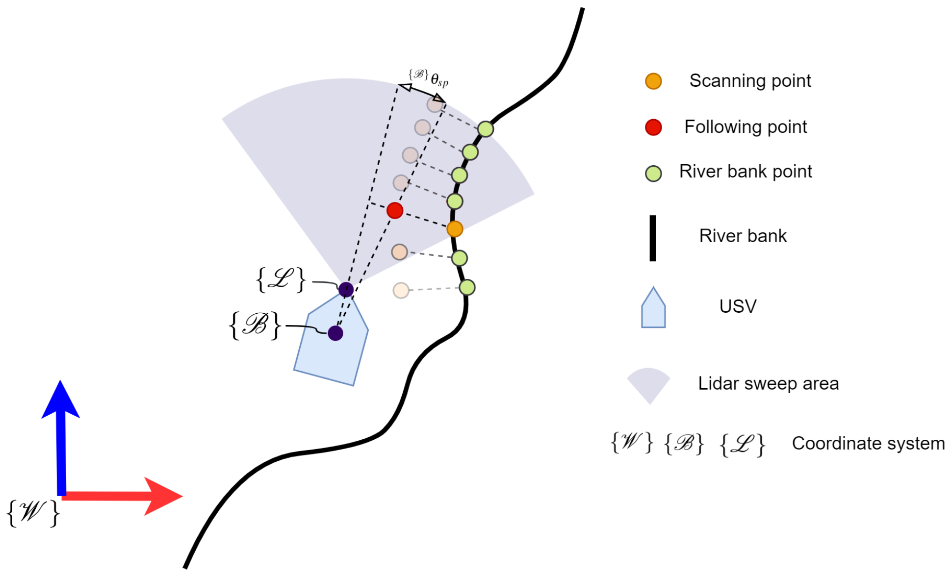
As shown in Figure 2, there are three coordinate frames to describe the motion of the USV system. $\left\{\mathcal{W}\right\}$ represents the fixed world frame, $\left\{\mathcal{L}\right\}$ represents the LiDAR frame and $\left\{\mathcal{B}\right\}$ represents the body frame on the center of the USV. The green riverbank points represent all LiDAR points reflected on the riverbank. The orange one is the scanning point which is selected as the bank shape reference point within the field-of-view (FOV). The red one is the USV following point, which is the waypoint for USV guidance.

A set of scanned PCD in the LiDAR frame $\left\{\mathcal{L}\right\}$ is denoted as:

$${}^{\left\{\mathcal{L}\right\}}p_i=\{(x_i,y_i)\in {\mathbb{R}}^2|i=1,\dots ,N_p\}$$

(1)

where ${}^{\left\{\mathcal{L}\right\}}p_i$ is the position of scanned points in the LiDAR frame. i is the index of each point in a single scan. $N_p$ is the number of scanned points. Then, we transform the ${}^{\left\{\mathcal{L}\right\}}p_i$ into the USV body frame $\left\{\mathcal{B}\right\}$, which is written as ${}^{\left\{\mathcal{B}\right\}}p_i$.

The scanning point is the LiDAR point that has the minimum Euclidean distance in the set ${}^{\left\{\mathcal{B}\right\}}p^{\ast }$, which is denoted as:

$${}^{\left\{\mathcal{B}\right\}}p^{\ast }=\{{}^{\left\{\mathcal{B}\right\}}p_j,\mathrm{where}j=\underset{i}{min}\parallel {}^{\left\{\mathcal{B}\right\}}p_i\parallel \}$$

(2)

Then we transform the ${}^{\left\{\mathcal{B}\right\}}p^{\ast }$ into the world frame $\left\{\mathcal{W}\right\}$ using ROS tf package [38], which is denoted as ${}^{\left\{\mathcal{W}\right\}}p^{\ast }$.

The following point ${}^{\left\{\mathcal{W}\right\}}\widehat{p}$ is calculated by:

$${}^{\left\{\mathcal{W}\right\}}\widehat{p}=\frac{\lambda }{\parallel {}^{\left\{\mathcal{W}\right\}}p\parallel }{}^{\left\{\mathcal{W}\right\}}p^{\ast }$$

(3)

where $\lambda$ is a pre-defined scaling parameter to determine the distance between the riverbank and the USV, the allowed range for $\lambda$ is [0, 1], a range established based on our experiments and simulation results to ensure the system’s stability and performance. Then we transform the following point into the USV body frame $\left\{\mathcal{B}\right\}$, denoted by ${}^{\left\{\mathcal{B}\right\}}\widehat{p}$.

3.3. RBFP Formulation

In order to navigate the USV to achieve the following point, the PID controller is implemented to complete the task. The yaw error setpoint ${\theta }_{sp}$ can be represented by the angle between the heading of USV and the following point, which is denoted as:

$${\theta }_{sp}=arccos\frac{{}^{\left\{\mathcal{B}\right\}}\mathbf{i}·{}^{\left\{\mathcal{B}\right\}}\widehat{p}}{\parallel {}^{\left\{\mathcal{B}\right\}}\mathbf{i}\parallel \parallel {}^{\left\{\mathcal{B}\right\}}\widehat{p}\parallel }$$

(4)

where ${}^{\left\{\mathcal{B}\right\}}\mathbf{i}$ is the basis vector of reference frame $\left\{\mathcal{B}\right\}$. It is aligned with the heading direction of the USV projected on the X–Y plane.

And the velocity setpoint $v_{sp}$ is defined as:

$$v_{sp}=\mu \parallel {}^{\left\{\mathcal{B}\right\}}\widehat{p}\parallel$$

(5)

where $\mu$ is a scaling factor based on the maximum velocity of the USV.

3.4. Controller Design

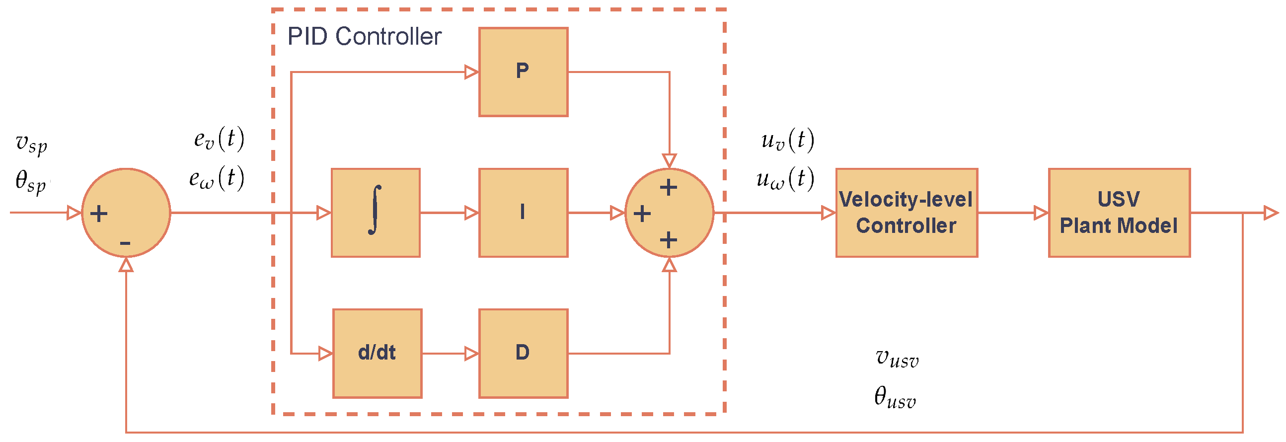
For the controller design of the USV, we have adopted the Proportional-Integral-Derivative (PID) for feedback control [39]. Following comprehensive testing in the Virtual RobotX high-fidelity simulation environment, our USV demonstrated strong performance in all these areas. Therefore, we can assert that the PID controller design we have adopted is highly effective for the motion control of USV. A PID controller in Figure 3 continuously calculates an error signal $e\left(t\right)$ by the difference between the reference signal $r\left(t\right)$ and a measurement $y\left(t\right)$ and then the sum of proportional, integral, and derivative terms as the feedback signal $u\left(t\right)$.

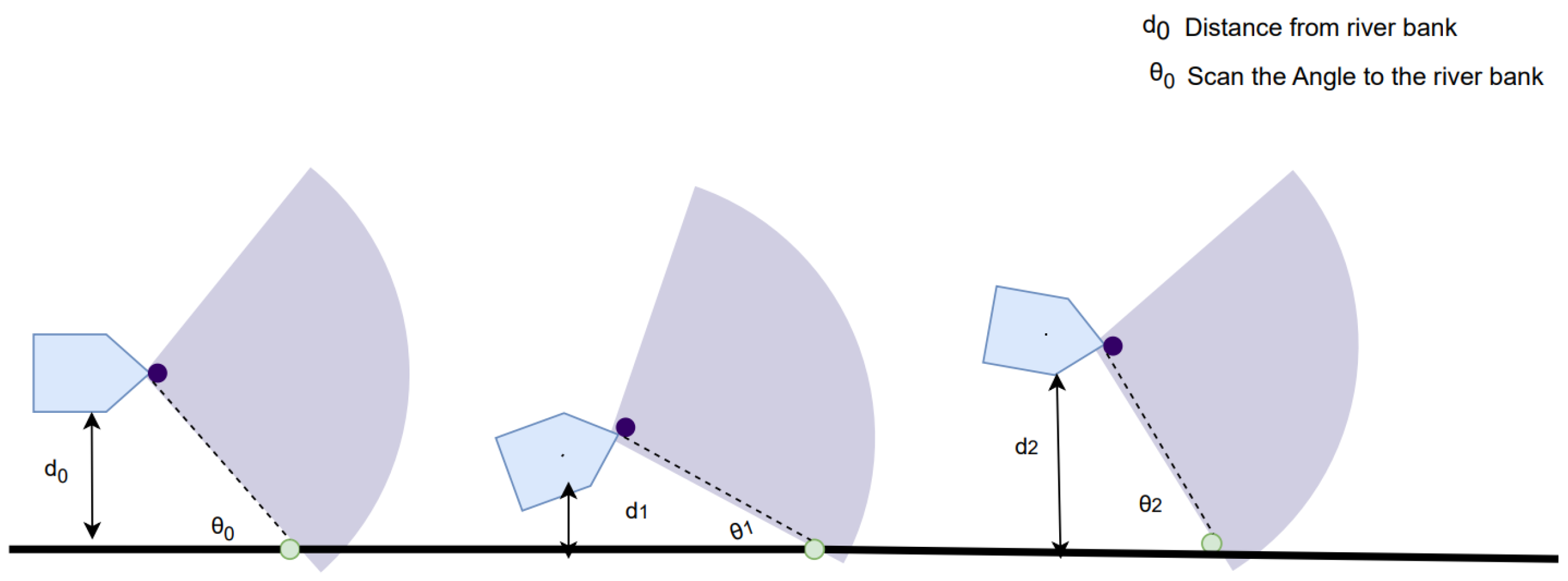
The USV distance from the riverbank is defined as $d_0$, and the angle between the first LiDAR line and the riverbank is set as ${\theta }_0$ during riverbank scans. As described in Figure 4, when the relative distance between USV and the riverbank is greater than or less than $d_0$, PID control helps the USV maintain the required linear velocity and angular velocity of the relative distance between the USV and the riverbank. After rapid adjustment, the path planning is continued according to the shape of the riverbank after the regression to the relative distance $d_0$.

For instance, the reference signal for each control loop is the $e_v$ and $e_{\omega }$. The measurement is the estimated speed and yaw angle of the USV using the onboard sensors. The feedback signal is the setpoint of the linear velocity and angular velocity.

In our implementation, the PID controller is implemented to track the yaw speed error setpoint ${\theta }_{sp}$ and the velocity setpoint $v_{sp}$. Since the controller is formulated on the body frame, we omit the prefix of the coordinate frame. Let $\theta \in \mathbb{R}$ and $v_{usv}\in {\mathbb{R}}^2$ in world frame $\left\{\mathcal{W}\right\}$ represent the velocity and heading of the USV. The error of yaw speed and velocity that need to be compensated is denoted as

$$e_v\left(t\right)=v_{sp}\left(t\right)-v_{usv}\left(t\right)$$

(6)

$$e_{\omega }\left(t\right)={\theta }_{sp}\left(t\right)-{\theta }_{usv}\left(t\right)$$

(7)

To compensate for the error, we implement PID controllers to track the error, which are denoted as

$$u_v\left(t\right)=K_{\mathrm{p}2}{e}_v+K_{\mathrm{i}2}{\int }_0^t{e}_v\left(\tau \right)\mathrm{d}\tau +K_{\mathrm{d}2}\frac{\mathrm{d}{e}_v}{\mathrm{d}t}$$

(8)

$$u_{\omega }\left(t\right)=K_{\mathrm{p}1}{e}_{\omega }+K_{\mathrm{i}1}{\int }_0^t{e}_{\omega }\left(\tau \right)\mathrm{d}\tau +K_{\mathrm{d}1}\frac{\mathrm{d}{e}_{\omega }}{\mathrm{d}t}$$

(9)

where $K_{p1}$, $K_{i1}$, $K_{d1}$, $K_{p2}$, $K_{i2}$, $K_{d2}$ are parameters of the PID controller.

For differential thrust with fixed two aft thrusters configuration, the simplified differential drive-based equations of motion of the USV are written as [40]

$$v_{usv}=\alpha \left(T_r+T_{\mathcal{l}}\right)$$

(10)

$${\omega }_{usv}=\beta \left(T_r-T_{\mathcal{l}}\right)$$

(11)

where $T_r$ and $T_{\mathcal{l}}$ represent the proportion thrust of the right engine and left engine, respectively. $\alpha$ and $\beta$ are scaling coefficients, depending on the size of the USV and the distance between the two engines.

However, the model (10) and (11) is not natural to understand how fast the USV is moving and turning. Then, we represent the motion of the USV using wheel velocities in terms of variables v and $\omega$ by algebraic operations in order to intuitively allocate motion control. The inverse kinematics of the USV is denoted as

$$T_r=\frac{\beta v_{usv}+\alpha {\omega }_{usv}}{2\alpha \beta }$$

(12)

$$T_{\mathcal{l}}=\frac{\beta v_{usv}-\alpha {\omega }_{usv}}{2\alpha \beta }$$

(13)

The motion control mixer maps the linear velocity and angular rate of the USV to proportion thrusts based on our USV configuration. The thrust command is proportional to the pulse-width modulation (PWM) setpoint. Therefore, the transformation of the PWM setpoints for the actuators is defined as

$${pwm}_r=\frac{\beta u_v+\alpha u_{\omega }}{2\alpha \beta }$$

(14)

$${pwm}_{\mathcal{l}}=\frac{\beta u_v-\alpha u_{\omega }}{2\alpha \beta }$$

(15)

To ensure the PWM value is valid and safe for the system within a feasible range, the PWM limiter is defined as

$$\begin{array}{c}\hfill pw{m}_{out,i}=\left\{\begin{array}{cc}pw{m}_{min}\hfill & ,pw{m}_i<pw{m}_{min}\hfill \\ pw{m}_i\hfill & ,pw{m}_{min}\le pw{m}_i\le pw{m}_{max}\hfill \\ pw{m}_{max}\hfill & ,pw{m}_i>pw{m}_{max}\hfill \end{array}\right.\end{array}$$

(16)

where $i=\{r,\mathcal{l}\}$ and $pw{m}_{max}$ and $pw{m}_{min}$ is the maximum and minimum PWM value setpoint, respectively.

To sum up, we formulate the riverbank following planner, which calculates the heading and velocity setpoints based on the 2D LiDAR scanner. Then, we derive the inverse kinematic of the USV with differential thrust with fixed two aft thrusters configuration, which maps the desired linear and angular velocity command to the desired motor PWM setpoints. A PID controller is iteratively implemented to compensate for the error of yaw and linear velocity. Thus, our planner does not need to manually set the target point to guide the USV on navigation, and can also adjust the distance to the riverbank according to the practical mission requirements. Moreover, RBFP has been implemented in the ROS simulation environment and can be easily migrated to the real world to accomplish specific tasks.

4. Experiments

4.1. High-Fidelity ROS Simulation

We use a Virtual RobotX (VRX) environment to simulate the riverbank to achieve high-precision experimental simulation. During the simulation, the USV will be equipped with a 2D LiDAR to scan the riverbank and plan a path similar to the riverbank by transmitting the scanned point cloud information to the controller. We added wind as an external influence to become closer to the real-world environment. Thus, we use kinematic control to develop a path planner in this study, which can simplify the control problem, reduce computational complexity, and ignore the nonlinear dynamic characteristics of the USV, which can help us focus on the motion state variables, such as position, velocity, and attitude. Meanwhile, in empirical trials, Holland [41] successfully linked VRX to an actual USV, substantiating that the path planning and data gathered in both simulated and real-world environments bear remarkable similarities.

4.1.1. Virtual RobotX

Virtual RobotX (VRX) [42], based on Gazebo simulation and Robotic Operating System (ROS) [43,44], provides high-fidelity simulation for USVs in complex marine environments. At the same time, VRX extends the Gazebo simulator to include wind and wave models, while increasing surface buoyancy to support a wide range of simulation scenarios. The following features of VRX strongly support our high-fidelity simulation:

• Random or fixed wind speed represents the effect on the motion of USVs.
• LiDAR simulation, including interaction with the riverbank.
• Six degree-of-freedom models for USVs with configurable actuators.

The detail of the high-fidelity simulation approach of VRX is described in Bingham’s work [42], including a wave model that applies Gerstner waves and the Pierson Moskowitz spectrum to simulate visual and physical effects, a wind model based on the Harris spectrum to represent both mean and variable components. Moreover, a parameterized propulsion model and a six-degrees-of-freedom vessel model accurately capture the influence of the environment and control on the motion of USVs and sensor perception.

Therefore, VRX is a perfect tool for high-precision simulation of the real-world water environment.

In Figure 5, we select three special riverbanks in the VRX environment to test the performance of RBFP, which are straight riverbank, convex riverbank, and concave riverbank. These three riverbank scenarios summarize all the riparian shapes USVs encounter in the real world.

4.1.2. Simulation Parameters and Implementation Details

We configured the USV with two articulated tail thrusters at the rear end of the USV and added a 2D LiDAR on the top of the USV to ensure that the scanned data were not biased. The average wind velocity is set to 0 m/s, 0.5 m/s, 1.0 m/s and 2.0 m/s, respectively.

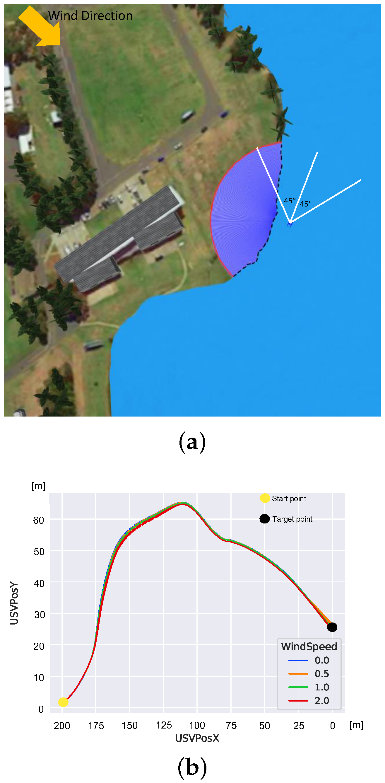
We obtain the states of the USV from Gazebo ground truth to reduce noise and uncertainty of state estimation. In reality, the range of LiDAR is 360 degrees. However, the installation position of LiDAR may sometimes be obstructed by the USV’s body, antenna, or payload. Considering the limited FOV of single-channel image transmission and the camera, we set a smaller FOV to overlap the camera and radar field-of-view, facilitating users in first-person teaching monitoring the ship’s operating status and reducing the blind area of the view. In the program, the USV LiDAR only tracks the riverbank shape 45 degrees to the left and right in front, not considering the riverbank shape behind the USV. This is based on the specific requirements and available equipment selection of our project. The three different scenarios we selected are the most representative points chosen from the entire map. Due to the three-dimensional shape of the map in Gazebo, it is impossible to precisely identify the edge of the map, hence the riverbank shape is not included in Figure 6b, Figure 7b and Figure 8b. We scan the riverbank with a laser radar on the USV to obtain the relative distance to the riverbank for the following.

Table 1. VRX simulation parameters setting.

Variable [Unit]	Value	Description
wave_gain [1]	0.1	Gain of wavefield model envelope
wave_period [s]	5.0	Peak period of wavefield model envelop
wave_angle [deg]	0.4	Horizontal angles of the constituent waves
wave_dx [m]	1.0	Wave direction in x-axis
wave_dy [m]	0.0	Wave direction in y-axis
LiDAR FOV [deg]	[−45, 45]	Field of view of 2D LiDAR sensor
wind_mean_vel [m/s]	0, 0.5, 1, 2	Constant mean wind speed
wind_direction [deg]	135	Constant wind direction
wind_std [m/s]	1.5	Standard deviation of the wind speed
distance_to_bank [m]	20	Distance between the USV and riverbank
$v_{max}$ [m/s]	1.0	Maximum linear velocity of the USV
${\omega }_{max}$ [rad/s]	1.0	Maximum angular velocity of the USV

summarizes the parameters of the simulation environment and algorithms. Additionally, the parameters for the USV dynamics in Gazebo use default values presented in VRX.

4.2. Simulation Results

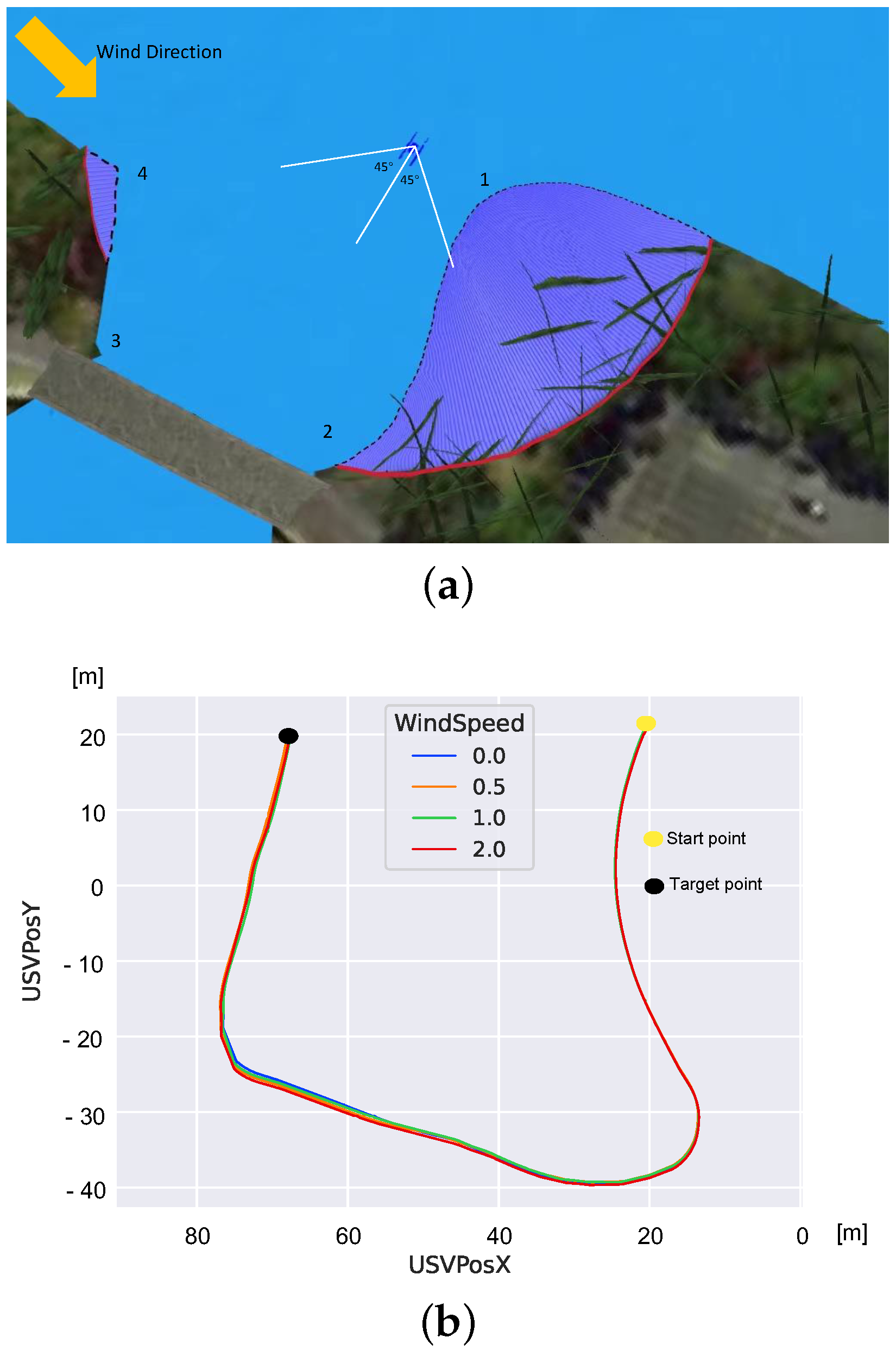
We verify the performance of the planner by using straight, convex, and concave banks, respectively, in the VRX. For the three bank shapes, the relative distance between the USV and the riverbank is set to 20 m, and the wind speed was set at 0, 0.5, 1.0, and 2.0 m/s, respectively. The relative distance between the USV and the riverbank is used to judge whether the RBFP can control the USV to follow the shape of the riverbank during autonomous navigation. In Figure 6b, Figure 7b and Figure 8b, curves in blue, orange, green, and red represent the USV planned path under different wind conditions. Five experiments were performed for each wind condition to obtain the confidence interval.

4.2.1. Results for Straight Riverbank

Figure 6a shows the test scenario of USV in the VRX environment. There is a relatively straight riverbank in the environment. The FOV of LiDAR is set from −45 to 45 degrees in VRX. The bright blue circle around the USV is the LiDAR scanning range. The black dotted line is the riverbank shape scanned by the LiDAR on the USV, and the red circle is the scanning range of the LiDAR. However, RBFP only intercepts the range within the white straight line region, that is, the FOV direction is from −45 to 45 degrees as the following direction. The yellow arrow indicates the direction of the wind. The planned path under different wind conditions is shown in Figure 6b with curves in different colors. In Figure 6b, the USV only needs to scan one side of the bank for following, so the planned path is very similar to the riverbank. During the test, the wind was blowing from the upper left corner to the lower right corner, which can drive the USV far away from the riverbank. Though the wind force will affect the planned path, the trajectory planned by the USV overlaps significantly. The reason for this is that the USV will measure the relative distance with the riverbank through the LiDAR, and control the navigation trajectory by adjusting the speed of the steering gear through PID when close to or far away from the riverbank, to ensure high precision following bank path planning. The path map is made by saving the waypoints traveled by the USV and adding error bands to show the possible location of the navigation under multiple experiments.

4.2.2. Results for Convex Riverbank

Convex banks exhibit similarities with straight banks; in both cases, the USV must follow one side of the bank for path planning. The distinct behavior emerges when the USV encounters the inflection point of the convex shape. Upon passing this point, the LiDAR scans the riverbank’s shape and promptly plans the path. The wind’s influence requires the PID controller to adjust the USV’s heading for accurate bank following. Figure 7a illustrates the USV’s behavior along a convex bank. In Figure 7b, the vertex of the convex bank is discernible at the position X = 90. Even after surpassing this vertex, the USV effectively scans the narrowing riverbank and persists in its path planning. Concurrently, a depression is observed at X = 120, which the USV detects and plans accordingly. Although wind factors might deviate the USV from its course, real-time adjustments via the PID controller ensure the USV rejoins its intended path when near the riverbank.

4.2.3. Results for Concave Riverbank

Concave banks present intricate challenges on the bank, as follows. During the USV’s scanning process, it frequently detects the opposite bank, which can hamper its ability to accurately trace the intended bank. The riverbank following planner mitigates this by utilizing a wide-angle LiDAR scan, ensuring a comprehensive capture of the surroundings. This allows for the precise identification of the riverbank’s shape and discernment of whether the opposite side is navigable, circumventing scenarios where one bank side is untraceable. In Figure 8a, positions 1 and 4 denote the USV’s entry and exit points of the concave bank, respectively. As the USV transitions between positions 2 and 3, its inherent momentum brings it closer to the riverbank. Concurrently, the PID controller intervenes to rectify the USV’s heading, minimizing path deviations. Should the USV, while within the concave bank, detect the opposite bank, the planner strategically disregards it and prioritizes the USV’s proximal bank for navigation. Figure 8b showcases the USV’s planned trajectory within the concave bank under varied wind influences. Due to both its dynamics and wind impact, the USV tends to veer toward the riverbank, especially during turns.

4.3. Statistics

The boxplot in Figure 9 shows a five-digit visual representation of the distance between the USV and the riverbank under four wind conditions and three different riverbank shapes of straight, convex, and concave banks. The five-number summary is the mean (and 50% quartile), 25% quartile, 75% quartile, maximum, and minimum. The median of relative distance in the three scenarios is closely distributed at 21 m. The box plot is comparatively short, suggesting that overall relative distances have a stable performance with each other. In the straight case, the interquartile range (IQR) is the smallest compared with the other two cases. This renders that the proposed method has achieved the best performance doing straight bank following. The IQR in the straight case has a minimum IQR of about 0.5 m. The IQR for convex and concave cases are about 3 and 4 m, respectively. It means that the USV encounters a convex or concave shape on the path, when the error in the desired heading suddenly becomes larger, while the USV maintains the linear speed of the previous timestamp due to inertia. Therefore, the riverbank distance is suddenly larger when compensating for the heading error. In engineering practice, the PID controllers we use are based on the compensation of errors to achieve control. Their delay leads to large errors but within acceptable limits.

Table 2. The relative distance of the USV from the riverbank.

Scenario	Wind	Max [m]	Min [m]	Mean [m]	Variance [m]	±15% Error Ratio
Straight	0.0	23.67	19.58	20.99	0.43	96.97%
	0.5	23.68	19.57	20.98	0.42	96.99%
	1.0	23.76	19.58	20.99	0.43	96.89%
	2.0	23.85	19.59	21.02	0.44	96.82%
Convex	0.0	35.68	8.34	21.42	24.95	66.97%
	0.5	35.69	8.25	21.36	24.65	67.27%
	1.0	35.69	8.14	21.31	24.58	67.45%
	2.0	35.69	7.86	21.23	25.12	67.51%
Concave	0.0	35.69	4.48	20.94	14.31	61.23%
	0.5	35.59	4.49	20.92	14.51	61.23%
	1.0	35.63	4.47	20.95	14.76	60.90%
	2.0	35.61	4.50	20.90	14.83	61.23%

shows the observations in all the tests. We take ±15% of the relative distance between the USV and the riverbank as the interval for high precision following the riverbank, which is called the following performance. We established a margin of 15%, which is grounded on extensive testing and evaluation, ensuring the reliability and robustness of our following algorithm. The following performance is assessed based on the ability to maintain a 20 m distance from the riverbank, allowing a ±15% error margin. This criterion was not arbitrarily chosen but is a result of comprehensive analysis and experimentation, reinforcing the credibility and feasibility of our method in real-world applications. We can see that the USV achieved 96.92% following the performance average of those 4 values in different wind speeds in the straight riverbank, perfectly achieving the desired results. At the same time, its mean is minimal, which proves that the oscillation amplitude of USV is small and the path is smooth. In convex banks, the shape of the bank drops rapidly after the raised vertex, so it takes time for the USV to complete the scanning and following of the bank. At the same time, when the relative distance between the USV and the riverbank increases, the USV will gradually approach the direction of the riverbank through PID control, increasing the mean value and variance of the relative distance between the USV and the riverbank, the results show that the following performance can reach 67.30%. In the concave bank, the minimum value of the USV and riverbank is smaller than that in the convex bank. This is because in the concave scenario, the dynamic of the USV causes it to deviate from the planned path when approaching the riverbank, and the PID controller helps the USV return to the original path. However, the decreased variance demonstrates that the USV has a high level of precision in following the planned path in this scenario. The result shows that the following performance can reach 60.90%. Because the RBFP takes into account that the wind affects the path planning and corrects the path in time when deviations occur, we obtain similar results with very few deviations when we set different wind speeds in the simulation.

5. Conclusions and Future Work

This paper introduced an innovative riverbank following planner (RBFP) for USVs. This planner leverages a 2D LiDAR to scan riverbank shapes, enabling the USV to autonomously generate navigation paths without the need for manually predefined waypoints. Within the VRX simulation environment, where wind force was introduced as an external perturbation, our planner demonstrated remarkable proficiency. For straight banks, 96.92% of the path exhibited deviations confined within 15% of the relative distance. Even in more intricate convex and concave banks, 67.30% and 61.15% path following efficiency was achieved.

The RBFP notably addresses a significant challenge in traditional path planning: the laborious task of setting accurate target points, especially when the riverbank’s morphology is elusive. Such adaptability is indispensable for tasks like riverbank safety inspections and underwater pipe detection. However, one limitation of the proposed planner is evident. Strong winds and turbulent waves can influence the USV’s orientation, making the LiDAR scans prone to fluctuations. While filters like the Kalman filter might refine the raw point cloud data, they could introduce latency, potentially jeopardizing the algorithm’s real-time efficacy.

In the future, it is imperative to field-test the RBFP on an actual USV, validating its capabilities outside of controlled simulations. Given the potential external disruptions in real-world settings, relying solely on IMUs might compromise pose accuracy. Consequently, our future endeavors will entail the fusion of RTK GPS with inertial sensors for enhanced state estimation. Furthermore, we aspire to harness multi-sensor fusion strategies—incorporating near-infrared cameras, millimeter-wave radar, and further LiDAR modalities—to counter external environmental interferences. By assimilating these avant-garde sensing techniques, we aim to fortify the precision and resilience of our riverbank following planner, ensuring its readiness for practical implementations.

References

1. Manley, J.E. Unmanned surface vehicles, 15 years of development. In Proceedings of the OCEANS, Quebec City, QC, Canada, 15–18 September 2008; pp. 1–4. [Google Scholar]
2. Jorge, V.A.; Granada, R.; Maidana, R.G.; Jurak, D.A.; Heck, G.; Negreiros, A.P.; Dos Santos, D.H.; Gonçalves, L.M.; Amory, A.M. A survey on unmanned surface vehicles for disaster robotics: Main challenges and directions. Sensors 2019, 19, 702. [Google Scholar] [CrossRef] [PubMed]
3. Specht, M.; Specht, C.; Szafran, M.; Makar, A.; Dąbrowski, P.; Lasota, H.; Cywiński, P. The use of USV to develop navigational and bathymetric charts of yacht ports on the example of national sailing centre in Gdańsk. Remote Sens. 2020, 12, 2585. [Google Scholar] [CrossRef]
4. Veers, J.; Bertram, V. Development of the USV multi-mission surface vehicle III. In Proceedings of the 5th International Conference on Computer Applications and Information Technology in the Maritime Industries, Drübeck, Germany, 23–25 May 2006. [Google Scholar]
5. Chen, H.; Zhu, C.; Chen, J.; Peng, Y.; Yao, J. Design of Unmanned Surface Vehicle for Submarine Pipeline Detection. In Proceedings of the 2018 IEEE 4th Information Technology and Mechatronics Engineering Conference (ITOEC), London, UK, 14–16 December 2018; pp. 198–202. [Google Scholar] [CrossRef]
6. Kurowski, M.; Thal, J.; Damerius, R.; Korte, H.; Jeinsch, T. Automated survey in very shallow water using an unmanned surface vehicle. IFAC-PapersOnLine 2019, 52, 146–151. [Google Scholar] [CrossRef]
7. Zhu, M.; Wang, Y.; Wen, Y. A Global Path Planning Algorithm of Unmanned Vessel in Inland Waterway. In ICTIS 2013: Improving Multimodal Transportation Systems-Information, Safety, and Integration; ASCE: Reston, VA, USA, 2013; pp. 2106–2113. [Google Scholar]
8. Yang, P.; Song, C.; Chen, L.; Cui, W. Image Based River Navigation System of Catamaran USV with Image Semantic Segmentation. In Proceedings of the 2022 WRC Symposium on Advanced Robotics and Automation (WRC SARA), Beijing, China, 20 August 2022; pp. 147–151. [Google Scholar] [CrossRef]
9. Scherer, S.; Rehder, J.; Achar, S.; Cover, H.; Chambers, A.; Nuske, S.; Singh, S. River mapping from a flying robot: State estimation, river detection, and obstacle mapping. Auton. Robot. 2012, 33, 189–214. [Google Scholar] [CrossRef]
10. Son, N.S.; Yoon, H.K. Study on a waypoint tracking algorithm for unmanned surface vehicle (USV). J. Navig. Port Res. 2009, 33, 35–41. [Google Scholar] [CrossRef]
11. Stateczny, A.; Wlodarczyk-Sielicka, M.; Gronska, D.; Motyl, W. Multibeam Echosounder and LiDAR in process of 360-degree numerical map production for restricted waters with HydroDron. In Proceedings of the 2018 Baltic Geodetic Congress (BGC Geomatics), Olsztyn, Poland, 21–23 June 2018; pp. 288–292. [Google Scholar]
12. Zhuang, Y.; Sun, Y.; Wang, W. Mobile robot hybrid path planning in an obstacle-cluttered environment based on steering control and improved distance propagating. Int. J. Innov. Comput. Inf. Control 2012, 8, 4095–4109. [Google Scholar]
13. Zhou, C.; Gu, S.; Wen, Y.; Du, Z.; Xiao, C.; Huang, L.; Zhu, M. The review unmanned surface vehicle path planning: Based on multi-modality constraint. Ocean Eng. 2020, 200, 107043. [Google Scholar] [CrossRef]
14. Wang, Z.; Liang, Y.; Gong, C.; Zhou, Y.; Zeng, C.; Zhu, S. Improved dynamic window approach for Unmanned Surface Vehicles’ local path planning considering the impact of environmental factors. Sensors 2022, 22, 5181. [Google Scholar] [CrossRef]
15. Khatib, O. Real-time obstacle avoidance for manipulators and mobile robots. In Autonomous Robot Vehicles; Springer: Berlin/Heidelberg, Germany, 1986; pp. 396–404. [Google Scholar]
16. Chu, Y.; Wu, Z.; Yue, Y.; Zhu, X.; Lim, E.G.; Paoletti, P. PK-APF: Path-Keeping Algorithm for USVs Based on Artificial Potential Field. Appl. Sci. 2022, 12, 8201. [Google Scholar] [CrossRef]
17. Zhang, L.; Mou, J.; Chen, P.; Li, M. Path planning for autonomous ships: A hybrid approach based on improved apf and modified vo methods. J. Mar. Sci. Eng. 2021, 9, 761. [Google Scholar] [CrossRef]
18. Lin, P.; Choi, W.Y.; Chung, C.C. Local path planning using artificial potential field for waypoint tracking with collision avoidance. In Proceedings of the 2020 IEEE 23rd International Conference on Intelligent Transportation Systems (ITSC), Rhodes, Greece, 20–23 September 2020; pp. 1–7. [Google Scholar]
19. Ngah, W.; Buniyamin, N.; Mohamad, Z. Point to point sensor based path planning algorithm for autonomous mobile robots. In Proceedings of the 9th WSEAS International Conference on System Science and Simulation in Engineering, Tenerife, Spain, 16–18 December 2010; pp. 186–191. [Google Scholar]
20. Lumelsky, V.; Stepanov, A. Dynamic path planning for a mobile automaton with limited information on the environment. IEEE Trans. Autom. Control 1986, 31, 1058–1063. [Google Scholar] [CrossRef]
21. Ng, J.; Bräunl, T. Performance comparison of bug navigation algorithms. J. Intell. Robot. Syst. 2007, 50, 73–84. [Google Scholar] [CrossRef]
22. Yufka, A.; Parlaktuna, O. Performance comparison of bug algorithms for mobile robots. In Proceedings of the 5th International Advanced Technologies Symposium, Karabuk, Turkey, 4–7 September 2009; pp. 13–15. [Google Scholar]
23. Feng, P.; Wu, J.; Yang, X.; Zhang, W.; Guo, H. Design and Realization of LQR Course Keeping Control for Small Unmanned Surface Vehicle. In Proceedings of the 2021 China Automation Congress (CAC), Beijing, China, 22–24 October 2021; pp. 6640–6645. [Google Scholar] [CrossRef]
24. Peng, Y.; Li, Y. Autonomous Trajectory Tracking Integrated Control of Unmanned Surface Vessel. J. Mar. Sci. Eng. 2023, 11, 568. [Google Scholar] [CrossRef]
25. Bingul, Z.; Gul, K. Intelligent-PID with PD Feedforward Trajectory Tracking Control of an Autonomous Underwater Vehicle. Machines 2023, 11, 300. [Google Scholar] [CrossRef]
26. Fan, Y.; Sun, X.; Wabg, G.; Guo, C. On fuzzy self-adaptive PID control for USV course. In Proceedings of the 2015 34th Chinese Control Conference (CCC), Hangzhou, China, 28–30 July 2015; pp. 8472–8478. [Google Scholar]
27. Fefilatyev, S.; Goldgof, D.; Shreve, M.; Lembke, C. Detection and tracking of ships in open sea with rapidly moving buoy-mounted camera system. Ocean Eng. 2012, 54, 1–12. [Google Scholar] [CrossRef]
28. Mou, X.; Wang, H. Image-based maritime obstacle detection using global sparsity potentials. J. Inf. Commun. Converg. Eng. 2016, 14, 129–135. [Google Scholar] [CrossRef]
29. Prasad, D.K.; Rajan, D.; Prasath, C.K.; Rachmawati, L.; Rajabally, E.; Quek, C. MSCM-LiFe: Multi-scale cross modal linear feature for horizon detection in maritime images. In Proceedings of the 2016 IEEE Region 10 Conference (TENCON), Singapore, 22–25 November 2016; pp. 1366–1370. [Google Scholar]
30. Liu, H.; Javed, O.; Taylor, G.; Cao, X.; Haering, N. Omni-directional surveillance for unmanned water vehicles. In Proceedings of the Eighth International Workshop on Visual Surveillance-VS2008, Santorini, Greece, 6–8 June 2008. [Google Scholar]
31. Kristan, M.; Kenk, V.S.; Kovačič, S.; Perš, J. Fast image-based obstacle detection from unmanned surface vehicles. IEEE Trans. Cybern. 2015, 46, 641–654. [Google Scholar] [CrossRef]
32. Alpert, S.; Galun, M.; Brandt, A.; Basri, R. Image segmentation by probabilistic bottom-up aggregation and cue integration. IEEE Trans. Pattern Anal. Mach. Intell. 2011, 34, 315–327. [Google Scholar] [CrossRef]
33. Xu, S.; Ye, N.; Xu, S. A new method for shoreline extraction from airborne LiDAR point clouds. Remote Sens. Lett. 2019, 10, 496–505. [Google Scholar] [CrossRef]
34. Lee, I.C.; Cheng, L.; Li, R. Optimal parameter determination for mean-shift segmentation-based shoreline extraction using lidar data, aerial orthophotos, and satellite imagery. In Proceedings of the ASPRS Conference, Orlando, FL, USA, 15–18 November 2010. [Google Scholar]
35. Liu, H.; Wang, L.; Sherman, D.J.; Wu, Q.; Su, H. Algorithmic foundation and software tools for extracting shoreline features from remote sensing imagery and LiDAR data. J. Geogr. Inf. Syst. 2011, 3, 99. [Google Scholar] [CrossRef]
36. Lee, I.C.; Wu, B.; Li, R. Shoreline extraction from the integration of lidar point cloud data and aerial orthophotos using mean-shift segmentation. In Proceedings of the ASPRS Annual Conference, Baltimore, MA, USA, 3–6 June 2009; Volume 2, pp. 3033–3040. [Google Scholar]
37. Li, W.; Liu, H.; Qin, C. A method for the extraction of shorelines from airborne lidar data in muddy areas and areas with shoals. Remote Sens. Lett. 2022, 13, 480–491. [Google Scholar] [CrossRef]
38. tf—ROS Wiki. Available online: http://wiki.ros.org/tf (accessed on 23 July 2023).
39. Stateczny, A.; Burdziakowski, P. Universal autonomous control and management system for multipurpose unmanned surface vessel. Pol. Marit. Res. 2019, 26, 30–39. [Google Scholar] [CrossRef]
40. Klinger, W.B.; Bertaska, I.R.; von Ellenrieder, K.D.; Dhanak, M.R. Control of an Unmanned Surface Vehicle with Uncertain Displacement and Drag. IEEE J. Ocean. Eng. 2017, 42, 458–476. [Google Scholar] [CrossRef]
41. Holland, D.; Landaeta, E.; Montagnoli, C.; Ayars, T.; Barnes, J.; Barthelemy, K.; Brown, R.; Delp, G.; Garnier, T.; Halleran, J.; et al. Design of the Minion Research Platform for the 2022 Maritime RobotX Challenge. Available online: https://robotx.org/programs/robotx-challenge-2022/ (accessed on 10 October 2023).
42. Bingham, B.; Aguero, C.; McCarrin, M.; Klamo, J.; Malia, J.; Allen, K.; Lum, T.; Rawson, M.; Waqar, R. Toward Maritime Robotic Simulation in Gazebo. In Proceedings of the MTS/IEEE OCEANS Conference, Seattle, WA, USA, 4–7 October 2019. [Google Scholar]
43. Quigley, M.; Conley, K.; Gerkey, B.; Faust, J.; Foote, T.; Leibs, J.; Wheeler, R.; Ng, A.Y. ROS: An open-source Robot Operating System. In Proceedings of the ICRA Workshop on Open Source Software, Kobe, Japan, 8–12 July 2009; Volume 3, p. 5. [Google Scholar]
44. Quigley, M.; Gerkey, B.; Smart, W.D. Programming Robots with ROS: A Practical Introduction to the Robot Operating System; O’Reilly Media, Inc.: Sebastopol, CA, USA, 2015. [Google Scholar]
Figure 1. System framework.
Applsci 13 11319 g001
Figure 2. USV follows by scanning the riverbank.
Applsci 13 11319 g002
Figure 3. PID Controller.
Applsci 13 11319 g003
Figure 4. PID controller solves the USV path deviation.
Applsci 13 11319 g004
Figure 5. River banks in VRX environment. 1, 2 and 3 represent straight, convex and concave banks, respectively.
Applsci 13 11319 g005
Figure 6. USV follows a straight riverbank (a) VRX test environment; (b) The USV planned path on a straight riverbank.
Applsci 13 11319 g006
Figure 7. USV follows a convex riverbank (a) VRX test environment; (b) The USV planned path on a convex riverbank.
Applsci 13 11319 g007
Figure 8. USV follows a concave riverbank (a) VRX test environment; (b) The USV planned path on a concave riverbank.
Applsci 13 11319 g008
Figure 9. Boxplot of Relative Distance. (a) Straight Riverbank. (b) Convex Riverbank. (c) Concave Riverbank.
Applsci 13 11319 g009