Study of the Relationships among the Reverse Torque, Vibration, and Input Parameters of Mud Pumps in Riserless Mud Recovery Drilling

Abstract

Compared with traditional deepwater drilling, riserless mud recovery (RMR) drilling technology has the advantages of improving drilling efficiency, reducing risks, and minimizing environmental effects. Therefore, RMR drilling technology has been widely applied in recent years. This study primarily investigates the relationships among reverse torque, vibration, and input parameters of mud pumps in riserless mud recovery drilling. Firstly, the operating principle and the structure of the mud pump module are analyzed, and an analytical model for the reverse torque and the vibration of the mud pump is established. Secondly, relevant data are derived from theoretical calculations and experiments, and the relationships among the reverse torque, vibration, and input parameters of the mud pump are analyzed using ANSYS (Version 2020 R1) software. Furthermore, the SVR (support vector regression) algorithm is employed to predict and analyze the amplitude of the mud pump’s vibration. Finally, the conclusions are drawn based on the findings of the relationships among the reverse torque, vibration, and input parameters of the mud pump. The findings show that the reverse torque of the mud pump increases approximately linearly with an increase in rotational speed, and the vibration of the mud pump increases and then decreases with an increase in rotational speed. The predicted values obtained through the prediction algorithm closely match the actual values. The findings provide a valuable reference for the application of RMR technology.

1. Introduction

Although marine oil and gas resources are abundant, deepwater drilling is facing many technical challenges. RMR technology can improve the efficiency of drilling processes, reduce environmental effects, and increase operational flexibility [1,2,3]. Dual-gradient drilling technology is an unconventional drilling technology, which changes the annular pressure gradient of the riser through the pump or changes the fluid density. This technology can address some issues related to formation pressure in deepwater drilling [4,5,6,7,8]. Riserless mud recovery drilling (RMR) [9] is an implementation solution for dual-gradient drilling. It forms a closed mud circulation system, allowing mud to be recovered and significantly reducing the amount of mud used. Additionally, it avoids discharging mud into the seawater, thereby protecting the marine environment. RMR is widely used in deep-sea offshore drilling.

Li et al. [10] analyzed the effects of seawater depth, equivalent static density (ESD) of drilling fluid, drilling chip concentration, and discharge on the annular pressure and ECD of an RMR system based on drilling data from a vertical well in the South China Sea. Reynolds et al. [11] presented a pioneering case study for the Luiperd Mine and one of the measures for reducing environmental risk was to adopt a new articulation tool to minimize the bending stress applied to the subsea wellhead running tool (WHRT) and landing rope in running through the inflow pipe and surface casing. Claudey et al. [12] employed a controlled mud level technique in the Barents Sea, which controlled the liquid position within the riser, optimized the downhole pressure, prevented mud leakage, and maintained pressure balance. Claudey et al. [13] successfully deployed a riserless mud recovery (RMR) system at a water depth of 854 m, the deepest operation of its kind in the North Sea to date. Mud-lifting circulation was achieved without wellbore stability or shallow hazard issues, and no mud contamination occurred. Rosenberg et al. [14] introduced a design method for oil wells and used casing drilling to eliminate the need for multiple deep-water riserless series connections, enabling the high-pressure wellhead casing and its conductors to be set deeper. In the land and shallow sea environment, the practice of casing drilling has become very mature to improve drilling efficiency and reduce drilling hazards. RMR technology was also applied to achieve the successful cementing of the surface casing in the Malikai deepwater field in Sabah, Malaysia [15]. A model was devised to measure the bottomhole pressure of the RMR system during gas intrusion conditions using the gas–liquid two-phase flow theory [16]. In the Gulf of Mexico, RMR was initially implemented, leading to an enhanced improved operational efficiency and better wellbore structure [17]. The successful commercial application of dual-gradient drilling was first achieved in the ultra-deepwater Gulf of Mexico [18]. In the UK Continental Shelf (UKCS) oil-field development project, a RMR top-hole operation was employed for the first time [19]. Riserless dual-gradient technology was used for drilling highly deviated wells in the Santos Basin offshore Brazil, addressing issues related to formation erosion and wellbore collapse [20]. RMR has been utilized offshore multiple times, successfully resolving problems of loose sandstone soil and deepening surface casing, completing over 40 wells with a water depth of 450 m [21,22,23]. When drilling in overpressured zones [24,25,26,27], RMR can also compensate for the absence of a riser and blowout preventer (BOP). It has been utilized successfully in various offshore areas with loose formations and losses.

Mud pumps for drilling have also been studied by some researchers, in addition to RMR technology. In order to develop a system to monitor their technical conditions, Bejger et al. [28] investigated these pumps under operational conditions. Deng et al. [29] presented a practical diagnosis method that could effectively improve the fault diagnosis level for the fluid end of high-pressure reciprocating mud pumps. Khademi-Zahediet al. [30] utilized analytical studies and finite element methods to examine how different loading conditions impact the behaviors of mud pumps. Piasecki et al. [31] investigated mud pumps to develop an effective diagnostic tool that could help pump operators with their daily maintenance routines. ANSYS is a large-scale general-purpose finite element analysis software that can simulate and optimize a wide range of complex engineering problems. In this paper, pumps are analyzed using the ANSYS software. Additionally, the ANSYS software has numerous applications in other fields. ANSYS software was used by Bhatti et al. [32] to numerically model and evaluate the performance of a standing-wave thermoacoustic refrigerator with multiple stacks. The ANSYS Fluent software package was used by Hamdamov et al. [33] to conduct mathematical modeling of vertical axis wind turbines. ANSYS Fluent software was used by Ezzat et al. [34] to numerically simulate the phase transition process. Sohn et al. [35] used ANSYS and ANSYS pre-processor/post-processor composite material to create the layered composite material structure described in the article. Tjitra et al. [36] used ANSYS software to perform numerical simulation analysis of three-dimensional reinforced concrete beams under various collapse mechanisms.

However, few scholars have conducted analytical studies on the stability of mud pumps and their manifold connection employed in RMR technology, which is the core condition for the stable operation of RMR in the deep sea. During the drilling process, the deepwater RMR pump is mounted using a mid-hanging configuration, which results in reverse torque and vibration during normal operation. Hence, it is crucial to conduct a pertinent examination and investigation of the mud pump’s reverse torque and vibration in the mud return circulation system. This study examines the relationships among reverse torque, vibration, and input parameters of the mud pump within the mud return circulation system. The study’s contributions can be summarized as follows:

(I)

An analysis is conducted of the working principle and the structure of the mud pump module, and an analytical model for the reverse torque and vibration of the mud pump is developed.

(II)

Theoretical calculations and experiments are used to generate relevant data. The relationships among the reverse torque, vibration, and input parameters of the mud pump are analyzed using the ANSYS (Version 2020 R1) software.

(III)

Predicting and analyzing the amplitude of the mud pump vibration is achieved by employing the SVR algorithm.

(IV)

Relevant conclusions are drawn from the research results on the relationships among the reverse torque, vibration, and input parameters of the mud pump.

The findings show that the reverse torque of the mud pump increases approximately linearly with an increase in the rotational speed, and the vibration of the mud pump increases and then decreases with the increase in the rotational speed. The predicted values obtained through the prediction algorithm closely match the actual values.

2. Analysis of the Reverse Torque and Vibration in the Mud Pump

Due to the mid-hanging configuration of the deepwater RMR pump, it generates reverse torque and vibration in the mud return pipeline connected at both the upper end and the lower end during startup and operation. The return pipeline for the mud may be damaged, which will affect the stability and safety of both the mud pump and the return pipeline. In this section, the reverse torque and the vibration of the mud pump were analyzed using the ANSYS (Version 2020 R1) software. Since the mud pump used in the RMR technique is a ten-stage mud pump, a single-stage pump was first used for the analysis, and the error between the theoretical calculations and the simulation analysis was compared to ensure the error was within a reasonable range, thus proving the correctness of the analysis. Then, the mud pump (ten-stage pump) was analyzed based on the setup adopted for analyzing the single-stage pump.

Figure 1 shows the flowchart of the main analysis process. Firstly, the reverse torque of the single-stage mud pump was theoretically calculated and compared with the numerical simulation results as well as the error analysis. Secondly, the fluid model was established; its mesh division, materials, and boundary conditions were set; and the mud pump’s reverse torque and rotational speed were derived from the changes in the relationships. Finally, the rotor model of mud pump was established; its mesh division, materials, and boundary conditions were set; and the relationships between the mud pump’s vibration and the motor’s input parameters were obtained.

2.1. Working Principle and Structure of the Mud Pump Module

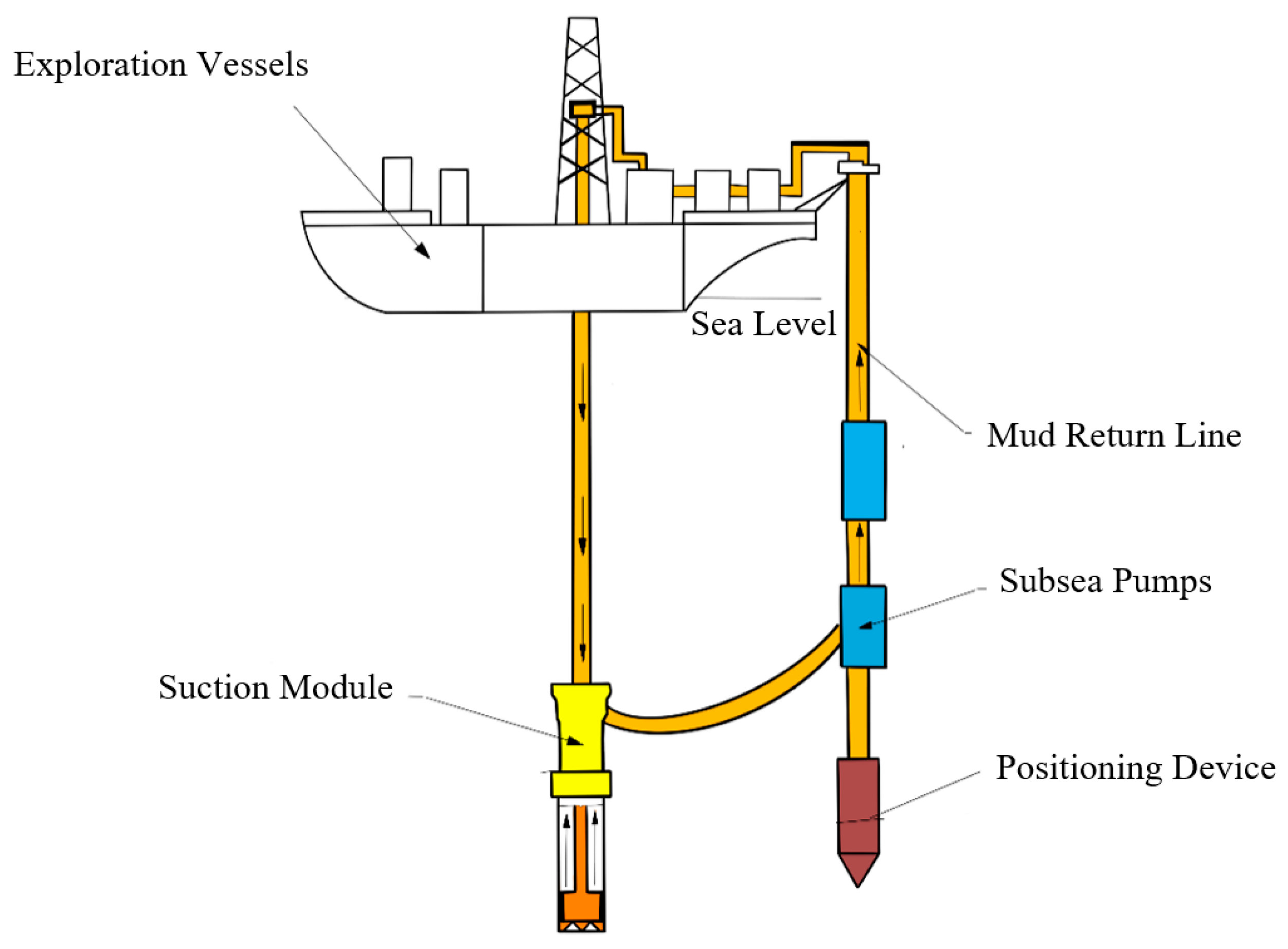
The riserless mud recovery (RMR) closed-loop drilling system generally consists of a drilling unit, a mud return system unit, a mud treatment unit, and a power monitoring unit. The operational mode of the RMR closed-loop system is shown in Figure 2. The mud pump module is located within the mud return system unit and is installed using a mid-hanging configuration on the mud-lifting pipeline. The main function of the mud pump module is to transport the cuttings generated by the suction module through the mud return pipeline to the surface mud treatment equipment. With the suction action of the subsea mud pump, drilling fluid is drawn from the lower outlet of the suction module, enters the subsea mud pump through the subsea drilling fluid delivery pipeline, and is then lifted to the drilling vessel for processing and subsequent reuse.

The mud pump module is used to circulate a mixture of drilling fluid, cuttings, and even gas. The external view of the mud pump module is shown in Figure 3. The mud pump is powered by the platform and all equipment is only subjected to the hydrostatic pressure of seawater. The mud pump module is a critical component of the riserless mud recovery closed-loop system. It controls the pressure balance inside the suction module using the subsea pump and facilitates the return of drilling mud. The subsea pump module is fixed on the mud return pipeline and not only needs to ensure the reliability of the entire pipeline structure but also to maintain the smooth flow of the mud return pipeline. To prevent a collision between the lower subsea pump module and the suction module during operation, a subsea anchor is used to secure the lower end of the mud return pipeline, and a tension force is applied to restrict the horizontal movement of the mud return pipeline.

The lifting module of the mud pump unit mainly consists of drill pipe joints, corrective blocks, ball valves, centrifugal pumps, a four-way connector, a skid assembly, a ball valve control device, a skid, a trolley adapter, a supporting mechanism, and other components. The skid is the foundation of the mud pump module and serves mainly for connection and support. During drilling operation, the skid is installed on the mud lifting pipeline using a center-hanging arrangement, providing support for the internal components of the mud pump module. The skid remains stationary during the mud-lifting process and does not undergo significant vibration. The centrifugal pump used in the module is a multistage centrifugal pump, which increases the power of the pump module, enabling it to meet the requirements of deepwater operation. The mud return riser provides a conduit for drilling mud to flow from the seabed wellhead to the drilling rig. It also serves to fix and support two lifting pump module units, bearing the weight of the seabed anchor and resisting the force applied by sea currents and the movement of the drilling rig.

2.2. Validation of the Theoretical Calculations and the Numerical Simulation Results for the Reverse Torque of the Single-Stage Mud Pump

2.2.1. Theoretical Calculations of the Reverse Torque for a Single-Stage Mud Pump

According to the principle of energy conservation, the torque work conducted by the single-stage mud pump on the mud can be divided into two parts: one portion is converted into an increase in the energy of the mud and another portion is lost due to friction in the pipeline. The portion that contributes to the increase in mud energy is considered useful, while the portion lost due to friction in the pipeline is considered useless. The energy of the mud includes pressure energy, potential energy, and kinetic energy. Since the single-stage mud pump selected has the same inlet and outlet pipe diameters, the kinetic energy of the mud at the inlet and outlet remains constant. The calculation formula for the increase in the pressure energy of the mud within a time unit is shown as follows [38], where ΔE_P is the pressure energy from the increase in mud within a time unit, ΔP is the pressure difference between the inlet and outlet, and Q is the mud volume flow.

$$\Delta E_P=\Delta PQ$$

(1)

The formula for calculating the increase in potential energy of mud per unit time is shown as follows [38], where ΔE_h is the potential energy from the increase in mud within a time unit, ∆h is the height difference between the inlet and outlet, ρ is the density of the mud, and g is the gravitational acceleration.

$$\Delta E_h=Q\rho g\Delta h$$

(2)

Based on Equations (1) and (2), the formula can be derived for calculating the useful work of the single-stage mud pump per unit time, as shown in the following equation, where W_e is the useful work of the single-stage mud pump within a time unit.

$$W_e=\Delta E_P+\Delta E_h$$

(3)

In the three formulas above, the mud flow rate Q is 2000 L/min, the mud density ρ is 1200 kg/m³, the acceleration of gravity g is 9.81 m/s², the height difference ∆h between the inlet and outlet is 0.32 m, and the speed is 1500 rpm. In addition, in order to find the useful work value, it is necessary to know the pressure difference between the inlet and outlet of the single-stage pump. For this reason, a three-dimensional model of the single-stage pump flow channel was established by using the three-dimensional modeling software Solidworks (Version 2018), and its cutaway view is shown in Figure 4a. The model was meshed by using the Mesh tool in ANSYS Workbench (version 2020 R1), and automatic meshing was used for the division. A total of 94,412 grids were divided by setting the mesh size to 0.005 m, as shown in Figure 4b. It is worth mentioning that when it is more finely meshed, the analysis results are consistent with those obtained using the current mesh; hence, the mesh independence is verified. Finally, the fluid model was analyzed by using the Fluent tool in ANSYS Workbench (Version 2020 R1). The pressure inlet–mass flow outlet boundary was used for this analysis. Based on the mud parameters shown in

Table 1. Mud parameters.

Parameter	Value
Density ρ (kg/m3)	1200
Volume flow Q (L/min)	2000
Flow rates v (m/s)	1.88628
Viscosity μ (Pa·s)	0.12681

and Equation (4), the outlet mass flow Q_m can be obtained, which is equal to 40 kg/s. In order to calculate the inlet and outlet pressure difference, the inlet pressure was 0 MPa, and the pressure difference between the inlet and outlet was the outlet pressure. Since the impeller was set as the rotating domain and the guide shell was set as the stationary domain, the interface between the rotating domain and stationary domains needed to establish the interaction surface so as to achieve the exchange of data between the rotating and stationary domains. Domain surfaces are all wall surfaces.

Q_m = Q ρ

(4)

Based on the fluid analysis, the pressure difference ∆p between the inlet and outlet of the single-stage mud pump at 1500 rpm is 0.756 MPa, as shown in Figure 4c, which represents the pressure distribution along the flow path of the pump. In this figure, the red dots represent the impeller and the black dots represent the guide shell. Similarly, the inlet–outlet pressure difference ∆p at different speeds can be obtained, as shown in

Table 2. Relationship between inlet and outlet pressure difference and rotational speed.

Rotational Speed (rpm)	1400	1410	1420	1430	1440	1450	1460	1470	1480	1490	1500
Pressure difference between inlet and outlet (MPa)	0.658	0.662	0.672	0.685	0.695	0.705	0.715	0.725	0.734	0.746	0.756

. Therefore, the relationship between the useful work per unit time and the single-stage mud pump rotational speed, n, can be determined, as shown in Columns 1 and 2 in

Table 3. Relationship between useful work and calculated reverse torque with rotational speed.

Rotational Speed (rpm)	Useful Work (kW)	Calculated Reverse Torque (N·m)
1400	22.06	273.17
1410	22.19	272.83
1420	22.53	275.06
1430	22.96	278.35
1440	23.29	280.39
1450	23.63	282.53
1460	23.96	284.51
1470	24.29	286.46
1480	24.59	288.04
1490	24.99	290.76
1500	25.33	292.76

. Based on Equation (5) [39] of the relationship between the torque exerted by mud on the single-stage mud pump and the useful work per unit time, and according to the data of the useful work and rotational speed shown in Columns 1 and 2 in Table 3, the relationship between the calculated torque T and the rotational speed n can be obtained, as shown in Columns 1 and 3 in Table 3.

$$W_e=Tn\eta$$

(5)

2.2.2. Error Analysis of Torque Simulation Results for a Single-Stage Mud Pump

Fluent is a computational fluid dynamics software that utilizes numerical methods to solve fluid mechanics problems. The numerical methods employed by Fluent are based on finite volume and finite element methods, enabling a numerical simulation and analysis of various fluid flow problems. In this analysis, Fluent was used to analyze the torque of a single-stage mud pump. Based on the analysis in Section 2.2.1, it was straightforward to obtain the single-stage pump’s reverse torque at 1500 rpm. However, for other rotational speeds, it was sufficient to set different rotational speeds for the analysis. Based on the fluid simulation results, the relationship between the simulated reverse torque and rotational speed can be obtained. Figure 5 illustrates the variation curve of the calculated reverse torque and simulated reverse torque concerning the rotational speed, while Figure 6 shows the variation curve of the relative error concerning the rotational speed. It can be observed that the average relative error of the simulation is 3.41%, which demonstrates the correctness of the simulation results.

2.3. Relationship between Mud Pump Reverse Torque and Rotational Speed

To establish the relationship between the mud pump’s reverse torque and rotational speed, a three-dimensional model of the mud pump flow channel was established by using the three-dimensional modeling software Solidworks (version 2018), and its cutaway view is shown in Figure 7. The model was meshed by using the Mesh tool in ANSYS Workbench (Version 2020 R1) and automatic meshing was used for the division. A total of 239,462 grids were divided, as shown in Figure 8. Except for the difference in the analysis model, the rest of the settings are identical to those used when analyzing single-stage pumps and will not be repeated here.

To establish the relationship between the reverse torque and rotational speed of the mud pump within the speed range from startup to normal operation, 24 sets of analytical experiments were conducted at different pump speeds. The reverse torque values at 24 different speeds were obtained, and a torque–speed relationship curve was plotted based on the analytical experimental data, as shown in Figure 9. The analysis results indicate that the reverse torque of the mud pump increases approximately linearly with an increase in the rotational speed. According to the actual operating conditions, as the pump speed increases, the fluid in the pump moves rapidly accordingly. At a high speed, the excitation force of the fluid becomes higher, resulting in an increase in the reverse torque. This effect is especially significant in the areas with a high fluid velocity. The analysis results are consistent with the actual operating conditions. The minimum reverse torque is −320.4 N·m at 0 rpm, while the maximum reverse torque is 3620.28 N·m at 1500 rpm. The value of the maximum reverse torque provides a reference for the selection of motors.

2.4. Relationship between Mud Pump Vibration and Input Parameters

2.4.1. Analysis Modeling and Pre-Processing Setting

Due to the unstable force exerted by the mud on the mud pump, the operation of the mud pump inevitably generates certain vibrations. To analyze the effect of vibration on the safety and stability of the mud pump and the return pipeline, a mud pump rotor model, as shown in Figure 10, was established to investigate the effect of mud-induced vibration on the mud pump rotor using a one-way fluid-structure coupling analysis.

In the one-way fluid-structure coupling analysis, the calculations of the fluid and solid were performed independently. Firstly, in the fluid calculation, the fluid parameters, such as velocity, pressure, and temperature, were computed to obtain the force exerted by the fluid on the solid. Then, in the solid calculation, the force was applied as the external load on the solid to compute parameters, such as stress, strain, and deformation. In the ANSYS software, the workflow for the one-way fluid-structure coupling analysis mainly involved using ANSYS Fluent for the fluid calculation and transferring the results to ANSYS Mechanical for the solid calculation. Specifically, in ANSYS, the input for the fluid calculation included the initial state of the fluid, boundary conditions, mesh, and so on. The output included fluid velocity, pressure, temperature, and other related parameters. For the solid calculation, the input included material properties, geometric shapes, boundary conditions, and so on, while the output included stress, strain, deformation, and other relevant parameters.

The mud pump rotor was divided using a hexahedral meshing method, with a total of 247,947 cells. The material used for the mud pump rotor was stainless-steel 022Cr22Ni5Mo3N, and its material properties are shown in

Table 4. Performance parameters of stainless-steel 022Cr22Ni5Mo3N.

Property	Value
Density (kg/m3)	7800
Tensile strength (MPa)	620
Yield strength (MPa)	420
Thermal conductivity (W/(m·K))	10
Elastic modulus (GPa)	210
Poisson’s ratio	0.3

.

2.4.2. Relationship between Different Input Parameters and Mud Pump Vibration

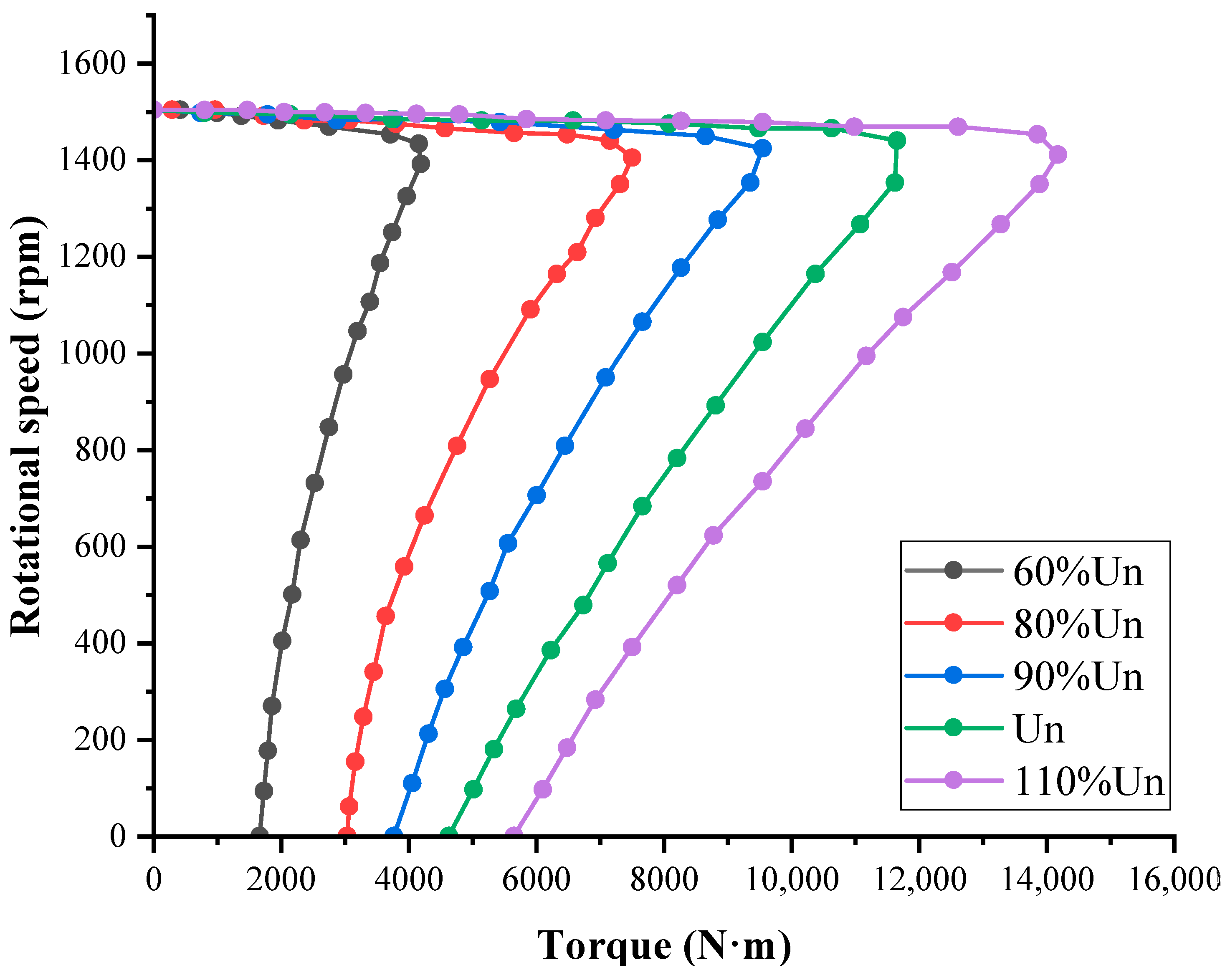
The mud pump exhibited different mechanical characteristics when operated at different voltages. Figure 11 shows the mechanical characteristic curves of the mud pump at rated voltage values of 60%, 80%, 90%, 100%, and 110%.

When the voltage is Un, the relationship between the rotor amplitude and rotational speed is analyzed based on the data of the speed and torque. When the rotational speed is 0 rpm, the displacement of the rotor over time is shown in Figure 12. From the figure, it can be observed that the rotor amplitude is 2.2411 mm. By conducting the same analysis, the amplitude corresponding to each rotational speed on the mechanical characteristic curve can be obtained. The analysis results are shown in Figure 13, indicating that the rotor amplitude increases with an increase in the rotational speed initially, followed by a decrease. For a motor speed between 0 and 1440 rpm, the amplitude increases slowly with an increase in the speed. When the motor speed is between 1440 and 1500 rpm, the amplitude decreases rapidly with an increase in the motor speed. The maximum amplitude of 2.8179 mm was observed at a rotational speed of 1440 rpm. According to the relationship between mud pump torque and rotational speed on the mechanical characteristic curve, the mud pump torque also exhibited an initial increase followed by a decrease with an increase in the rotational speed. Furthermore, both the maximum torque and vibration occurred at a rotational speed of 1440 rpm.

3. Prediction of Pump Amplitude Based on the Support Vector Regression Algorithm

To accurately determine the relationship between the mud pump’s amplitude and input parameters, it was necessary to conduct a predictive analysis of the pump’s amplitude. In this section, the support vector regression (SVR) algorithm is used to predict the amplitude of the mud pump, enabling the prediction of amplitude conditions using a small amount of data on speed, torque, and amplitude.

When using support vector machines for the regression analysis, nonlinear mapping $\mathrm{\Phi }(x)$ was employed to map the input vectors to a high-dimensional feature space. Subsequently, linear regression was performed in the high-dimensional feature space to find the optimal hyperplane that minimized the errors of all samples from the optimal hyperplane.

Assuming the training sample set is $\left\{(x_i,y_i),i=1,2,\cdots ,N\right\}$, where $N$ is the number of samples, $x_i$ represents the input values, and $y_i$ represents the desired output values. The regression model of the SVM can be expressed as the following equation [40]:

$$f(x)=w\times \mathrm{\Phi }(x)+b$$

(6)

where $w$ and $b$ are the weight vector and bias, respectively. Introducing the penalty factor $c$ and slack variables ${\xi }_i(1=1,2,\cdots ,N)$ under the insensitive loss function $\epsilon$, the solution of the SVR is an optimization problem.

$$\left\{\begin{array}{l}\underset{w,b}{\min }\frac{1}{2}{‖w‖}^2+c{\displaystyle \sum _{i=1}^N({\xi }_i+{\xi }_i^{*})}\\ s.t\left\{\begin{array}{l}{y}_i-w\cdot \mathrm{\Phi }(x)-b\le \epsilon +{\xi }_i\\ y_i-w\cdot \mathrm{\Phi }(x)-b\ge -\epsilon -{\xi }_i{}^{*}\end{array}\right.\\ {\xi }_i,{\xi }_{{}_i}^{*}\ge 0,(i=1,2,\cdots ,N)\end{array}\right.$$

(7)

By introducing the Lagrange multiplier $\left\{{\alpha }_i,{\alpha }_i^{*},{\beta }_i,{\beta }_i^{*},(i=1,2,\cdots ,N)\right\}$, Equation (7) can be rewritten as Equation (8):

$$\begin{array}{l}\underset{w,b}{\min }L(w,b,\xi ,{\xi }^{*})=\frac{1}{2}{‖w‖}^2+c{\displaystyle \sum _{i=1}^N({\xi }_i+{\xi }_{{}_i}^{*})}\\ -{\displaystyle \sum _{i=1}^N{\alpha }_i\left[\epsilon +{\xi }_i-y_i+w\cdot \mathrm{\Phi }(x_i)+b\right]}\\ -{\displaystyle \sum _{i=1}^N{\alpha }_{{}_i}^{*}\left[\epsilon +{\xi }_{{}_i}^{*}+y_i-w\cdot \mathrm{\Phi }(x_i)-b\right]}\\ -{\displaystyle \sum _{i=1}^N\left({\beta }_i{\xi }_i+{\beta }_{{}_i}^{*}{\xi }_{{}_i}^{*}\right)}\end{array}$$

(8)

By taking the partial derivatives of $W$, $b$, ${\xi }_i$, and ${\xi }_i^{*}$ in Equation (8), the following can be obtained:

$$\left\{\begin{array}{l}\frac{\partial L}{\partial w}=w-{\displaystyle \sum _{i=1}^N({\alpha }_i-{\alpha }_{{}_i}^{*})\cdot \mathrm{\Phi }(x)=0}\\ \frac{\partial L}{\partial b}=-{\displaystyle \sum _{i=1}^N({\alpha }_i-{\alpha }_{{}_i}^{*})=0}\\ \frac{\partial L}{\partial {\xi }_i}=c-{\alpha }_i-{\beta }_i=0\\ \frac{\partial L}{\partial {\xi }_{{}_i}^{*}}=c-{\alpha }_{{}_i}^{*}-{\beta }_{{}_i}^{*}=0\end{array}\right.$$

(9)

By substituting Equation (9) into Equation (8), the dual form of Equation (7) can be obtained:

$$\begin{array}{l}\underset{\alpha ,{\alpha }^{*}}{\max }{\displaystyle \sum _{i=1}^N({\alpha }_i-{\alpha }_{{}_i}^{*})y_i-}{\displaystyle \sum _{i=1}^N({\alpha }_i+{\alpha }_{{}_i}^{*})\epsilon }\\ -\frac{1}{2}{\displaystyle \sum _{i=1}^N{\displaystyle \sum _{j=1}^N({\alpha }_i-{\alpha }_{{}_i}^{*})({\alpha }_j-{\alpha }_{{}_j}^{*})}}\mathrm{\Phi }(x_i)\mathrm{\Phi }(x_j)\\ s.t.{\displaystyle \sum _{i=1}^N({\alpha }_i-{\alpha }_{{}_i}^{*})=0}\\ {\alpha }_i\ge 0,{\alpha }_{{}_i}^{*}\le c,(i=1,2,\cdots ,N)\end{array}$$

(10)

By introducing the kernel function $K(x_i,x_j)=\mathrm{\Phi }(x_i)\mathrm{\Phi }(x_j)$, the data are mapped from a low-dimensional space to a high-dimensional space, thereby transforming the linearly inseparable problem into a linearly separable problem. This allows for the calculation of inner products in the high-dimensional space to be performed as function calculations in the low-dimensional space. By employing quadratic programming methods, the optimal solution $({\alpha }_i,{\alpha }_{{}_i}^{*})$ for Equation (11) can be obtained, resulting in the decision function of the SVR:

$$f(x)={\displaystyle \sum _{i=1}^N({\alpha }_i-{\alpha }_{{}_i}^{*})K(x_i,x_j)+b}$$

(11)

Due to the advantages of high accuracy and low computational complexity, the radial basis function (RBF) is employed for training and prediction. It is defined as:

$$K(x_i,x_j)=\exp (-\gamma {‖x_i-x_j‖}^2)$$

(12)

where $\gamma$ is the undetermined kernel parameter. The prediction results are evaluated using the mean relative error (MRE), mean absolute error (MAE), mean squared error (MSE), root mean squared error (RMSE), and coefficient of determination (R²).

The amplitude prediction process is illustrated in Figure 14, and the specific steps are as follows:

Step 1: Construct the training and testing sets. From the given n data samples, select N data samples as the training set. The remaining (n − N) test samples are used as the testing set.

Step 2: Normalize the data samples. The ‘mapminmax’ function is used to normalize the data samples to the range of [−1, 1] to improve the convergence speed and accuracy of the SVR.

Step 3: Parameter optimization. The Gaussian radial basis kernel function is used for training and prediction. The grid search method combined with ten-fold cross-validation is employed to find the optimal penalty factor $c$ and kernel parameter γ. The training set is randomly divided into ten subsets, with nine subsets as the training set and one subset as the validation set. The training and validation sets iterate alternately for ten rounds. In each iteration, the ‘svmtrain’ function is used to train the prediction model, and the RMSE $e_i$ of the prediction model is recorded. The average value $E_i=\frac{1}{10}{\displaystyle \sum _{i=1}^{10}{e}_i}$ is calculated. Then, change the parameters, traverse the grid to train the model for m rounds, and obtain the average RMSE E_m of each round of training. Obtain the minimum value of E_m and determine the optimal parameters of the model.

Step 4: Find out the predicted results. Train the predictive model with the optimal parameters and use the model to predict the output values for the (n − N) test samples, obtaining the model’s output values.

The parameter settings for the SVR algorithm are presented in

Table 5. SVR algorithm parameter settings.

Values of Penalty Factor C	[−10, 0.5, 10]
Values of kernel parameter γ	[−10, 0.5, 10]
Number of cross-validation folds v	5
Training set	50
Testing set	10

. The input data for the amplitude prediction based on the SVR algorithm is shown in Appendix A. The results of the amplitude prediction based on the SVR algorithm are displayed in Figure 15, demonstrating a close match between the actual and predicted values. This indicates a high level of reliability in the prediction results.

4. Conclusions and Recommendations

Based on the study of the relationships among the reverse torque, vibration, and input parameters of the mud pumps in the riserless mud recovery drilling, the following conclusions can be drawn:

(1)

The error between the theoretical calculation and the actual simulation of the reverse torque of the mud pump is inevitable, and the average relative error obtained from the experiments in this paper is only 3.41%, which is within the permissible range.

(2)

When the speed of the mud pump is 0 rpm, the reverse torque of the mud to the pump is the lowest, at −320.4 N·m, and when the speed of the mud pump is 1500 rpm, the reverse torque of the mud to the pump is the highest, at 3620.28 N·m. As the speed of the mud pump increases, the reverse torque of the mud to the pump also increases, which is in line with the actual working condition.

(3)

The amplitude of the mud pump exhibits a pattern of initially increasing and then decreasing with an increase in speed. In the range of 0–1440 rpm, the amplitude increases slowly with the speed. When the motor speed is in the range of 1440–1500 rpm, the amplitude decreases rapidly with an increase in speed. At a speed of 1440 rpm, the amplitude reaches its maximum value of 1.5499 mm. The variation of the rotor amplitude with speed is consistent with the variation of torque with speed in the mechanical characteristics curve of the mud pump.

(4)

The SVR algorithm is applied to predict the amplitude of the mud pump and the predicted values closely match the actual values, which indicates a high level of reliability in the prediction results. The prediction results provide a reference for the stability of the mud pump.