Closed-Loop Current Stimulation Feedback Control of a Neural Mass Model Using Reservoir Computing

Abstract

Transcranial electrical stimulation (tES) is a non-invasive neuromodulatory technique that alters ongoing neural dynamics by injecting an exogenous electrical current through the scalp. Although tES protocols are becoming more common in both clinical and experimental settings, the neurophysiological mechanisms through which tES modulates cortical dynamics are unknown. Most existing tES protocols ignore the potential effect of phasic interactions between endogenous and exogenous currents by stimulating in an open-looped fashion. To better understand the mechanisms of closed-loop tES, we first instantiated a two-column Jansen and Rit model to simulate neuronal dynamics of pyramidal cells and interneurons. An echo-state network (ESN) reservoir computer inverted the dynamics of the model without access to the internal state equations. After inverting the model dynamics, the ESN was used as a closed-loop feedback controller for the neural mass model by predicting the current stimulation input for a desired future output. The ESN was used to predict the endogenous membrane currents of the model from the observable pyramidal cell membrane potentials and then inject current stimulation to destructively interfere with endogenous membrane currents, thereby reducing the energy of the PCs. This simulation approach provides a framework for a model-free closed-loop feedback controller in tES experiments.

1. Introduction

The human brain coordinates the activity of billions of neurons to give rise to cognition and perception. Traditional attempts to understand neural mechanisms rely on observing indirect measures of neural activity when a subject performs a carefully designed, controlled cognitive task. Electroencephalography (EEG), which measures voltages on the scalp that reflect the summation of activity of tens of thousands pyramidal cells (PCs) in the cortex [1], provides one common tool for such observations. Many cognitive tasks elicit rich oscillatory EEG dynamics; however, correlative observational studies cannot address whether such patterns in local field potentials (and subsequently EEG) serve a mechanistic purpose or are simply an epiphenomenon not directly related to cognition [2]. To address this issue, experimenters have used neuromodulation to demonstrate a causal role of oscillatory patterns by perturbing neural activity and observing impacts on cognitive behavior [3]. For instance, transcranial electrical stimulation (tES) studies, in which an electric field is injected into the scalp to alter the local field potential, have been shown to affect neural oscillations important in attention [4,5,6] and working memory [7,8].

While tES has contributed to our understanding of neural mechanisms that underlie cognitive processes, both the technology itself and the experimental designs that use tES suffer from important limitations. First and most critically, the way in which tES modulates neural activity and behavior is not clear. Some argue that low intensity, random noise stimulation can bias a neuron to respond when its activity is close to its firing threshold through stochastic resonance [9]. On the other hand, a higher intensity sinusoidal current may cause network entrainment in which external and internal oscillations synchronize [10]. Models of coupled oscillators suggest that the frequency of the externally applied current should match the natural resonance of the internal model to best facilitate entrainment [11,12,13]. However, practical considerations lead many experimenters to opt instead for a simpler, less tailored scheme in which all subjects receive the same fixed-frequency stimulation [14]. This failure to individualize stimulation may lead to inconsistent effects in tES experiments, since resonant frequencies of neural oscillators can vary across subjects for the same cognitive task [15,16]. To further complicate issues, keeping tES electrode placement fixed while ignoring individual anatomical differences can impact the effective strength of the imposed electric field at a targeted brain region [17].

These shortcomings of tES experimental designs can be ameliorated using a closed-loop design, where current stimulation hyperparameters (e.g., stimulation waveform and location) are updated in response to ongoing brain activity [18]. The ideal tES closed-loop setting would utilize rhythmic resonance, which is similar to stochastic resonance; however, in rhythmic resonance excitation is precisely timed to real-time membrane potential recordings to bias a single neuron near the threshold [13]. Non-invasive tES using existing technologies, such as with state-of-the-art targeting algorithms combined with high-definition stimulation electrodes, cannot achieve this. Stimulation spreads widely, across entire gyri, rather than being localized to small subsets of neurons [19,20]. Additionally, though artifact removal algorithms have shown some success in recovering the underlying EEG signal, real-time neural recordings with simultaneous tES still are contaminated by electrical artifacts [21,22]. One closed-loop study attempted to deliver transcranial alternating current stimulation (tACS) in-phase with ongoing alpha oscillations recorded via EEG, but found that alpha amplitude modulation was independent of the endogenous alpha phase, inconsistent with predictions from rhythmic resonance [23]. Closed-loop tACS that matched both frequency and phase of slow-wave oscillations during sleep improved sleep quality compared to a sham condition; however, no open-loop control condition was performed to assess whether this improvement was due to the closed-loop design for the increase in sleep quality [24]. These results hint that closed-loop tES protocols can be effective, but more robust methodologies and controls are needed to produce consistent results.

One way to study mechanisms of closed-loop tES while sidestepping some practical constraints is to investigate neural population behaviors using computational models. Such models avoid complications introduced by human variability and technology limitations to explore more directly how stimulation can affect the brain. The Jansen and Rit neural mass model (JRNMM) [25] provides one platform that lends itself to simulating neural dynamics and how electrical perturbation can shift population behavior. The JRNMM treats a column of cortex as interconnected layers of excitatory interneurons, pyramidal cells and inhibitory interneurons, each of which is modeled by a set of second-order nonlinear differential equations. Because the state variables encode the membrane potentials and currents of each given subpopulation, tES can easily be introduced by adding an independent external current to the internal membrane currents. This approach offers a controlled in silico environment to model neural dynamics under the influence of tES. Closed-loop stimulation can be implemented by observing the output of the JRNMM and providing desired external stimulation calculated using a closed-loop feedback controller.

Closed-loop feedback controllers depend upon system identification to operate. In practice, this can be difficult to achieve due to limited access to internal model states. Some linearization techniques to control nonlinear systems require access to model state equations [26], which may not be possible in a neuroscientific setting where changes in connectivity or anatomy may alter the underlying equations that govern neural interactions. Model-free nonlinear control approaches avoid such a pitfall. One such method uses a time-series prediction scheme using echo-state networks (ESNs) to invert system dynamics by predicting the system output from a given input [27]. The ESN approach can be reversed to perform nonlinear control: the ESN is used to predict the system input that will yield a desired system output [28]. While the ESN model-free approach does not require rigorous linearization techniques, it does require adequate training data for system identification.

To understand how closed-loop current stimulation can modulate neuronal dynamics, we adapted approaches that simulate electrical current stimulation to dynamical models of the brain; this allowed us to modulate endogenous neural oscillations [29,30]. We used a JRNMM to simulate two interacting cortical sources driven by random noise [11,25,31,32]. The objective of our study was to develop a closed-loop controller to control the nonlinear stochastic dynamics of the JRNMM. An echo-state network (ESN) reservoir computer was used to invert the dynamics of the JRNMM, by training the ESN to predict the input that gave rise to the observed dynamics of the PCs of the model. The ESN closed-loop controller was able to suppress the output of the JRNMM even without access to the internal states of the model or any knowledge of the state equations. The ESN controller was able to predict and then destructively interfere with the endogenous membrane currents. These findings demonstrate one possible mechanism for how the phase of current stimulation can impact the modulation of neural oscillations, providing a framework for developing robust, reliable perturbations of neural activity using closed-loop tES.

2. Methods

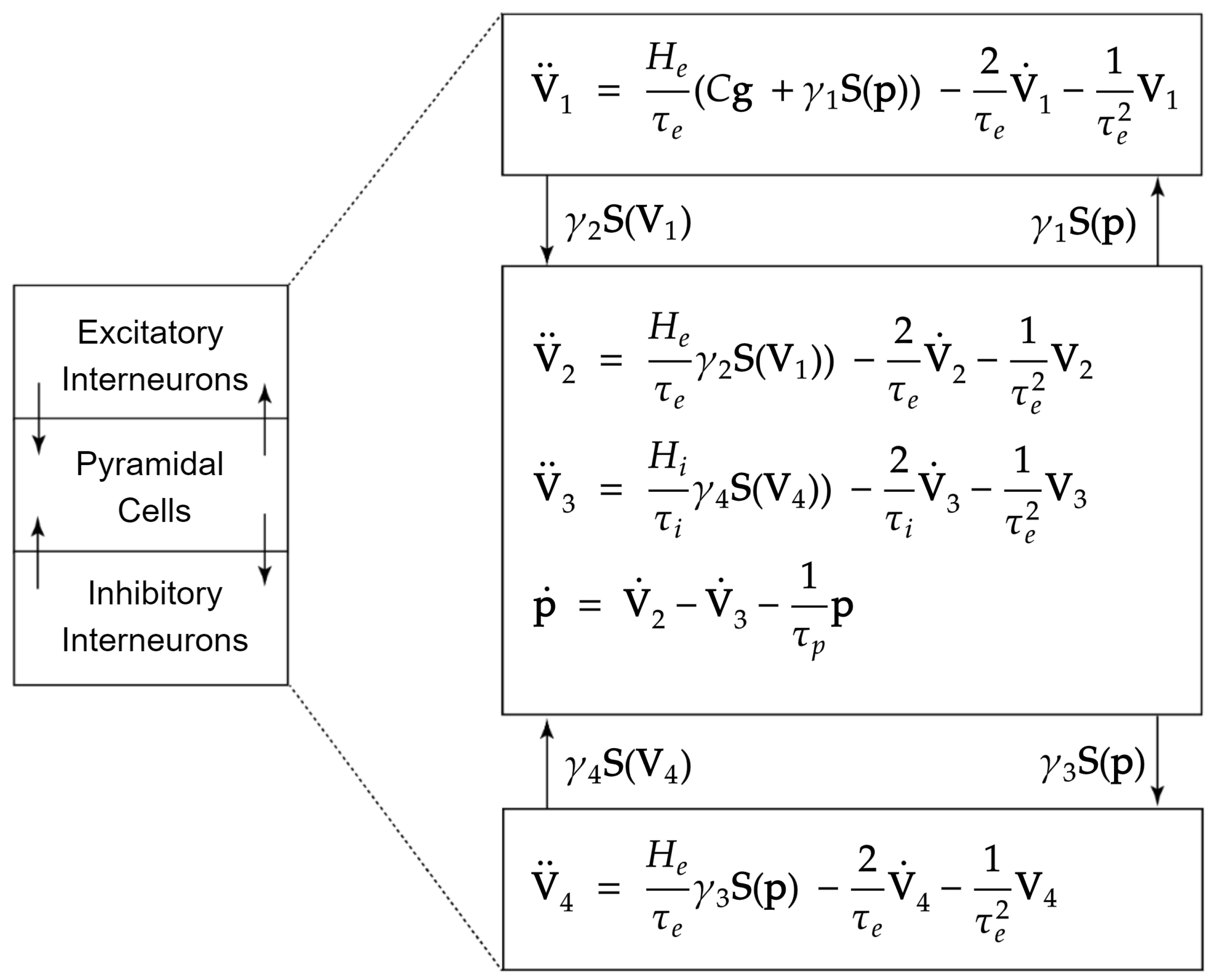
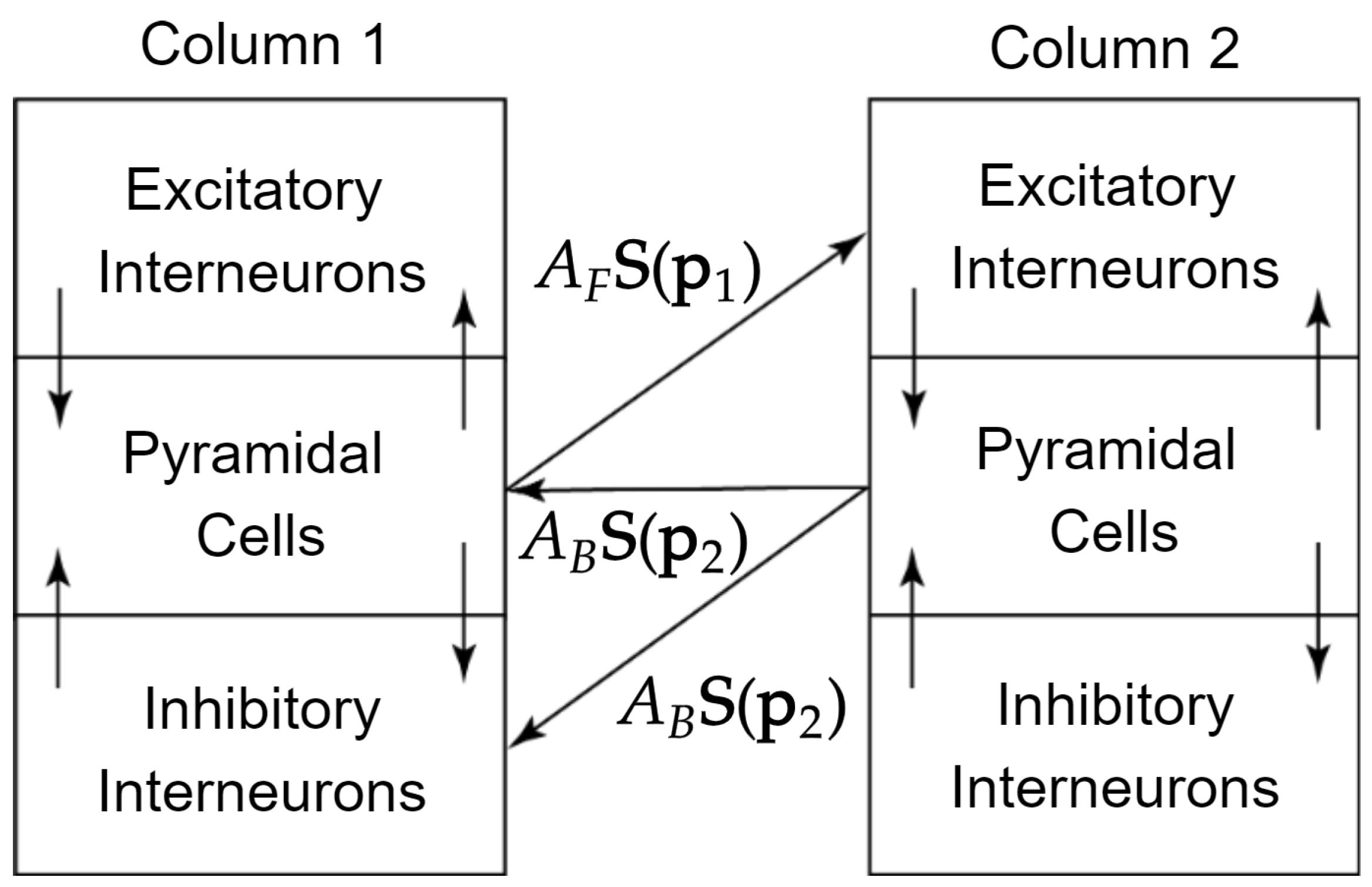
2.1. Jansen and Rit Neural Mass Model

The single-column JRNMM treats a column of cortex as a combination of interconnected excitatory interneurons, pyramidal cells (PCs) and inhibitory interneurons [25]. Each subpopulation has a single state parameter that models the membrane potential of a given subpopulation. A sigmoidal function maps the membrane potential of a subpopulation to a mean firing rate, which then serves as an input to another subpopulation through intrinsic connections. Excitatory interneurons receive a mean firing rate input from both a user-defined external signal $\mathbf{g}$ and inputs from the PC layer. Inhibitory interneurons receive a mean firing rate input from only the PC layer. The PC layer receives inputs from both the excitatory and inhibitory interneurons.

Table 1. Description of model parameters.

Parameter	Description	Value
$H_e,H_i$	Max amplitude of post-synaptic potential	3.25, 29.3 (mV)
${\tau }_e,{\tau }_i,{\tau }_p$	Lumped time constants of dendritic delays	10, 15, 20 (${\mathrm{s}}^{-1}$)
$e_0$	Max firing rate of neural population	2.5 (${\mathrm{s}}^{-1}$)
$r_0$	Steepness of the sigmoid function	0.56 (${\mathrm{mV}}^{-1}$)
${\gamma }_1\dots {\gamma }_4$	Number of synapses in neural population	50, 40, 12, 12
C	Connectivity scalar for extrinsic inputs	1000

and Figure 1 contain the parameters and a diagram of the single-column JRNMM. Appendix A details the full state equations. We modified the JRNMM described in [31] by subtracting the membrane potential $\mathbf{p}$, from the first time derivative of $\mathbf{p}$ to remove DC offsets that would persist after current stimulation, to allow us to only observe perturbations around baseline. The sigmoid function $\mathbf{S}(·)$ converts membrane potentials from other populations into a firing rate, which serves as an input to another population:

$$\mathbf{S}\left({\mathbf{V}}_j\right)=\frac{2e_0}{1+\mathbf{exp}(-r_0{\mathbf{V}}_j)}-e_0$$

(1)

The single-column JRNMM can be easily expanded to include multiple interacting neural mass models with extrinsic connections between populations [31]. In a two-column model, the PCs from one column drive the subpopulations in the other column (Figure 2). Forward connections are excitatory and represent a bottom-up influence, which adds a firing rate input to the excitatory interneurons of the other cortical column. Backward connections provide top-down inhibition that increases the firing rate input to the depolarizing potential of the PC layer and inhibitory interneurons of the other cortical column.

The parameters $A_F$ and $A_B$ parameterize the strength of the forward and backward connections from the other column, which has state equations of a similar form. Specifically, these values represent the average number of synaptic connections formed between the two columns. The PC membrane potentials of columns 1 and 2 are ${\mathbf{p}}_1$ and ${\mathbf{p}}_2$, respectively. The PC inputs between columns contain a delay to simulate conduction delays, here set to 0.01 ms. The two-column JRNMM allows the user to explore richer dynamics, as well as functional and effective connectivity between columns. The EEG signal is dominated by the activity of PCs (because they generate currents orthogonal to the scalp); therefore, ${\mathbf{p}}_1$ and ${\mathbf{p}}_2$ serve as the observable outputs of the model. In our simulations, we set forward connections from column 1 to column 2 with strength $A_F=5$ and backward connections from column 2 to column 1 with strength $A_B=20$. The input $\mathbf{g}$ was random noise pulse density with zero mean and variance of 0.05 spikes per second. The model was implemented in Matlab Simulink by integrating the state equations. The power spectral densities (PSDs) of the PCs were calculated using a multi-taper FFT using the Fieldtrip toolbox [33].

In vivo current stimulation applies an external electrical field to modulate neuronal dynamics. The external electric field is thought to affect PCs predominantly, given that their electric fields are oriented orthogonal to the scalp [10]. Current stimulation can be applied to the JRNMM model by adding the external current to the endogenous current

$$\dot{\mathbf{p}}={\dot{\mathbf{V}}}_{\mathbf{2}}-{\dot{\mathbf{V}}}_{\mathbf{3}}-\frac{1}{{\tau }_p}\mathbf{p}+\mathbf{I}$$

(2)

where $\mathbf{I}$ is the current stimulation to the model, since the first time derivative of voltage is proportional to the membrane current and the constant of proportionality is the membrane capacitance [13].

2.2. Echo State Networks for Nonlinear Control

Reservoir computers are a class of time-series prediction models often used in conjunction with dynamical systems to predict the output signal given an input signal [27]. Put loosely, a reservoir can be thought of as a set of oscillators that are linearly combined to predict the output signal. Because the reservoirs are fixed and only a single output layer is trained, reservoir computers are less susceptible to vanishing gradients caused by back propagation through deep networks, making them relatively stable during fitting. Reservoir computers have also been applied in the context of nonlinear control to predict the input signal given a future output signal [28,34]. After training the reservoir computer, the modeler can then set a desired future output signal and predict the input that should be applied to achieve the desired future output as a function of time. One advantage of using reservoir computers for nonlinear control is that the user does not need access to the internal state equations of the dynamics, but only the input and output signals. Using an echo-state network (ESN) for the choice of reservoir, the internal dynamics $\mathbf{x}\left(n\right)$ are calculated from input $\mathbf{u}\left(n\right)$ and output $\mathbf{y}\left(n\right)$:

$$\begin{array}{c}\mathbf{x}(n+1)=\mathbf{tanh}\left({\mathbf{W}}_{\mathbf{in}}\mathbf{u}(n+1)+\mathbf{W}\mathbf{x}\left(n\right)+{\mathbf{W}}_{\mathbf{back}}\mathbf{y}\left(n\right)\right)\\ \mathbf{y}(n+1)={\mathbf{W}}_{\mathbf{out}}\left[\mathbf{u}(n+1),\mathbf{W}\mathbf{x}(n+1),{\mathbf{W}}_{\mathbf{back}}\mathbf{y}\left(n\right)\right]\end{array}$$

(3)

where $\mathbf{u}\left(n\right)$ is the input signal, $\mathbf{x}\left(n\right)$ are the internal dynamics of the reservoir and $\mathbf{y}\left(n\right)$ is the output signal; these are all time-series vectors. The reservoir parameters ${\mathbf{W}}_{\mathbf{in}},{\mathbf{W}}_{\mathbf{back}}$ and $\mathbf{W}$ are fixed, while the parameters ${\mathbf{W}}_{\mathbf{out}}$ are calculated by concatenating

$$\left[\mathbf{u}(n+1),\mathbf{x}(n+1),\mathbf{y}\left(n\right)\right]$$

(4)

into a single vector, followed by linear regression.

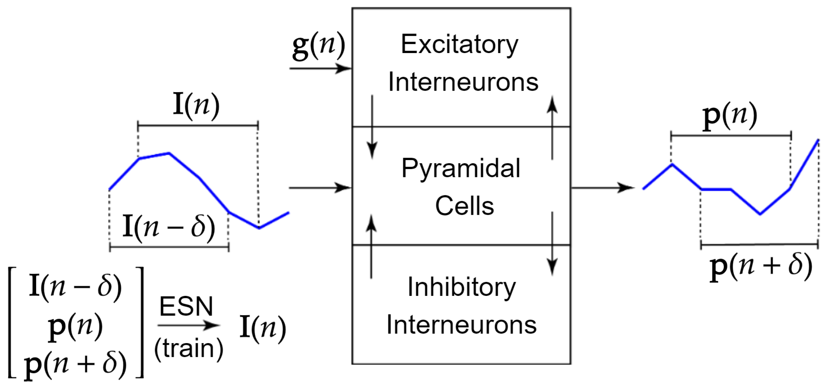
2.3. Current Stimulation Input Prediction

Reservoir computers have been often used as a forward prediction method to predict the output of a dynamical system given an input. In this study, we aimed to invert our neural dynamical system by predicting the input for a desired future output. Then, after training a network to invert our system, we can set the future desired output to be zero and the network would return the input that would drive the system output state to zero. In the context of the JRNMM, the objective is to predict the current input that gives a desired set of PC potentials. We followed an approach similar to [28], where the ESN predicts the current stimulation input $\mathbf{I}\left(n\right)$ given the current PC dynamics $\mathbf{p}\left(n\right)$ and the future dynamics $\mathbf{p}(n+\delta )$ for a time step $\delta$ (which the model has access to since the ESN is trained offline). We also found that including the previous current stimulation $\mathbf{I}(n-m\delta )$ for m number of previous time points improved training and testing accuracy.

2.4. Training Set Generation

For the rest of the paper, we use the notation $\mathbf{X}\left(\mathbf{n}\right)$ to denote a vector time-series $\mathbf{X}$ that ends at time n. Each signal $\mathbf{I}\left(n\right)$, $\mathbf{I}(n-\delta )$, $\mathbf{p}\left(n\right)$, $\mathbf{p}(n+\delta )$ has dimensions ${\mathbb{R}}^{2\times 60}$, where 2 corresponds to the number of columns (i.e., $\mathbf{p}$ is a concatenation of ${\mathbf{p}}_1$ and ${\mathbf{p}}_2$) and 60 is the number of samples. Signal $\mathbf{I}(n-\delta )$ is a delayed copy of $\mathbf{I}\left(n\right)$, delayed by the time step $\delta$, which was set to 0.01 s. The time sample size 60 (taken with a sampling period of 0.01 s) was chosen to capture one full cycle of frequencies greater than 1.67 Hz, which we found to be adequate to capture the model dynamics since the peak model frequency was around 5 Hz. The resulting input to the ESN $\mathbf{u}\left(n\right)$ was a concatenation of $\mathbf{I}(n-\delta )$, $\mathbf{p}\left(n\right)$, $\mathbf{p}(n+\delta )$ to yield a signal with size ${\mathbb{R}}^{6\times 60}$. The output signal predicted by the ESN $\mathbf{y}\left(n\right)$ was set to be $\mathbf{I}\left(n\right)$, the current stimulation input to be applied that led to the future dynamics $\mathbf{p}(n+\delta )$. A schematic describing the prediction procedure can be seen in Figure 3.

To invert the dynamics of the JRNMM, the ESN must observe a sufficient number of $\mathbf{I}\left(n\right)$ current stimulations and corresponding $\mathbf{p}\left(n\right)$ PC dynamics. To do so, we developed the following paradigm to generate various current stimulation inputs to the model. For each of the two PC layers in each of the columns, the current input $\mathbf{I}\left(n\right)$ was white noise with a noise power of 0.1 (height of the power spectral density). The noise was then bandpass filtered between 0.1 and 30 Hz. To allow for the ESN to observe both onset and offsets of current stimulation, the resulting bandpass filtered noise was multiplied by a unit amplitude pulse function. The pulse function had a period uniformly drawn from $[0.1,0.2,\dots ,1]$ seconds. The pulse had a width of $[10,20,\dots ,90]$ percent of the period, also uniformly drawn. Each pulse started with a time delay of 0.5 s. The pulse was then multiplied by a gain uniformly drawn from $[1,2,\dots ,10]$. Figure 4 shows a sample current stimulation input. The simulation was run 1000 times at a sampling period of 0.001 s with a simulation duration of 4 s, then downsampled to a sampling period of 0.01. Each iteration had randomized current inputs $\mathbf{I}\left(n\right)$ across all iterations and PC layers, as well as randomized $\mathbf{u}\left(n\right)$ inputs to the excitatory interneurons.

2.5. Training Parameters

The resulting input data set $\mathbf{U}$ with dimensions $(1000\times 6\times 400)$, corresponding to 1000 independent trials; the sum of the two PC potentials, two delayed PC potentials and two delayed current stimulations (one for each PC layer); and 400 time points, respectively. The output data set $\mathbf{Y}$ had dimensions $(1000\times 2\times 400)$, corresponding to 1000 trials, the current stimulation for each of the PC layers and the 400 time points. Each trial was segmented into non-overlapping 60-time-point windows, to give a total of 6000 trials. Of this total, 4800 trials were randomly selected for training, while the remaining 1200 were reserved as a test set. The ESN was trained using the parameters described in

Table 2. Echo state network parameters. The notations ${\mathbf{n}}_{\mathbf{in}}$ and ${\mathbf{n}}_{\mathbf{out}}$ correspond to a vector with all entries n with length equal to the number of input and output units, respectively. Scaling and shifting correspond to element-wise multiplication or addition between the scaling/shifting vector and the data input vector. It is often desirable for data to be centered near zero, depending on the nonlinear activation function being used.

Parameter	Value
Spectral radius	0.5
N input units	6
N internal units	10
Input scaling	${\mathbf{1}}_{\mathbf{in}}$
Input shift	${\mathbf{0}}_{\mathbf{in}}$
Teacher scaling	$\mathbf{0}.{\mathbf{1}}_{\mathbf{out}}$
Teacher shift	${\mathbf{0}}_{\mathbf{out}}$
Feedback scaling	$\mathbf{0}.{\mathbf{1}}_{\mathbf{in}}$

and we briefly explored a few additional ESN parameters in Appendix B. To explore the effect of the training set size, the amount of training data was varied while keeping the number of testing data points fixed. We averaged five random initializations to generate the final ESN prediction.

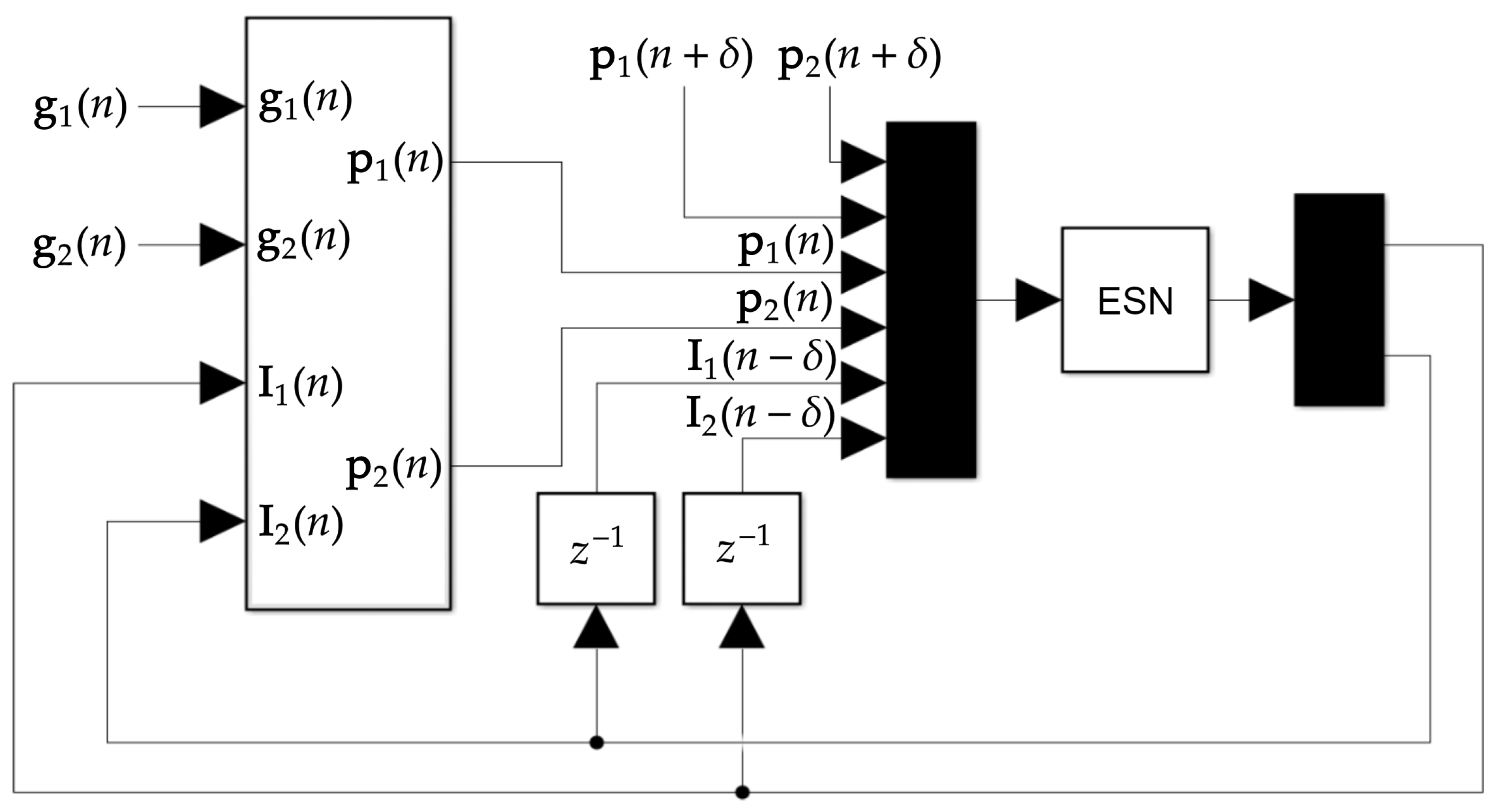
2.6. Closed-Loop Feedback Loop Using the ESN

The ESN predicts the current stimulation input $\mathbf{I}\left(n\right)$ that should be injected into the PC layer to achieve the desired PC dynamics $\mathbf{p}(n+\delta )$ given $\mathbf{p}\left(n\right)$ and the stimulation history $\mathbf{I}(n-\delta )$. In this study, we aimed to achieve PC layer outputs equal to zero, corresponding to suppressing activity in a cortical region. Ideally, one could simply find the externally applied current that drives $\mathbf{p}(n+\delta )=0$. However, because the stochastic input $\mathbf{u}\left(n\right)$ is constantly driving the dynamics of the JRNMM, the PC output can never be held at zero. Indeed, we found that setting the desired output to $\mathbf{p}(n+\delta )=0$ led to instability in the controller. To achieve better stability, we instead encouraged the future PC output to tend towards zero, by setting $\mathbf{p}(n+\delta )=k\mathbf{p}\left(n\right)$, where $k\in (0,1)$ is a hyperparameter explored in this study. A schematic of the controller can be seen in Figure 5.

2.7. ESN Performance Metrics

The mean-squared error (MSE) for the train and test sets was used to evaluate the performance of the ESN. Only the last time point predicted by the ESN, averaged over both PCs, was used when calculating the MSE. We used this approach because the overlap of the input and output signal otherwise could have caused confounds in training performance. The MSE of the PC output was measured to determine how well the ESN closed-loop feedback controller suppressed the energy of the PC across both columns. This MSE was compared to the model without any feedback, as well as a random control: injecting the current stimulation $\mathbf{I}\left(n\right)$ selected from an iteration with a different noise input. We also compared the power spectral density of the PC output from these three conditions.

3. Results

3.1. Model Output

Figure 6 shows the output of a single trial of the simulation, without any feedback control, for both of the PC columns. The time series of the membrane potential shows stochastic activity bounded between −0.5 and 0.5 mV. The PSD shows a unimodal spectrum for both columns with a peak at around 5–6 Hz.

3.2. Feedback Results

For the remainder of the results, only the output from PC column 1 is shown, as the outputs from PC column 2 are similar, but with an overall smaller magnitude. The mean-squared error for ESN training and testing is shown in Figure 7 for different log fractions of the training data used while keeping the amount of testing data fixed. Interestingly, even though the MSE became more stable as the amount of training data increased, it did not reduce testing MSE (in Figure 7, the blue training data MSE fluctuates when the amount of training data is small, even though the test set MSE is similar, regardless of the amount of training data used). This point is considered in more detail below.

We explored the extent to which the ESN feedback controller could suppress the model output (the PC column values). Figure 8 shows the mean-squared membrane potential of PC column 1 with feedback using the input current predicted to inhibit the output, no feedback, or mismatched feedback control taken from a different random run of the model, each taken over 100 trials. For each of the random trials, appropriate feedback led to the smallest PC output and random feedback produced the largest. This observation was supported by statistical analysis using a repeated measures ANOVA test, which found a significant effect on the type of feedback stimulation (F(2, 198) = 313.97, p < 0.001).

To explore the effect of the hyperparameter k on the energy suppression of the model, we ran the simulation for various values of k and different log fractions of the training data. Figure 9 shows the average percent change in energy of PC column 1 compared to the no-feedback condition for the different values of k and log fractions of the training data over all trials. The choice of k greatly impacted the degree to which the PC output was suppressed, but the output energy was less strongly affected by the amount of training data provided to the model. Specifically, as seen in Figure 9, values of k less than about 0.9 led to increases in output energy. The output energy decreased as k increased within each row. However, output energy was relatively similar within a given column. That said, even though different amounts of training data led to similar suppression of the PC output, it greatly affected the feedback current used to suppress the output, both in the total energy and the power spectra of the control signal, as shown in Figure 10. Increasing the amount of training data caused the ESN to learn more efficient, lower energy current inputs to achieve the same overall suppression. A single trial of the ESN feedback control results can be seen in Figure 11 and the PSD of the PC column 1 averaged over all trials is shown in Figure 12.

To shed light on the mechanisms by which the ESN controller may be suppressing the energy of the PC layer, we calculated the amount of destructive/constructive interference with the endogenous membrane currents $({\dot{\mathbf{V}}}_{\mathbf{1},\mathbf{2}}-{\dot{\mathbf{V}}}_{\mathbf{1},\mathbf{3}})$ and the injected current stimulation ${\mathbf{I}}_1$. Indeed, Figure 13. shows that the injected current destructively interferes with the endogenous membrane currents. A paired t-test found that the endogenous membrane current plus the ESN feedback was lower than the endogenous current by itself (t = 8.033, p < 0.001).

4. Discussion

Interest in tES as a neuromodulatory technique is growing in medical and experimental settings, even though the mechanisms through which tES operates continue to be debated. Most published tES studies stimulate on a timescale of tens of minutes, using narrowband inputs whose stimulation frequency matches the resonant frequency of the targeted neural network [3]. However, there are other important considerations in tES experimental design beyond matching a brain region’s resonant frequency. Carefully timing the phase onset of tES to align with ongoing neural oscillations has measurable perceptual effects [35]. Such results support the notion that closed-loop tES protocols guided by real-time neural signature recordings could achieve more robust and predictable outcomes [18]. This line of work is still in the early stages of development due to challenges in tES artifact removal in neural recordings to validate successful neuromodulation [21], subject variability (which can alter tES effects) [17] and challenges in designing a stable closed-loop controller [23].

To address these issues, we first developed a computational platform to study oscillatory dynamics of a neural system by instantiating a two-column JRNMM [25,31]. This model simulated two connected cortical sources through a set of nonlinear second-order differential equations with membrane potentials as the state variables. tES was simulated by injecting external current into the membrane currents of the PC layer of the model. This provided us with a closed-loop framework: simulated EEG recordings could be “recorded” from the PC layer of the model while also being stimulated by exogenous electrical current. Because latent variables and state equations cannot be observed in most neuroscientific settings, we adapted a model-free method to design a feedback controller for this nonlinear stochastic dynamical system. Specifically, we used an ESN reservoir computer as a time-series prediction model. We then inverted the dynamics of the model by predicting the appropriate current stimulation input to achieve a desired output of the model based on observing the previous outputs of the PC layer [27,28]. In this work, we only explored one set of parameters for the JRNMM. A potential future development would be to test the effectiveness of the ESN across multiple different parameters to yield different neural mass dynamics and different neural mass models [36].

Upon being driven by random noise, the baseline JRNMM PCs generate an output with a broad-band spectra with a unimodal peak around 5 Hz (the resonant frequency of our model, given our parameter choices). Both columns 1 and 2 showed similar spectra; however, column 1 (whose PCs fed back to the excitatory interneurons in column 2; see Figure 2) always had greater power than column 2 (whose PCs fed back to column 1’s PCs and inhibitory neurons). The ESN was trained by injecting randomized current into the model and using the subsequent PC output as the input to the ESN. The current injection was used as the output of the ESN, which caused the ESN to predict the current input that gave rise to the observed PC output. We varied the amount of training data used in order to assess how ESN performance would be affected in real-world settings where data are likely limited. We found that even with very limited training data (the lowest amount being 132 trials, which corresponded to around 80 s of stimulation data), the total output was reduced by about the same amount as when we used the full training data set (1 h of stimulation data). Given that some tES protocols are on the order of tens of minutes [5], acquisition of adequate amounts of data should be possible in practice, though the noise acquired in realistic settings may impede ESN training. The fact that the ESN dynamics could be learned with a small amount of training data may indicate that the state equations behave in a nearly linear fashion. Since the only nonlinearity in the model was from the sigmoidal function that converts membrane potentials into firing rates, it could mean that the model was operating near the linear part of the sigmoid function.

The closed-loop controller was implemented after the ESN network was trained. During the training period, the ESN was fed the current PC output and the future PC output to predict the stimulation current to deliver in order to reduce future PC output. In the closed-loop feedback setting, the ESN was also fed the current PC output, but the future PC output had to be manually set based on the desired dynamics at the next time step. We found that setting the future PC output to be a scaled down version of the current PC output resulted in a closed-loop controller that stably suppressed the energy output of the PCs. In a perfect setting, the future PC output would be equated to zero to drive the dynamics to zero energy. However, this caused the model to become unstable. This was most likely due to the stochastic noise constantly input into the model, which prevented the model from being held at zero energy. We explored the effect of different values of the scaling parameter k on the amount of energy suppression in the PC layer and found that scaling parameters in the range of 0.9 to 1 resulted in the greatest amount of energy suppression, while lower values of 0.7 to 0.8 increased the energy of the PC layer. The optimal choices of scaling parameter k and training set size reduced the energy output of PC layer 1 by around 30%. Varying the amount of training data while keeping the scaling parameter fixed did not significantly impact the amount of energy reduction, but strongly impacted characteristics of the current stimulation. Specifically, the ESN controller learned more efficient, lower energy current stimulation feedback with more training data.

The ESN controller suppressed PC energy by predicting and subsequently destructively interfering with endogenous membrane currents, demonstrating that the feedback controller successfully estimated internal states of the model from the observable PC output. It may have been the case that the ESN learned an internal representation of phase space of the endogenous currents, similar to the models in [37,38]. Providing additional features of the data (e.g., instantaneous phase or wavelet coefficients) could assist the ESN in learning this phasic representation. Because the controller successfully estimated the internal membrane currents, simply switching the sign of the injected current would positively reinforce ongoing dynamics. This approach could potentially be applied in both human or animal models by first identifying a target dipole source using source localization techniques, then modeling current flow using forward models [39]. Current source density methods could also be used to estimate the radial current flow at the scalp [40]. After estimating the current over the entire scalp, tES could be applied in an open-loop setting to destructively interfere with the estimated current. The closed-loop method proposed in this paper could be performed on real-time EEG data, given a successful tES removal artifact algorithm that could operate in real time. Alternatively, if one relaxed the requirement of performing ongoing current stimulation, EEG could be recorded in short windows without stimulation, alternating with intermittent tES, to avoid artifacts [41].

5. Summary

A Jansen and Rit neural mass model was used to simulate closed-loop current stimulation. An echo-state network, used to invert the dynamics of the stochastic nonlinear neural mass model, successfully predicted current stimulation inputs to modulate the dynamics of the model. The controller implicitly estimated the endogenous membrane currents of the model and subsequently could be used to successfully modulate output currents. This approach provides a potential framework for delivering closed-loop current stimulation to the brain.

References

1. Teplan, M. Fundamentals of EEG Measurement. Meas. Sci. Rev. 2002, 2, 1–11. [Google Scholar]
2. Thut, G.; Miniussi, C.; Gross, J. The Functional Importance of Rhythmic Activity in the Brain. Curr. Biol. 2012, 22, R658–R663. [Google Scholar] [CrossRef] [Green Version]
3. Herrmann, C.S.; Rach, S.; Neuling, T.; Strüber, D. Transcranial alternating current stimulation: A review of the underlying mechanisms and modulation of cognitive processes. Front. Hum. Neurosci. 2013, 7, 279. [Google Scholar] [CrossRef] [PubMed] [Green Version]
4. Kasten, F.H.; Wendeln, T.; Stecher, H.I.; Herrmann, C.S. Hemisphere-specific, differential effects of lateralized, occipital-parietal α-versus γ-tACS on endogenous but not exogenous visual-spatial attention. Sci. Rep. 2020, 10, 12270. [Google Scholar] [CrossRef] [PubMed]
5. Deng, Y.; Reinhart, R.M.; Choi, I.; Shinn-Cunningham, B. Causal links between parietal alpha activity and spatial auditory attention. eLife 2019, 8, e51184. [Google Scholar] [CrossRef] [PubMed]
6. Dallmer-Zerbe, I.; Popp, F.; Lam, A.P.; Philipsen, A.; Herrmann, C.S. Transcranial Alternating Current Stimulation (tACS) as a Tool to Modulate P300 Amplitude in Attention Deficit Hyperactivity Disorder (ADHD): Preliminary Findings. Brain Topogr. 2020, 33, 191–207. [Google Scholar] [CrossRef] [Green Version]
7. Reinhart, R.M.; Nguyen, J.A. Working memory revived in older adults by synchronizing rhythmic brain circuits. Nat. Neurosci. 2019, 22, 820–827. [Google Scholar] [CrossRef] [Green Version]
8. Hoy, K.E.; Bailey, N.; Arnold, S.; Windsor, K.; John, J.; Daskalakis, Z.J.; Fitzgerald, P.B. The effect of γ-tACS on working memory performance in healthy controls. Brain Cogn. 2015, 101, 51–56. [Google Scholar] [CrossRef]
9. Geisler, C.D.; Goldberg, J.M. A Stochastic Model of the Repetitive Activity of Neurons. Biophys. J. 1966, 6, 53–69. [Google Scholar] [CrossRef] [Green Version]
10. Liu, A.; Vöröslakos, M.; Kronberg, G.; Henin, S.; Krause, M.R.; Huang, Y.; Opitz, A.; Mehta, A.; Pack, C.C.; Krekelberg, B.; et al. Immediate neurophysiological effects of transcranial electrical stimulation. Nat. Commun. 2018, 9, 5092. [Google Scholar] [CrossRef] [Green Version]
11. Pei, A.; Shinn-Cunningham, B.G. Alternating current stimulation entrains and connects cortical regions in a neural mass model. In Proceedings of the Annual International Conference of the IEEE Engineering in Medicine and Biology Society, EMBS, Glasgow, UK, 11–15 July 2022; pp. 760–763. [Google Scholar] [CrossRef]
12. Huang, W.A.; Stitt, I.M.; Negahbani, E.; Passey, D.J.; Ahn, S.; Davey, M.; Dannhauer, M.; Doan, T.T.; Hoover, A.C.; Peterchev, A.V.; et al. Transcranial alternating current stimulation entrains alpha oscillations by preferential phase synchronization of fast-spiking cortical neurons to stimulation waveform. Nat. Commun. 2021, 12, 3151. [Google Scholar] [CrossRef] [PubMed]
13. Ali, M.M.; Sellers, K.K.; Fröhlich, F. Transcranial alternating current stimulation modulates large-scale cortical network activity by network resonance. J. Neurosci. 2013, 33, 11262–11275. [Google Scholar] [CrossRef]
14. Veniero, D.; Benwell, C.S.; Ahrens, M.M.; Thut, G. Inconsistent effects of parietal α-tACS on Pseudoneglect across two experiments: A failed internal replication. Front. Psychol. 2017, 8, 952. [Google Scholar] [CrossRef] [Green Version]
15. Mioni, G.; Shelp, A.; Stanfield-Wiswell, C.T.; Gladhill, K.A.; Bader, F.; Wiener, M. Modulation of Individual Alpha Frequency with tACS shifts Time Perception. Cereb. Cortex Commun. 2020, 1, 1–9. [Google Scholar] [CrossRef]
16. Gulbinaite, R.; Van Viegen, T.; Wieling, M.; Cohen, M.X.; Vanrullen, R. Individual Alpha Peak Frequency Predicts 10 Hz Flicker Effects on Selective Attention. J. Neurosci. 2017, 37, 10173. [Google Scholar] [CrossRef] [Green Version]
17. Kasten, F.H.; Duecker, K.; Maack, M.C.; Meiser, A.; Herrmann, C.S. Integrating electric field modeling and neuroimaging to explain inter-individual variability of tACS effects. Nat. Commun. 2019, 10, 5427. [Google Scholar] [CrossRef] [PubMed] [Green Version]
18. Thut, G.; Bergmann, T.O.; Fröhlich, F.; Soekadar, S.R.; Brittain, J.S.; Valero-Cabré, A.; Sack, A.T.; Miniussi, C.; Antal, A.; Siebner, H.R.; et al. Guiding transcranial brain stimulation by EEG/MEG to interact with ongoing brain activity and associated functions: A position paper. Clin. Neurophysiol. 2017, 128, 843–857. [Google Scholar] [CrossRef] [PubMed] [Green Version]
19. Dmochowski, J.P.; Datta, A.; Bikson, M.; Su, Y.; Parra, L.C. Optimized multi-electrode stimulation increases focality and intensity at target. J. Neural Eng. 2011, 8, 046011. [Google Scholar] [CrossRef] [PubMed]
20. Wu, L.; Liu, T.; Wang, J. Improving the Effect of Transcranial Alternating Current Stimulation (tACS): A Systematic Review. Front. Hum. Neurosci. 2021, 15, 255. [Google Scholar] [CrossRef]
21. Neuling, T.; Ruhnau, P.; Weisz, N.; Herrmann, C.S.; Demarchi, G. Faith and oscillations recovered: On analyzing EEG/MEG signals during tACS. NeuroImage 2017, 147, 960–963. [Google Scholar] [CrossRef]
22. Kohli, S.; Casson, A.J. Removal of Transcranial a.c. Current Stimulation artifact from simultaneous EEG recordings by superposition of moving averages. In Proceedings of the Annual International Conference of the IEEE Engineering in Medicine and Biology Society, EMBS, Milan, Italy, 25–29 August 2015; pp. 3436–3439. [Google Scholar] [CrossRef] [Green Version]
23. Zarubin, G.; Gundlach, C.; Nikulin, V.; Villringer, A.; Bogdan, M. Transient Amplitude Modulation of Alpha-Band Oscillations by Short-Time Intermittent Closed-Loop tACS. Front. Hum. Neurosci. 2020, 14, 366. [Google Scholar] [CrossRef] [PubMed]
24. Robinson, C.S.; Bryant, N.B.; Maxwell, J.W.; Jones, A.P.; Robert, B.; Lamphere, M.; Combs, A.; Al Azzawi, H.M.; Gibson, B.C.; Sanguinetti, J.L.; et al. The Benefits of Closed-Loop Transcranial Alternating Current Stimulation on Subjective Sleep Quality. Brain Sci. 2018, 8, 204. [Google Scholar] [CrossRef] [PubMed] [Green Version]
25. Jansen, B.H.; Rit, V.G. Electroencephalogram and visual evoked potential generation in a mathematical model of coupled cortical columns. Biol. Cybern. 1995, 73, 357–366. [Google Scholar] [CrossRef] [PubMed]
26. Calvet, J.P.; Arkun, Y. Feedforward and Feedback Linearization of Nonlinear Systems and Its Implementation Using Internal Model Control (IMC). Ind. Eng. Chem. Res. 1988, 27, 1822–1831. [Google Scholar] [CrossRef]
27. Jaeger, H. The “Echo State” Approach to Analysing and Training Recurrent Neural Networks-with an Erratum Note 1; German National Research Center for Information Technology GMD Technical Report: Bonn, Germany, 2001; Volume 148, p. 13. [Google Scholar]
28. Canaday, D.; Pomerance, A.; Gauthier, D.J. Model-free control of dynamical systems with deep reservoir computing. J. Phys. Complex. 2021, 2, 035025. [Google Scholar] [CrossRef]
29. Cakan, C.; Obermayer, K. Biophysically grounded mean-field models of neural populations under electrical stimulation. PLoS Comput. Biol. 2020, 16, e1007822. [Google Scholar] [CrossRef] [Green Version]
30. Dutta, A.; Nitsche, M.A. State-space analysis of Hodgkin-Huxley axonal neural mass model during subthreshold high frequency alternating current stimulation. In Proceedings of the International IEEE/EMBS Conference on Neural Engineering, NER, San Diego, CA, USA, 6–8 November 2013; pp. 1100–1103. [Google Scholar] [CrossRef]
31. David, O.; Harrison, L.; Friston, K.J. Modelling event-related responses in the brain. NeuroImage 2005, 25, 756–770. [Google Scholar] [CrossRef]
32. Pei, A.; Shinn-Cunningham, B.G. Effects of Broadband, Bandstop and Amplitude-Modulated Alternating Current Stimulation on a Neural Mass Model. In Proceedings of the 2022 IEEE Biomedical Circuits and Systems Conference (BioCAS), Taiwan, China, 13–15 October 2022; pp. 284–287. [Google Scholar] [CrossRef]
33. Oostenveld, R.; Fries, P.; Maris, E.; Schoffelen, J.M. FieldTrip: Open source software for advanced analysis of MEG, EEG, and invasive electrophysiological data. Comput. Intell. Neurosci. 2011, 2011, 156869. [Google Scholar] [CrossRef]
34. Haluszczynski, A.; Räth, C. Controlling nonlinear dynamical systems into arbitrary states using machine learning. Sci. Rep. 2021, 11, 12991. [Google Scholar] [CrossRef]
35. Neuling, T.; Rach, S.; Wagner, S.; Wolters, C.H.; Herrmann, C.S. Good vibrations: Oscillatory phase shapes perception. NeuroImage 2012, 63, 771–778. [Google Scholar] [CrossRef]
36. Grimbert, F.; Faugeras, O. Bifurcation analysis of Jansen’s neural mass model. Neural Comput. 2006, 18, 3052–3068. [Google Scholar] [CrossRef] [PubMed]
37. Matsuda, T.; Komaki, F. Time series decomposition into oscillation components and phase estimation. Neural Comput. 2017, 29, 332–367. [Google Scholar] [CrossRef] [PubMed]
38. Wodeyar, A.; Schatza, M.; Widge, A.S.; Eden, U.T.; Kramer, M.A. A state space modeling approach to real-time phase estimation. Elife 2021, 10, e68803. [Google Scholar] [CrossRef]
39. Michel, C.M.; Brunet, D. EEG source imaging: A practical review of the analysis steps. Front. Neurol. 2019, 10, 325. [Google Scholar] [CrossRef] [PubMed] [Green Version]
40. Kayser, J.; Tenke, C.E. On the benefits of using surface Laplacian (Current Source Density) methodology in electrophysiology. Int. J. Psychophysiol. Off. J. Int. Organ. Psychophysiol. 2015, 97, 171. [Google Scholar] [CrossRef] [Green Version]
41. Castellano, M.; Ibañez-Soria, D.; Kroupi, E.; Acedo, J.; Campolo, M.; Soria-Frisch, A.; Valls-Sole, J.; Verma, A.; Ruffini, G. Intermittent tACS during a visual task impacts neural oscillations and LZW complexity. Exp. Brain Res. 2020, 238, 1411–1422. [Google Scholar] [CrossRef]
Figure 1. Single-column Jansen and Ritt neural mass model. The state V j describes the membrane potential of the jth subpopulation ( j = 1 excitatory interneurons membrane potential, j = 2 PC depolarizing membrane potential, j = 3 PC hyperpolarizing membrane potential, j = 4 inhibitory interneuron membrane potential). The net PC depolarization is p . Reproduced from [11] with permission.
Applsci 13 01279 g001
Figure 2. Two-column Jansen and Ritt neural mass model. The PC depolarization from each column is converted to an extrinsic firing rate input to the other column.
Applsci 13 01279 g002
Figure 3. The current stimulation I ( n ) is injected into the JRNMM to yield the PC dynamics p ( n ) . The previous inputs I ( n δ ) , along with the current and future dynamics p ( n ) and p ( n + δ ) were used to predict the input I ( n ) which gave rise to the future dynamics. Random noise g ( n ) is also input into the excitatory interneurons. Only one cortical column is shown; however, this process is carried out on the two-column model.
Applsci 13 01279 g003
Figure 4. Sample current signal with units mA, proportional up to a constant C representing the capacitance of the membrane, injected into the JRNMM for both PC column 1 (blue) and column 2 (red).
Applsci 13 01279 g004
Figure 5. Closed loop feedback control schematic for the ESN. g 1 ( n ) and g 2 ( n ) are the white noise inputs driving PC column 1 and 2, respectively. The PC outputs p 1 ( n ) and p 2 ( n ) are concatenated along with the previous current stimulation inputs I 1 ( n δ ) and I 2 ( n δ ) , as well as the desired dynamics p 1 ( n + δ ) and p 2 ( n + δ ) . The trained ESN then predicts the current stimulation input I 1 ( n ) and I 2 ( n ) that should be injected into the model to achieve the desired dynamics.
Applsci 13 01279 g005
Figure 6. A single trial of the simulation without feedback control. (A) The time series output of the PCs for two seconds of the simulation. The blue trace indicates column 1, while the red trace indicates column 2. (B) PSD of the membrane potentials for both of the column’s PCs calculated using a multitaper FFT.
Applsci 13 01279 g006
Figure 7. Mean-squared training and testing error (with units mA up to a constant of proportionality related to membrane potential) calculated from the last data point predicted from the ESN output averaged over both PC columns, plotted against different log fractions of the training data.
Applsci 13 01279 g007
Figure 8. Mean squared membrane potential ( mV 2 ) of PC column 1 for 100 trials. FB = Feedback from ESN, Rand FB = Feedback from a different random seed, No FB = no ESN feedback. The results above are shown for the ESN network trained on all of the data (log fraction of the data = 1) and with a value of k = 1 .
Applsci 13 01279 g008
Figure 9. Percentchange in PC output energy relative to the no-feedback condition: 100   × (energy with feedback − energy without feedback)/energy without feedback. Data are shown for different values of k and log fractions of the training data. Positive values correspond to increases in the PC output energy and negative values to (desired) decreases with injected current feedback. More training data did not impact the amount of energy reduction as much as the desired-dynamics parameter k. Setting k to be less than about 0.9 caused the model to increase overall PC energy output rather than suppressing PC energy output.
Applsci 13 01279 g009
Figure 10. (A) Mean energy of the current stimulation learned by the ESN for different amounts of training data. (B) Mean PSD of the current stimulation for different log fractions of training data. More training data resulted in the feedback controller to learn more efficient current stimulation inputs.
Applsci 13 01279 g010
Figure 11. Single trial of the ESN feedback controller. Each of the plots correspond to the PC column 1 output. (A) PC column 1 membrane potential with feedback, feedback from a different random seed and no feedback. The controller feedback begins at two seconds. (B) PSD of the three conditions of PC column 1. (C) Current stimulation predicted output from the ESN controller. (D) PSD of the current stimulation output. The PSD is proportional up to a constant C, the capacitance of the membrane. The results above are shown for the ESN network trained on all of the data (log fraction of the data = 1) and with a value of k = 1 .
Applsci 13 01279 g011
Figure 12. PSD of PC column 1 averaged over 100 trials. Shaded regions denote ± 1 standard error of the mean. The results above are shown for the ESN network trained on all of the data (log fraction of the data = 1) and with a value of k = 1 .
Applsci 13 01279 g012
Figure 13. (A) Single trial showing the endogenous membrane current (red) and the endogenous membrane current + the ESN current feedback (blue). Adding the ESN current feedback destructively interfered with the ongoing currents. (B) The mean squared membrane current without the feedback and with the feedback for all 100 trials. The results above are shown for the ESN network trained on all of the data (log fraction of the data = 1) and with a value of k = 1 .
Applsci 13 01279 g013