Abstract
Stochastic configuration network (SCN) is a mathematical model of incremental generation under a supervision mechanism, which has universal approximation property and advantages in data modeling. However, the efficiency of SCN is affected by some network parameters. An optimized searching algorithm for the input weights and biases is proposed in this paper. An optimization model with constraints is first established based on the convergence theory and inequality supervision mechanism of SCN; Then, a hybrid bat-particle swarm optimization algorithm (G-BAPSO) based on gradient information is proposed under the framework of PSO algorithm, which mainly uses gradient information and local adaptive adjustment mechanism characterized by pulse emission frequency to improve the searching ability. The algorithm optimizes the input weights and biases to improve the convergence rate of the network. Simulation results over some datasets demonstrate the feasibility and validity of the proposed algorithm. The training RMSE of G-BAPSO-SCN increased by and compared with that of SCN in the two regression experiments, and the recognition accuracy of G-BAPSO-SCN increased by 0.07% on average in the classification experiments.
1. Introduction
Randomized algorithms have the characteristics of fast learning and show great potential in machine learning [1,2,3]. These algorithms generally select the input parameters randomly and then calculate the output parameters based on the least square method. There are many categories of random weight networks. In addition to the typical feedforward neural network, there are also recurrent neural networks with random weights and randomized kernel approximations [4].
At the beginning, most randomized weights networks could not determine the appropriate number of hidden nodes. To solve this problem, the incremental learning algorithm was proposed. The network gradually increases the hidden nodes until the tolerance is reached. This method optimizes the network structure and avoids the waste of hidden nodes. Based on this idea, SLFNN, which has approximation properties, was proposed by Kwok et al [5]. They also adopted a modified Quickprop algorithm to update the network weights. The random Vector Function Link (RVFL) network also used the incremental strategy to build its structure, which probabilistically converges when the input side parameters of the network are appropriately selected [6,7]. Otherwise, the convergence can not be guaranteed [8]. In 2009, Tyukin I proposed that the RVFL network needed a supervision mechanism, and they verified that the RVFL network could not approximate a given objective function through the experiments [9]. Subsequently, this phenomenon had been further proved mathematically [10]. The proposal of SCN solves the problem that the network did not have universal approximation property [8]. SCN used an inequality constraint mechanism to allocate input parameters randomly and expanded the selection range of random parameters adaptively, so as to ensure the approximation of the established stochastic learning network. It was an incremental generative network, and the input parameters were stochastically configurated under the inequality constraint, and the output parameters were determined by constructional method or by solving the least square problem. Subsequently, SCN based on the depth model was also proposed, and depth SCN still has universal approximation properties under the inequality supervision mechanism [11]. At present, SCN has been successfully applied to underground airflow quantity modeling, ball mill load condition recognition, sewage quality index estimation, and nonlinear system intelligent modeling [12,13,14,15].
The universal approximation property of SCN is an advantage that other randomized learning techniques do not have, as the adaptive search algorithm of the weights and biases tries to keep the parameters in a small range as possible. However, the output weights are usually large, so the generalization performance of the network is affected. Overall, the optimization of SCN focuses on the following aspects: first, improving the generalization performance, for instance, and norm regularization methods based on SCN are proposed respectively to avoid the risk of the model overfitting [13,15]. The partial least squares method is used to calculate the output parameters, replacing the ordinary least squares method [14]. In addition, the famous negative correlation learning method could evaluate the output side parameters based on the SCN mode. The Block Jacobi and Gauss–Seidel methods are used to solve the output weights of ill-posed equations iteratively based on heterogeneous feature groups, in which the convergence analysis is given and the uniqueness of these iterative solutions is proved [16]. The second aspect is to optimize the generation mode of the network; some scholars have proposed to change the incremental mode of the hidden nodes in the process of SCN construction, and the incremental mode of hidden nodes was improved from single incremental to block incremental [17,18]. The third aspect is to optimize the hyperparameters of the network. In the discussion of the input weights, some scholars indicate that the method based on the inequality supervision mechanism to search weights leads to a certain rejection rate, therefore, the conditions of inequality constraints should be relaxed, so as to improve the acceptance rate of the random value and reduce the number of iterations for the searching of input weights [19]. However, the accuracy of the network will be reduced once the inequality constraints are relaxed, which has a certain cost. Some scholars also focus on regularization parameters and scale factors of weights and bias that affect the network performance, and optimize them using a chaotic sparrow search algorithm, which makes the network achieve better performance [20]. Meanwhile, some scholars also applied various feedback learning mechanisms to optimize SCN [21,22].
There are few studies on how to optimize the input side parameters directly. SCN searches the input side parameters randomly until the parameters could satisfy the inequality constraints. The specific method is to expand the search interval gradually linearly, and randomly generate a large number of weights and biases in the interval to judge whether the inequality constraints are satisfied, then select the best one. The method will affect the efficiency of SCN. Therefore, an efficient optimization algorithm needs to be designed. The gradient descent method is often used to solve optimization problems in practical engineering, that is, to solve for a minimum in the direction of gradient descent or to solve for a maximum in the direction of gradient ascent. However, this method is easy to fall into the local minimum for non-convex optimization problems, so it needs to be combined with an intelligent optimization algorithm to achieve better performance [23,24]. The bat algorithm [25,26] and Particle Swarm Optimization (PSO) algorithm [27] are population-based stochastic optimization technical algorithms, which seek the optimal solution by imitating the group behavior of the biological world. The bat algorithm is a search algorithm to simulate the predation behaviors of bats, which has been successfully applied to microgrid scheduling [28], harmful plants classification [29], text categorization [30], and the categorization salesman problem [31]. These algorithms could search more regions in the solution space of the objective function simultaneously, which is flexible and easy to implement, and requires fewer parameters to be adjusted. In addition, the gradient information could be used to determine the search direction because of the randomness of intelligent optimization algorithms. Therefore, using the hybrid optimization algorithm to search the input parameters of SCN could optimize the network structure and improve the convergence speed.
This paper focuses on improving the search algorithm for the input weights and biases. In order to accelerate the convergence speed, an optimization model was established based on the inequality constraint mechanism by analyzing the convergence principle of SCN. Then, an improved optimization algorithm (G-BAPSO) is proposed, which combines the gradient information of the objective function and searches for the optimal weights and biases using the hybrid PSO and bat algorithm. Finally, an optimized stochastic configuration network based on the G-BAPSO algorithm is established.
The structure of this paper is as follows: The theory of SCN is introduced in Section 2; G-BAPSO-SCN is proposed in Section 3, including the optimization model and algorithm. In Section 4, the G-BAPSO algorithm is verified on some benchmark functions, and the performance of G-BAPSO-SCN and other models is compared in some regression and classification problems. The experimental results are analyzed in Section 5, and Section 6 gives the conclusion of this paper.
2. Preliminaries
2.1. Stochastic Configuration Network
SCN has been a powerful data modeling tool in recent years. The model is incrementally generated by stochastic configuration algorithms, which performs well in classification and regression problems and has the ability of universal approximation. The structure of SCN is shown in Figure 1, where x denotes the input data, s denotes the activation function, and f denotes the output of network.

Figure 1.
The structure of SCN with a hidden layer.
For the dataset , and the corresponding output datasets , . If nodes have been configured on the network, the outputs of L-th node in the hidden layer is calculated by Formula (1)
where h stands for the activation function, and is the weight and bias of the first layer. The weights of the second layer is calculated by the least squares algorithm, as shown in Formula (2).
where stands for the q-th error of the network output when there are already nodes in the hidden layer. stands for the q-th output of SCN, which is calculated by Formula (4), and the error of SCN with L-nodes is shown in Formula (5).
and need satisfy the supervision mechanism (7).
where stands for the upper bound of the activation function, is a sequence that goes to zero, and r is a regularization parameter close to 1. Hidden nodes are added in this sequence until the model reaches the tolerance, that is, when the error between the model outputs and target outputs reaches the preset threshold, the structure, weight, and threshold parameters of the SCN are determined, then the learning process stops. It has been proved mathematically that the model has universal approximation capability, namely . Principles and Formulas (1)–(8) of SCN are from Ref. [8].
The specific search algorithm for the input weights and biases of SCN is as follows.
Step 1. Set the sequence of interval length for searching the parameters,
;
Step 2. Generate a set of random values in the interval , then judge whether it satisfies the inequality constraint or not;
Step 3. If there are parameters satisfying the inequality constraints, the parameters that could maximize (Formula (9)) are selected to configure the new hidden node. Otherwise, expand the search interval to , and repeat the above steps until the tolerance is reached [8].
2.2. Particle Swarm Optimization Algorithm and Bat Algorithm
PSO is an iterative algorithm based on the simulation of the foraging process of birds. Firstly, the population is randomly initialized, including the position and velocity of the individual. Secondly, we calculate the fitness of each particle to obtain the initial optimal solution of each particle. Thirdly, the velocity and position are updated by Formulas (11) and (12) in each iteration until the solution meets the conditions.
where stands for the velocity of the individual at time t, stands for the location of the individual at time t, and stand for the individual extremum and global extremum, respectively, at time t. and are learning factors, and are random numbers.
The bat algorithm is a heuristic search algorithm to simulate the predation behaviors of bats. The bats constantly adjust the positions to determine the optimal solution according to the unique frequency, wavelength, and loudness. It has simple model and fast convergence speed. However, the optimization accuracy of the algorithm is low. It is based on the following assumptions: Firstly, all bats could sense distance by echolocation, and distinguish targets and obstacles in a special way; Secondly, bats fly randomly at the location with the speed , search for targets with loudness, frequency, and variable wavelength, and adjust the wavelength (or frequency) and pulse emission rate automatically by the distance from the target; Thirdly, the loudness gradually decreases from to [32].
The updated formulas of frequency, speed, and position are as follows:
where stands for the frequency of the i-th bat, its adjustment range is , , is the current optimal solution.
Generates a random number for the current local search field. If , update the value of p by Formula (16).
where , stands for the average loudness of bats at time t.
The loudness drops to a fixed value as the bat approaches its target, then continues to increase. Generate a random number , if and , is accepted, namely . The loudness and the pulse emission rate are updated under the Formulas (17) and (18).
where and , and stand for the loudness and pulse emission rate of the i-th bat at time t, respectively.
3. G-BAPSO-SCN
3.1. Establish the Optimization Model
According to the convergence principle of SCN [8], taking the difference between the error of the model with hidden nodes and the error of the model with L hidden nodes as the objective function is beneficial to directly improve the convergence rate of the model. The larger the is, the faster the network convergence rate is. Therefore, the optimization configuration of the input parameters is transformed into solving the following optimization problem under the constraint of inequality (20). is a continuous function, and the convergence speed of the network could be improved when the input weights and biases are configured by the solutions of the optimal problem (21).
3.2. Solve the Optimization Problem Based on the G-BAPSO Algorithm
The input parameters are generated randomly in SCN, and the selected range will gradually and linearly expand to search the random parameters that meet the criteria (7). In order to make the search algorithm more flexible and speed up the convergence, this section is devoted to improving the algorithm of the input weights and biases. If the network output is 1-dimensional (same for multi-dimensional output), according to the Cauchy Schwartz inequality , equal is true when and are linearly dependent, and the function could be maximized. However, it is obviously impossible to find consistent and linear correlation for different inputs, and the non-convexity of the function is obvious, so it is not feasible to find the theoretical optimal solution by the gradient descent method. Therefore, an intelligent optimization algorithm combined with gradient information should be considered to optimize the objective function.
3.2.1. Calculate the Gradient Information
The gradient direction plays an important role in the search process. Calculate the gradient based on the objective function (21). The results are shown in Formulas (22)–(25), where d stands for the features of the input samples, m stands for the output dimension, N stands for the number of samples, and L stands for the hidden node.
3.2.2. G-BAPSO Algorithm
The G-BAPSO algorithm introduces the local search mechanism and adaptive individual elimination strategy of the BAT algorithm under the framework of PSO. When the pulse frequency is low and the current individual fitness is less than the average fitness, Formula (16) is used to update the local individual position. Otherwise, individual velocity is updated by combining gradient information in the process of global search. With the guidance of gradient direction, the search speed is accelerated; the search mechanism of the bat-PSO algorithm could fully explore the solution space and help to jump out of the local minimum.
The combination of the two could improve the search efficiency. The global update formula is shown in Formulas (26)–(28), where grad represents the gradient and is a learning factor. The specific description of the G-BAPSO algorithm is shown in Algorithm 1, and the flow chart is presented in Figure 2.
where grad represents the gradient and is the learning factor.
| Algorithm 1: The G-BAPSO algorithm |
|
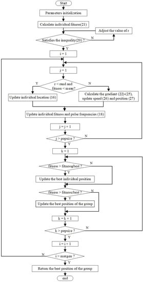
Figure 2.
The flow chart of G-BAPSO.
Set as the maximum number of hidden layer nodes. Under the G-BAPSO algorithm, the optimized configuration algorithm of SCN, called ’G-BAPSO-SC’, is shown in Algorithm 2.
| Algorithm 2: The G-BAPSO-SC algorithm |
|
4. Numerical Experiments
4.1. Evaluation of the G-BAPSO Algorithm
In order to illustrate the efficiency of G-BAPSO, four benchmark functions (29)–(32) are selected to evaluate its performance, and the minimum value of each function is zero. The G-BAPSO algorithm is used to optimize these functions, and it will be compared with Gradient-based PSO (GPSO), PSO, bat, and FOA algorithm. The error of the optimal solution is used as an evaluation index for comparison.
Continuous functions are selected as the benchmark functions in this section because the objective function proposed in Section 2 is multivariate continuous functions. is multi-peak function and the rest are concave function. The graphs of the four functions are shown in Figure 3, Figure 4, Figure 5 and Figure 6. Figure 3 and Figure 6 show the graphs of binary functions corresponding to and , respectively.
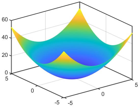
Figure 3.
The figure of function .

Figure 4.
The figure of function .
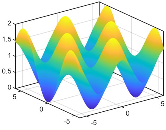
Figure 5.
The figure of function .
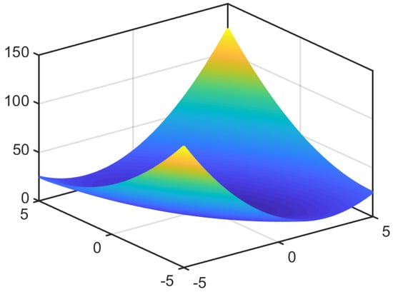
Figure 6.
The figure of function .
Popsize, , , and the number of iterations have an important influence on the G-BAPSO algorithm. In order to determine the optimal value, Refs. [33,34] suggested that and should be 2. Refs. [35,36] conducted sensitivity analysis on popsize, , and other parameters of acceleration. Based on the benchmark test function f1, the sensitivity analysis of relevant parameters of GBAPSO is shown in Table 1, Table 2 and Table 3, and the parameters used in other experiments also follow this method.

Table 1.
The sensitivity analysis of , and popsize.
Table 2.
The sensitivity analysis of .
Table 3.
The sensitivity analysis of the iterations.
Table 1 shows the comparison results of the minimum values of the function f1 when , and popsize are changing. It can be seen that when , and are fixed, the larger the popsize, the smaller the error. However, the order of magnitude of the error only changes slightly as the population size increases to 75 or 100, and the larger the popsize, the longer the calculation time consumed by the algorithm. Therefore, it is necessary to select an appropriate value that can balance the calculation time and error. Fifty is selected as the population number in solving the minimum value of . When the popsize and are fixed, the smaller the and are, the smaller the error will be. When and drop to 0.3, the magnitude of the error has reached , which is within the acceptable range. Table 2 shows the sensitivity analysis for . As increases from 0.2 to 0.8, the error tends to increase first and then decrease. This is because the BAPSO algorithm plays a major role in the algorithm when is very small, and the gradient descent algorithm plays a major role when becomes large. When the value of is near 0.4, there is a balance between the two, which also verifies the effectiveness of the hybrid algorithm. Table 3 shows the sensitivity analysis for the iterations. As the iterations increases, the error of the optimal solution becomes smaller and smaller. However, the more iterations, the greater the time cost. It can be seen that when iterations are 20, the error has reached the magnitude of , which is within the acceptable range.
Table 4 shows the parameter Settings. The program was written on MATLAB R2019a and run on 8G memory and 1.6 Ghz CPU. Each algorithm was independently run 200 times. The experimental results are shown in Table 5.
Table 4.
Parameters setting.
Table 5.
The average error of the optimal solution in 200 experiments.
It can be seen from the results of four groups of experiments that G-BAPSO performs well. Compared with PSO, bat, and FOA, the optimal solution has a significant advantage in order of magnitude. It is worth noting that the performance of G-PSO is comparable to that of G-BAPSO when gradient information is introduced into PSO, indicating that gradient factors are relatively important for these four functions, especially concave functions with obvious characteristics, and it is easy to find the optimal solution quickly according to the gradient direction search. Therefore, the first two algorithms are more efficient than the last three algorithms. When comparing the first two algorithms, one can observe that G-BAPSO performs well because it adds a local search and adaptive elimination strategy of the bat algorithm, which can improve the convergence speed of the algorithm. Note that the error of G-BAPSO and G-PSO for is zero, which means the error is very small, approaching zero.
4.2. Performance of SCN Based on the G-BAPSO Algorithm
In order to illustrate the performance of SCN based on the G-BAPSO algorithm, four groups of numerical simulation experiments are used in this section. We include two groups of classification problems and two groups of regression problems: the problem of function regression, synchronous motor excitation current, identification of bank notes, and the iris data set.
4.2.1. Dataset Information
Dataset 1 is generated by function , , 1000 points are randomly collected as the training set, and the test set is 300 equidistant points on the interval [9].
Dataset 2 is the current data (SM) [37,38] in the UCI database. The task is to find the nonlinear relationship between synchronous motor excitation current and the input features including power factor, load current, synchronous motor excitation current change, and power factor error. There are 557 groups of samples, where 400 samples are used as the training set and 157 samples are used as the test set.
Dataset 3 is the Banknote authentication dataset in the UCI database, which is extracted from images of samples of real and counterfeit bills. The task is to verify the authenticity of bills (classification). The data contains 4 input features (the variance, the skewness, the curtosis, and the entropy of the image), and the output corresponding to each group of input features is the banknote category (true or false). The dataset has 1372 samples, where 1038 samples are used for training and 334 samples are used for testing.
Dataset 4 is the Iris dataset in the UCI database. There are three categories of Iris, and the task is to identify the iris category based on four input attributes including the length and width of calyx, and the length and width of the petal. The dataset contains 150 groups of samples, of which each category contains 50 groups of samples. where 120 groups of samples are used for training and 30 groups of samples are used for testing.
Table 6 shows the relevant information of the four datasets.
Table 6.
Information about the datasets.
4.2.2. Evaluate Metrics and Parameter Settings
Select the sigmoid function as the activation function, as shown in Formula (33). For regression problems, Root mean square error (RMSE) is used as the evaluation index, as shown in Formula (34). The smaller RMSE, the better the network performance. For classification problems, the accuracy rate (ACC) is taken as an evaluation index, as shown in Formula (35). The closer ACC is to 1, the better the network performance is.
where stands for the ideal output of the k-th sample, stands for the network output of the k-th sample. stands for the number of correctly identified samples of class i, and stands for the total sample number of class i.
Based on the above four datasets, G-BAPSO-SCN is compared with SCN [8], RVFL network [7] and ELM [39]. The parameters are shown in Table 7.
Table 7.
Parameters setting for performance test.
4.2.3. The Experimental Results
Due to the influence of random parameters, each group of experiments was run independently for 50 times, and the average results were finally used for the comparative analysis. The convergence curves of the average results of G-BAPSO-SCN and SCN in 50 experiments are drawn in Figure 7, Figure 8, Figure 9 and Figure 10, respectively, and the average running results are shown in Table 8, Table 9, Table 10 and Table 11.
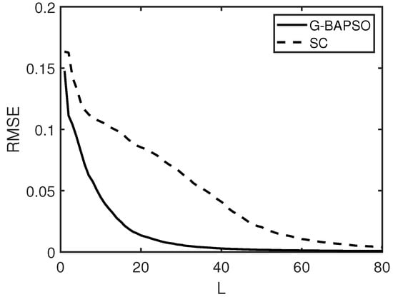
Figure 7.
The average convergence curve (Dataset 1).
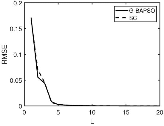
Figure 8.
The average convergence curve (Dataset 2).
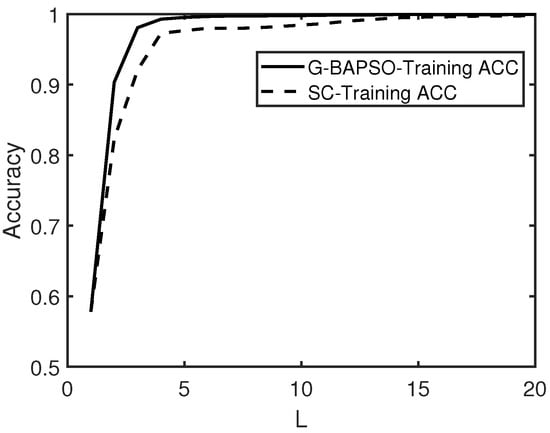
Figure 9.
The average convergence curve (Dataset 3).
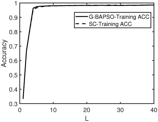
Figure 10.
The average convergence curve (Dataset 4).
Table 8.
Performance comparison results (Dataset 1).
Table 9.
Performance comparison results (Dataset 2).
Table 10.
Performance comparison results (Dataset 3).
Table 11.
Performance comparison results (Dataset 4).
5. Discussion
Table 8, Table 9, Table 10 and Table 11 show that G-BAPSO-SCN converges faster than other models when the number of hidden nodes is the same, and the RVFL network and ELM have relatively poor performance.In regression experiment 1, the training RMSE of G-BAPSO-SCN increased by compared with that of SCN; in regression experiment 2, the training RMSE of G-BAPSO-SCN increased by 0.0032, indicating that the improvement degree of training RMSE not only depends on the algorithm itself, but is also closely related to the distribution characteristics of the data. In classification problems, G-BAPSO-SCN also has an advantage in recognition accuracy, with an average improvement of about 0.07% over SCN. At the same time, it could also be seen from the comparison of convergence curves in Figure 7, Figure 8, Figure 9 and Figure 10 that G-BAPSO-SCN has faster convergence than SCN. Since RVFL and ELM are not incremental generation networks, and their hidden nodes are generated once, the convergence speed between them is not compared with the former two curves.
G-BAPSO-SCN performs well because it introduces a more flexible mechanism in the search of input parameters, allowing it to explore the solution space more thoroughly. The algorithm combines the advantages of the intelligent optimization method and traditional optimization method, and the introduction of gradient makes it possible to approach the optimal solution quickly. By introducing the emission frequency mechanism of bats into the PSO framework, local search could be carried out according to individual fitness and emission frequency at the initial stage, and the poor individuals could be eliminated adaptively, thus accelerating the convergence rate. SCN uses the linear expansion searching method to select the input parameters, which cannot detect the optimal solution with a long distance in the initial stage. The initial configuration is not optimized, thus increasing the searching iterations and the number of nodes to a certain extent. RVFLN is a typical incremental network, so we also compare it with G-BAPSO-SCN. However, RVFLN could not guarantee the convergence, and the accuracy of the network is slightly inferior. ELM’s performance is relatively poor under the same number of hidden nodes as G-BAPSO-SCN. In addition to the optimization of input weights and biases, CSSA-SCN [20] optimizes their search intervals and the regularization factor r of the model, which is the optimization of hyperparameters, and its objective function and optimized parameters are different from those in this paper. Most of the other methods used to optimize SCNS focus on the the output parameters or the generation of model structures.
In conclusion, G-BAPSO-SCN, first proposed in this paper, has a faster convergence rate and a more optimized structure, which can improve the training efficiency of the model and have better performance in the application of regression or prediction.
6. Limitations and Future Works
Table 12 presents the comparison results of the running time of four models based on Dataset 1. It can be seen that G-BAPSO-SCN takes a relatively long time, which is determined by two factors: On the one hand, both G-BAPSO-SCN and SCN are incremental generation models, and the model structure needs to be determined adaptively in the training process, so both of them take a longer time than RVFL and ELM. On the other hand, G-BAPSO-SCN has the search process of the optimal solution based on the hybrid algorithm, and the gradient calculation process obviously increases the time cost. Therefore, in terms of time cost, G-BAPSO-SCN cannot save the training time, which is one of its limitations. However, G-BAPSO-SCN increases the rate of convergence of the model, which is very meaningful for practical problems. Meanwhile, the G-BAPSO algorithm uses some empirical values to initialize the value range (the domain of the objective function) of the input weights and biases, which should be studied and optimized in the future. In addition, other intelligent optimization algorithms can also be used to optimize the input parameters of SCN. The genetic algorithm is also an effective algorithm with fast convergence rate [40], which can be used in the subsequent research.
Table 12.
The comparison of run time based on Dataset 1.
7. Conclusions
The proposed algorithm G-BAPSO provides an alternative solution for improving the convergence speed of SCN. The G-BAPSO algorithm focuses on the search for input weights and biases, considering the gradient information, the global optimal solution, and the individual optimal solution. In the process of searching for the optimal solution. the algorithm adaptively adjusts the local solutions according to the individual emission frequency and fitness in the initial stage. Thus, the convergence speed is improved by combining the traditional optimization algorithm with the intelligent optimization algorithm. At the same time, the algorithm strictly follows the inequality constraint mechanism of SCN, and each optimal solution is generated under the inequality supervision mechanism, which ensures the unique convergence of the SCN network. Numerical experiments also illustrate that SCN based on the G-BAPSO algorithm could be used to solve regression or classification problems. Compared with SCN, the training RMSE of G-BAPSO-SCN increased by and , respectively, and the recognition accuracy of G-BAPSO-SCN increased by 0.07% on average. In industrial applications, the G-BAPSO-SCN proposed in this paper is suitable for nonlinear approximation, regression prediction, and pattern recognition, based on industrial big data.
Author Contributions
Conceptualization, J.L.; methodology, J.L. and Y.L.; software, J.L. and Q.Z.; writing—original draft preparation, J.L.; writing—review and editing, Y.L. All authors have read and agreed to the final version of the manuscript.
Funding
This paper is partly supported by National Science Foundation of China under Grants (62073226), Liaoning Province Natural Science Foundation (2020-KF-11-09, 2022-KF-11-01), Shen-Fu Demonstration Zone Science and Technology Plan Project (2020JH13, 2021JH07), Major Science and Technology Projects of Liaoning Province (2022JH1/10400033), Young Teacher Foundation of Shenyang Institute of Technology (QN202210).
Informed Consent Statement
Informed consent was obtained from all subjects involved in the study.
Data Availability Statement
The data included in this paper are available at http://archive.ics.uci.edu/ml/index.php (accessed on 19 October 2022).
Conflicts of Interest
The authors declare no conflict of interest.
References
- Lukosevicius, M.; Jaeger, H. Reservoir computing approaches to recurrent neural network training. Comput. Sci. Rev. 2009, 3, 127–149. [Google Scholar] [CrossRef]
- Scardapane, S.; Wang, D. Randomness in neural networks: An overview. Wiley Interdiscip. Rev. Data Min. Knowl. Discov. 2017, 7, e1200. [Google Scholar] [CrossRef]
- Wang, D. Editorial: Randomized algorithms for training neural networks. Inf. Sci. 2016, 126–128. [Google Scholar] [CrossRef]
- Rahimi, A.; Recht, B. Advances in Neural Information Processing Systems; MIT Press: Vancouver, BC, Canada, 2007; pp. 1177–1184. [Google Scholar]
- Kwok, T.Y.; Yeung, D.Y. Objective functions for training new hidden units in constructive neural networks. IEEE Trans. Neural Netw. 1997, 8, 1131–1148. [Google Scholar] [CrossRef] [PubMed]
- Igelnik, B.; Pao, Y.H. Stochastic choice of basis functions in adaptive function approximation and the functional-link net. IEEE Trans Neural Netw 1995, 6, 1320–1329. [Google Scholar] [CrossRef]
- Pao, Y.H.; Takefuji, Y. Functional-link net computing: Theory, system architecture, and functionalities. Computer 1992, 25, 76–79. [Google Scholar] [CrossRef]
- Wang, D.; Li, M. Stochastic configuration networks: Fundamentals and algorithms. IEEE Trans. Cybern. 2017, 47, 3466–3479. [Google Scholar] [CrossRef]
- Tyukin, I.; Prokhorov, D. Feasibility of random basis function approximators for modeling and control. In Proceedings of the IEEE Multi-Conference on Systems and Control, Saint Petersburg, Russia, 8–10 July 2009; pp. 1391–1396. [Google Scholar]
- Gorban, A.; Tyukin, I.; Prokhorov, D.; Sofeikov, K.I. Approximation with random bases: Pro etcontra. Inf. Sci. 2016, 364, 129–145. [Google Scholar] [CrossRef]
- Wang, D.; Li, M. Deep stochastic configuration networks with universal approximation property. In Proceedings of the 2018 International Joint Conference on Neural Networks (IJCNN), Rio de Janeiro, Brazil, 8–13 July 2018; pp. 1–8. [Google Scholar]
- Tao, J.; Niu, H.; Zhang, Y.; Li, X. An intelligent modeling method for nonlinear systems based on random Configuration networks. Control Decis. 2022, 37, 2559–2564. [Google Scholar] [CrossRef]
- Wang, Q.; Yang, C.; Ma, X.; Zhang, C.; Peng, S. Underground airflow quantity modeling based on SCN. Acta Autom. Sin. 2021, 47, 1963–1975. [Google Scholar]
- Zhao, L.; Wand, J.; Huang, M.; Wang, G. Estimation of effluent quality index based on partial least squares stochastic configuration networks. CIESC J. 2020, 71, 5672–5680. [Google Scholar]
- Zhao, L.; Zou, S.; Guo, S.; Huang, M. Ball mill load condition recognition model based on regularized stochastic configuration networks. Control. Eng. China 2020, 27, 1–7. [Google Scholar]
- Wang, D.; Cui, C. Stochastic configuration networks ensemble with heterogeneous features for large-scale data analytics. Inf. Sci. 2017, 417, 55–71. [Google Scholar] [CrossRef]
- Dai, W.; Li, D.; Zhou, P. Stochastic configuration networks with block increments for data modeling in process industries. Inform. Sci. 2019, 484, 367–386. [Google Scholar] [CrossRef]
- Tian, Q.; Yuan, S.; Qu, H. Intrusion signal classification using stochastic configuration network with variable increments of hidden nodes. Opt. Eng. 2019, 58, 026105. [Google Scholar] [CrossRef]
- Zhu, X.; Feng, X.; Wang, W. A further study on the inequality constraints in stochastic configuration networks. Inf. Sci. 2019, 487, 77–83. [Google Scholar] [CrossRef]
- Zhang, C.; Ding, S. A stochastic configuration network based on chaotic sparrow search algorithm. Knowl.-Based Syst. 2021, 220, 106924. [Google Scholar] [CrossRef]
- Li, W.; Tao, H.; Li, H. Greengage grading using stochastic configuration networks and a semi-supervised feedback mechanism. Inform. Sci. 2019, 488, 1–12. [Google Scholar] [CrossRef]
- Zhang, Q.; Li, W.; Li, H. Self-blast state detection of glass insulators based on stochastic configuration networks and a feedback transfer learning mechanism. Inf. Sci. 2020, 522, 259–274. [Google Scholar] [CrossRef]
- Momeni, E.; Armaghani, D.J.; Hajihassani, M.; Amin, M.M. Prediction of uniaxial compressive strength of rock samples using hybrid particle swarm optimization-based artificial neural networks. Measurement 2015, 60, 50–63. [Google Scholar] [CrossRef]
- Armaghani, D.J.; Mohamad, E.T.; Narayanasamy, M.S.; Narita, N.; Yagiz, S. Development of hybrid intelligent models for predicting TBM penetration rate in hard rock condition. Tunn. Undergr. Space Technol. 2017, 63, 29–43. [Google Scholar] [CrossRef]
- Gandomi, A.H.; Yang, X.S. Chaotic bat algorithm. J. Comput. Sci. 2014, 5, 224–232. [Google Scholar] [CrossRef]
- Yang, X.S.; Gandoomi, A.H. BAT Algorithm: A Novel Approach for Global Engineering Optimization; Professional Publications: Hyderabad, India, 2012. [Google Scholar]
- Kennedy, J.; Eberhart, R. Particle swarm optimization. In Proceedings of the IEEE Proceedings of ICNN’95—International Conference on Neural Networks, Perth, WA, Australia, 27 November–1 December 1995; pp. 1942–1948. [Google Scholar]
- Whz, A.; Yxw, B.; Yan, Z.C.; Jian, X.C. Research on multi-energy complementary microgrid scheduling strategy based on improved bat algorithm. Energy Rep. 2022, 8, 1258–1272. [Google Scholar]
- Ibrahim, M.H. WBA-DNN: A hybrid weight bat algorithm with deep neural network for classification of poisonous and harmful wild plants. Comput. Electron. Agric. 2021, 190, 106478. [Google Scholar] [CrossRef]
- Eliguzel, N.; Cetinkaya, C.; Dereli, T. A novel approach for text categorization by applying hybrid genetic bat algorithm through feature extraction and feature selection methods. Expert Syst. Appl. 2022, 202, 117433. [Google Scholar] [CrossRef]
- Saji, Y.; Barkatou, M. A discrete bat algorithm based on lévy flights for euclidean traveling salesman problem. Expert Syst. Appl. 2021, 172, 114639. [Google Scholar] [CrossRef]
- Fan, Q.; Fan, T. A Hybrid Model of Extreme Learning Machine Based on Bat and Cuckoo Search Algorithm for Regression and Multiclass Classification. J. Math. 2021, 2021, 4404088. [Google Scholar] [CrossRef]
- Shi, Y.H.; Eberhart, R.C. Empirical study of particle swarm optimization. In Proceedings of the 1999 Congress on Evolutionary Computation-CEC99, Washington, DC, USA, 6–9 July 1999. [Google Scholar]
- Rui, M.; Cortez, P.; Rocha, M.; Neves, J. Particle swarms for feed forward neural net training. In Proceedings of the IEEE International Joint Conference on Neural Networks, Honolulu, HI, USA, 12–17 May 2002; pp. 1895–1899. [Google Scholar]
- Gordan, B.; Armaghani, D.J.; Hajihassani, M.; Monjezi, M. Prediction of seismic slope stability through combination of particle swarm optimization and neural network. Eng. Comput. 2019, 32, 85–97. [Google Scholar] [CrossRef]
- Armaghani, D.J.; Asteris, P.G.; Fatemi, S.A.; Hasanipanah, M.; Tarinejad, R.; Rashid, A.S.A.; Huynh, V.V. On the Use of Neuro-Swarm System to Forecast the Pile Settlement. Appl. Sci. 2020, 10, 1904. [Google Scholar] [CrossRef]
- Kahraman, H.T.; Bayindir, R.; Sagiroglu, S. A new approach to predict the excitation current and parameter weightings of synchronous machines based on genetic algorithm-based k-NN estimator. Energy Convers. Manag. 2012, 64, 129–138. [Google Scholar] [CrossRef]
- Kahraman, H.T. Metaheuristic linear modeling technique for estimating the excitation current of a synchronous motor. Turk. J. Electr. Eng. Comput. Sci. 2014, 22, 1637–1652. [Google Scholar] [CrossRef]
- Deng, C.; Huang, G.; Xu, J. Extreme learning machines: New trends and applications. Sci. China Inf. Sci 2015, 58, 020301. [Google Scholar] [CrossRef]
- Tsoulos, I.G.; Stavrou, V.; Mastorakis, N.E.; Tsalikakis, D. Genconstraint: A programming tool for constraint optimization problems. SoftwareX 2019, 10, 100355. [Google Scholar] [CrossRef]


Disclaimer/Publisher’s Note: The statements, opinions and data contained in all publications are solely those of the individual author(s) and contributor(s) and not of MDPI and/or the editor(s). MDPI and/or the editor(s) disclaim responsibility for any injury to people or property resulting from any ideas, methods, instructions or products referred to in the content. |
© 2023 by the authors. Licensee MDPI, Basel, Switzerland. This article is an open access article distributed under the terms and conditions of the Creative Commons Attribution (CC BY) license (https://creativecommons.org/licenses/by/4.0/).