Consistency of Water Vapour Pressure and Specific Heat Capacity Values for Modelling Clay-Based Engineered Barriers

Featured Application

Thermo-hydraulic modelling of engineering geomaterials consistently with vaporisation.

Abstract

The aim of this study is to assess the consistency in the modelling of thermo-hydraulic problems in clay-based engineered barriers. This study focuses on two aspects: the modelling of vapour pressure as a function of temperature, and the specific heat capacities of liquid water and water vapour in relation to the enthalpy of vaporisation and the internal energy of liquid water and water vapour. Regarding the first aspect, several formulations of the saturated vapour pressure have been inspected, evaluating their accuracy and information provided in the temperature range from 0 to 150 °C. Regarding the second aspect, the enthalpy of vaporisation and the internal energy of water were used to assess the consistency of pairs of specific heat capacity values in the same temperature range. Values from the literature were also inspected. An accurate and simple enough expression for the saturated water vapour pressure with temperature has been identified as the optimal option for modelling. Recommendations on specific heat capacity constant values for liquid water and vapour are suggested to maximise consistency in the studied temperature range. However, the loss of accuracy in the enthalpy or internal energy of vaporisation associated with the inspected specific heat capacity pairs is limited.

1. Introduction

To accurately model a thermo-hydraulic problem in clay-based engineered barriers, especially at temperatures significantly higher than standard temperature (20 °C), it is crucial to include accurate water vaporisation in the formulation. First, the water content of geomaterials is relevant for their thermal, hydraulic and mechanical properties. Second, vaporisation consumes energy and can affect the temperature of the system. In the problem of clay-based engineered barriers in deep geological repositories for high-level radioactive waste, the formulation used must be robust for temperatures up to 150 °C, a temperature that could be reached in the surface of the canisters that will be surrounded with clay barriers [1]. This applies in particular to the modelling of vapour pressure as a function of temperature and to a consistent use of the specific heat capacities of liquid water and water vapour.

The current international standard, as accepted by the International Association for the properties of Water and Steam (IAPWS), for saturated vapour pressure values is the equation of state in the IAPWS-95 formulation [2]. Tabulated values for temperatures between 0.01 and 150 °C can be found, for example, in the CRC Handbook of Chemistry and Physics [3]. In addition, the auxiliary equations of Wagner and Pruss [4] for saturated vapour pressure as a function of temperature are of comparable accuracy to the uncertainty of the experimental data. However, other simpler formulations are most frequently used in modelling. Some of them were formulated for meteorology. For instance, Buck [5] developed a set of nine equations “to be easily implemented on a calculator or computer”. The nine equations are of different complexity and are optimised for different temperature ranges. In addition, for multiple purposes, Huang [6] developed an expression from the Clausius–Clapeyron equation, and fitted it to the IAPWS reference dataset for a temperature range between 0 and 100 °C. In the case of the thermo-hydraulic modelling of clay-based engineered barriers in deep geological repositories for high-level radioactive waste, other approximations based on exponential functional structures are common. In this way, Thomas and He [7] use an expression of this kind in a general model for deformable unsaturated soil. Gens et al. [8] and Dupray et al. [9] both used an equation with an exponential structure to model the full-scale FEBEX in situ test (Grimsel Test Site, Switzerland) for high-level nuclear waste disposal. Nowak et al. [10] modelled two full-scale in situ experiments analysing the behaviour of radioactive waste repositories (Buffer/Container Experiment and Isothermal Test, conducted at the Whiteshell Underground Research Laboratory, Manitoba, Canada, by Atomic Energy of Canada Limited) using an exponential function for the saturated vapour pressure. Wang et al. [11] also used an expression of this kind to model a long-term laboratory heating and hydration test on bentonite pellets simulating the behaviour of a repository buffer (HE-E cells, conducted by CIEMAT in Madrid, Spain). Likewise, Abed and Sołowski [12] presented a framework for modelling unsaturated soils where an exponential expression is used. While all these works [5,6,7,8,9,10,11,12] include an exponential function in their formulation of the saturated water vapour pressure, the arguments of the exponential are, in turn, different functions (polynomials, fractions) of temperature, and include a different number of parameters (two to five). These differences make the accuracy of these equations to be variable for different temperature ranges. While many may be acceptable for standard temperature, the suitability of a particular equation should be inspected for temperatures up to 150 °C. In addition, it would be advisable to use a model in which the number of parameters is justified by the additional information provided by them (parsimony principle).

Further, the values used for the specific heat capacity of water in liquid and vapour forms also play a role in the modelling of water vaporisation. These specific heat capacities are also a function of temperature, as can be seen, for instance, in the National Institute of Standards and Technology (NIST) Chemistry WebBook [13]. However, this temperature variability is not usually introduced in the modelling of clay-based engineered barriers. The most common approach is to use constant specific heat capacity values, as was done, for instance, by Collin et al. [14] in their model for clay barriers in nuclear waste deep geological disposal. Jussila and Ruokolainen [15] also used constant values when modelling compacted bentonite in the context of geological spent fuel disposal. Gens [16] reviewed a formulation for unsaturated soils to model soil-environment interactions, in which constant heat capacity values were also assumed. Like in the mentioned works, Zheng et al. [17] used constant values to model the full-scale FEBEX in situ test. Moreover, the works in the previous paragraph giving specific heat capacity values [7,12] also use constant values for them. Constant values are an approximation that should be used consistently for the temperature range expected. This consistency can be evaluated with regard to the reference specific heat capacity values, and with regard to the enthalpy of vaporisation or the internal energy of liquid water and vapour.

The aim of this work is to analyse the consistency in the modelling of the thermo-hydraulic behaviour of clay-based engineered barriers for deep geological repositories. To this end, the formulation of the saturated vapour pressure and the values used for the specific heat capacities of liquid water and vapour will be inspected for repository temperatures. The accuracy of saturated vapour pressure formulations will be assessed using a relative error, and their parsimony will be assessed using the Akaike [18] and Bayesian [19] information criteria for model selection. Regarding specific heat capacities, the liquid water and vapour values will be assessed comparing it to reference values. In addition, taking into account the energy balance equation solved for soils, the difference between liquid water and vapour values will be evaluated so that it can reproduce as accurately as possible the evolution of the enthalpy of vaporisation and the internal energy difference with temperature. Recommendations for modelling will be proposed accordingly.

2. Materials and Methods

2.1. Reference Information from the Literature

2.1.1. Saturated Water Vapour Pressure

Seven expressions from the literature for the saturated water vapour pressure p_V0 as a function of temperature were inspected. All the equations and their reference work are included in

Table 1. Expressions for saturated water vapour pressure as a function of temperature T from the literature. R: universal gas constant (8.3144 J/mol/K), MW: molar mass of water (0.018016 kg/mol).

Reference	Expression	Coefficients and Auxiliary Expressions	Equation No.
Wagner and Pruss [4]	$p_{V0}=p_{c}exp\left[\frac{T_c}{T}\left(c_1\theta +c_2{\theta }^{1.5}+c_3{\theta }^3+c_4{\theta }^{3.5}+c_5{\theta }^4+c_6{\theta }^{7.5}\right)\right]$	$c_1=-7.85951783,$ $c_2=1.84408259,$ $c_3=-11.7866497,$ $c_4=22.6807411,$ $c_5=-15.9618719,$ $c_6=1.80122502.$ $\theta =1-\raisebox{1ex}{$T$}\!\left/ \!\raisebox{-1ex}{$T_c$}\right.,$ $T_c=647.096 \mathrm{K}$, $p_c=22064 \mathrm{kPa}$.	(1)
Buck [5]	$p_{v0}=c_1 exp\left[\frac{\left(c_2-\raisebox{1ex}{$T$}\!\left/ \!\raisebox{-1ex}{$c_3$}\right.\right)T}{T+c_4}\right]$	$c_1=0.61121 \mathrm{kPa},$ $c_2=18.564,$ $c_3=254.4°\mathrm{C},$ $c_4=255.57°\mathrm{C}.$	(2)
Huang [6]	$p_{v0}=\frac{1 \mathrm{Pa}}{{\left(T+c_1\right)}^{c_2}}exp\left[c_3+\frac{c_4}{T+c_5}\right]$	$c_1=105,$ $c_2=1.57,$ $c_3=34.494,$ $c_4=-4924.99°\mathrm{C}$, $c_5=237.1°\mathrm{C}.$ $T\mathrm{in}°\mathrm{C}.$	(3)
Thomas and He [7]	$p_{v0}=c_1\frac{RT}{MW}exp[c_2\left(T-273\mathrm{K}\right)+c_3{\left(T-273 \mathrm{K}\right)}^2]$	$c_1=\frac{1}{194.4}{\mathrm{kg}/\mathrm{m}}^3,$ $c_2=0.06374{\mathrm{K}}^{-1},$ $c_3=-1.634\times {10}^{-4}{\mathrm{K}}^{-2}.$	(4)
Gens et al. [8]	$p_{v0}=c_1 exp\left(\frac{c_2}{T+273 ºC}\right)$	$c_1=1.36075\times {10}^8\mathrm{kPa},$ $c_2=-5239.7°\mathrm{C}.$	(5)
Dupray et al. [9]	$p_{v0}=c_1 exp\left(\frac{c_2}{T}\right)$	$c_1=1.12659\times {10}^8\mathrm{kPa},$ $c_2=-5192.74 \mathrm{K}.$	(6)
Nowak et al. [10], Wang et al. [11]	$p_{v0}={10}^{-3}\mathrm{kg}/{\mathrm{m}}^3\frac{RT}{MW}exp\left(c_1+\frac{c_2}{T}\right)$	$c_1=19.84,$ $c_2=-4975.9 \mathrm{K}.$	(7)
Abed and Sołowski [12]	$p_{v0}={10}^{-3}\mathrm{kg}/{\mathrm{m}}^3\frac{RT}{MW}exp\left(c_1+\frac{c_2}{T}\right)$	$c_1=19.891,$ $c_2=-4974.0 \mathrm{K}.$	(8)

. The equation of Wagner and Pruss [4], Equation (1), is taken as a reference. Given its high accuracy, it was used to develop the IAPWS-95 formulation [2]. The first inspected expression, Equation (2), is taken from Buck [5]. From among Buck’s expressions, equation e_w6 is used in the present work, since it is the one with the smallest relative error in the temperature interval 0 to 100 °C. It involves temperature fractions as an argument of an exponential expression, and includes four parameters. Next, Huang’s [6] expression, Equation (3), includes temperature fractions multiplying and as an argument of an exponential expression, and five parameters.

Then, expressions used to model thermal problems in unsaturated soils and clay-based engineered barriers were inspected. First, Thomas and He [7] use an expression for p_V0, Equation (4), that includes a quadratic polynomial of temperature T inside an exponential function, and three parameters. Gens et al. [8], Equation (5), and Dupray et al. [9], Equation (6), use the same expression structure for p_V0, an exponential of the inverse of temperature with two parameters, although their values are slightly different. Finally, Nowak et al. [10] and Wang et al. [11], Equation (7), and Abed and Sołowski [12], Equation (8), use the same expression structure for p_V0, an exponential function involving the inverse of temperature with three parameters. The two former works use exactly the same parameters, while the latter uses somewhat different figures. The expressions and their reference work are included in Table 1.

2.1.2. Specific Heat Capacity of Water

Specific heat capacity values of water in liquid and vapour forms used for modelling unsaturated soils and clay-based engineered barriers from six works in the literature were selected for inspection. Their values are given in

Table 2. Specific heat capacity of water in liquid and vapour forms given in the literature for modelling unsaturated soils and clay-based engineered barriers.

Reference	cL (J/kg/K)	cV (J/kg/K)
Thomas and He [7]	4180 p	1870 p
Collin et al. [14]	4180 p	1900 p
Jussila and Ruokolainen [15]	4180 p	1870 p
Gens [16]	4180 p, vol	1890 p, 1428 vol
Zheng et al. [17]	4202 ns	1620 ns
Abed and Sołowski [12]	4180 ns	1900 ns

Superscripts p: isobaric, vol: isochoric, ns: not specified.

. Thomas and He [7] and Collin et al. [14] use isobaric specific heat capacities in their formulations, and give isobaric values for liquid water and vapour. Although Jussila and Ruokolainen [15] use isochoric specific heat capacities in their free energy model, they formulate its application to their thermo-hydro-mechanical model in terms of the isobaric specific heat capacities. Then, Jussila and Ruokolainen [15] also give isobaric values for liquid water and vapour. Gens [16] states that isochoric specific heat capacities should be used with the formulation it presents, because it is “established in terms of internal energy”. It gives isobaric values for liquid water and vapour, and it explains how to obtain isochoric values from isobaric ones (for vapour, treating it as an ideal gas [20], by substracting R/MW, while for liquid water, treating it as incompressible [20], the difference can be disregarded). Table 2 contains both the given isobaric values and the calculated isochoric values. Zheng et al. [17] and Abed and Sołowski [12] do not state if the specific heat capacities given for liquid water and vapour are isobaric or isochoric. The values of specific heat capacities as a function of temperature in the NIST Chemistry WebBook [13] for the minimum pressure between saturated vapour pressure and 100 kPa will be used as a reference for comparison.

2.2. Model Analysis and Selection for Saturated Water Vapour Pressure

The drift of each saturated water vapour pressure model presented in Section 2.1.1 with respect to the reference of Wagner and Pruss [4] can be evaluated with its relative error RE_pv0,i

$$R{E}_{\mathrm{pv}0,\mathrm{i}}=\raisebox{1ex}{$\left(p_{v0,i}-p_{v0,\left(1\right)}\right)$}\!\left/ \!\raisebox{-1ex}{$p_{v0,\left(1\right)}$}\right.$$

(9)

where i denotes each of the formulations in Table 1, and p_v0,(1) is the reference saturated water pressure of Wagner and Pruss [4], Equation (1).

However, in model selection, in addition to the similarity to a reference, the number of parameters used is relevant, and parsimony has to be taken into account. Model selection is then a balance between under- and overfitted models [21]. Two of the most usual selection criteria are the Akaike information criterion (AIC) and the Bayesian information criterion (BIC).

The AIC [18] is an estimator of the expected Kullback–Leibler information loss for each model. In the case of assuming least squares fitting with normally distributed errors for the models, the AIC can be written as [21]

$$\mathrm{AIC}=n\log \left(\frac{\sum {\epsilon }^2}{n}\right)+2k$$

(10)

where n is the sample size, k is the number of parameters of the model, and ε are the residuals from the model. The value of the AIC for each model should be interpreted in terms relative to the values of the other models compared. From a set of S models, the one obtaining the minimum AIC will define AIC_min. A normalised measure of the relative likelihood of each model i is given by the Akaike weights Aw [21]

$$A{w}_i=\frac{\exp \left[\left({\mathrm{AIC}}_{\min }-{\mathrm{AIC}}_i\right)/2\right]}{{{\displaystyle \sum }}_{s=1}^S\exp \left[\left({\mathrm{AIC}}_{\min }-{\mathrm{AIC}}_s\right)/2\right]}$$

(11)

Aw_i can be interpreted as the probability that model i is the best model for the data in terms of Kullback–Leibler information among the S models analysed. The BIC [19] is based on Bayes factors. In the case of assuming least squares fitting with normally distributed errors for the models, the BIC can be written as

$$\mathrm{BIC}=n\log \left(\frac{\sum {\epsilon }^2}{n}\right)+k \log \left(n\right)$$

(12)

As with the AIC, BIC values should be interpreted in relative terms. From a set of S models, posterior model probabilities Bp can be computed for each model i as [21]

$$B{p}_i=\frac{\exp \left[\left({\mathrm{BIC}}_{\min }-{\mathrm{BIC}}_i\right)/2\right]}{{{\displaystyle \sum }}_{s=1}^S\exp \left[\left({\mathrm{BIC}}_{\min }-{\mathrm{BIC}}_s\right)/2\right]}$$

(13)

where BIC_min is the minimum BIC obtained among the models in the set. Bp_i is the inferred probability that model i is the most parsimonious model closest to the reference in the model set.

The model obtaining the Aw and Bp values closest to 1 will be selected following AIC and BIC model selection criteria.

2.3. Thermodynamic Basis for Analysing the Consistency of the Formulations

The energy balance equation for the thermal problem in soils can be written in terms of the specific internal energy u of each phase i (solid, liquid, gas) and species j (soil, water, air) composing the mixture of the soil [8,11,12,16,22,23]

$${\displaystyle \sum }_{i, j}\frac{\partial }{\partial \mathrm{t}}\left({\rho }^{ij}{\theta }^{ij}{u}^{ij}\right)={\displaystyle \sum }_{i, j}-\nabla ·\left(-\mathbf{K}·\nabla T+{\rho }^{ij}{\theta }^{ij}{u}^{ij}{v}^{ij}\right)+g$$

(14)

where t is time, ∇ is the gradient operator, ∇· is the divergence operator, K is the thermal conductivity tensor, g is an energy source term, and ρ^ij, θ^ij and v^ij are, respectively, the density, the specific volume and the velocity of component (i, j). However, it is usual to write this balance equation in terms of the specific enthalpies h^ij of each component [7,9,10,14,17,23]

$${\displaystyle \sum }_{i, j}\frac{\partial }{\partial \mathrm{t}}\left({\rho }^{ij}{\theta }^{ij}{h}^{ij}\right)={\displaystyle \sum }_{i, j}-\nabla ·\left(-\mathbf{K}·\nabla T+{\rho }^{ij}{\theta }^{ij}{h}^{ij}{v}^{ij}\right)+g$$

(15)

The total differentials du and dh can, in a general case, be written in terms of the isochoric c_v and isobaric c_p specific heat capacities as [20]

$$\mathrm{d}u=c_{\mathrm{v}} \mathrm{d}T+\left[T{\left(\frac{\partial P}{\partial T}\right)}_{\mathrm{v}}-P\right]\mathrm{dv}$$

(16)

$$\mathrm{d}h=c_{\mathrm{p}} \mathrm{d}T+\left[-T{\left(\frac{\partial \mathrm{v}}{\partial T}\right)}_{\mathrm{p}}+\mathrm{v}\right]\mathrm{d}P$$

(17)

where P is pressure, v is volume, and ()_v and ()_p indicate derivative under constant volume and pressure, respectively. Although specific heat capacities are functions of temperature and pressure, they are usually taken as constants in the modelling of engineering geomaterials. In addition, in such modelling, the differentials du and dh are usually formulated as a function of a constant specific heat capacity for each component and temperature only, see [7,8,9,10,11,12,14,16,17,23]. Then, for the components water vapour V and liquid water L, the internal energy and enthalpy terms can be written as

$$u_{\mathrm{V}}-u_{\mathrm{V}0}=c_{\mathrm{v}}^{\mathrm{V}}\left(T-T_0\right)$$

(18)

$$u_{\mathrm{L}}-u_{\mathrm{L}0}=c_{\mathrm{v}}^{\mathrm{L}}\left(T-T_0\right)$$

(19)

$$h_{\mathrm{V}}-h_{\mathrm{V}0}=c_{\mathrm{p}}^{\mathrm{V}}\left(T-T_0\right)$$

(20)

$$h_{\mathrm{L}}-h_{\mathrm{L}0}=c_{\mathrm{p}}^{\mathrm{L}}\left(T-T_0\right)$$

(21)

where u_V0 and u_L0 are the internal energies and h_V0 and h_L0 are the enthalpies of vapour and liquid water, respectively, at reference temperature T₀.

The enthalpy of vaporisation is an energy sink in the energy balance equation in soils. At a given temperature, the enthalpy of vaporisation Δh_LV is equal to the difference between water vapour and liquid water enthalpies, which following Equations (20) and (21) gives

$$\Delta h_{\mathrm{LV}}=h_{\mathrm{V}}-h_{\mathrm{L}}=\left[\Delta h_{\mathrm{LV},\mathrm{T}0}-\left(c_{\mathrm{p}}^{\mathrm{V}}-c_{\mathrm{p}}^{\mathrm{L}}\right)T_0\right]+\left(c_{\mathrm{p}}^{\mathrm{V}}-c_{\mathrm{p}}^{\mathrm{L}}\right)T$$

(22)

where Δh_LV,T0 is the enthalpy of vaporisation at T₀. Given that Δh_LV,T0 and T₀ are constant, if c^V_p and c^L_p are constant too, the enthalpy of vaporisation should respond to a linear equation

$$\Delta h_{\mathrm{LV}}=a+b T$$

(23)

where a and b are constant parameters. An equation such as Equation (23) can be fitted to reference data of the enthalpy of vaporisation to find these parameters. Reference data for Δh_LV will be taken from the NIST Chemistry WebBook [13] for the minimum pressure between saturated vapour pressure and 100 kPa. Comparing Equations (22) and (23), for the pairs of constant heat capacities to be consistent with the enthalpy of vaporisation, their difference (c^V_p − c^L_p) should be close to the value of parameter b identified to fit Equation (23). Ideally, the difference should be equal to b, but there are two simplifications in deriving the equations that may make the two values differ. The first one is disregarding the last term on the right hand side of Equation (17) to derive Equations (20) and (21). The second one is considering c^V_p − c^L_p as constant with temperature. To assess the effect of constant specific heat capacities, the values of c_p for temperatures 0–150 °C in the NIST Chemistry WebBook [13] will be used as a reference for comparison.

Analogously to Equation (22), the difference in internal energy Δu_LV between vapour, Equation (18), and liquid water, Equation (19), can be expressed as

$$\Delta u_{\mathrm{LV}}=u_{\mathrm{V}}-u_{\mathrm{L}}=\left[\Delta u_{\mathrm{LV},\mathrm{T}0}-\left(c_{\mathrm{v}}^{\mathrm{V}}-c_{\mathrm{v}}^{\mathrm{L}}\right)T_0\right]+\left(c_{\mathrm{v}}^{\mathrm{V}}-c_{\mathrm{v}}^{\mathrm{L}}\right)T$$

(24)

where Δu_LV,T0 is the internal energy difference at T₀. Given that Δu_LV,T0 and T₀ are constant, if c^V_v and c^L_v are constant too, Δu_LV should also respond to a linear equation

$$\Delta u_{\mathrm{LV}}=a^{\prime }+b^{\prime } T$$

(25)

Comparing Equations (24) and (25), the difference (c^V_v − c^L_v) should now be close to the value of parameter b’. The values of specific heat capacities c_v for temperatures 0–150 °C in the NIST Chemistry WebBook [13] will again be used as a reference for comparison.

3. Results and Discussion

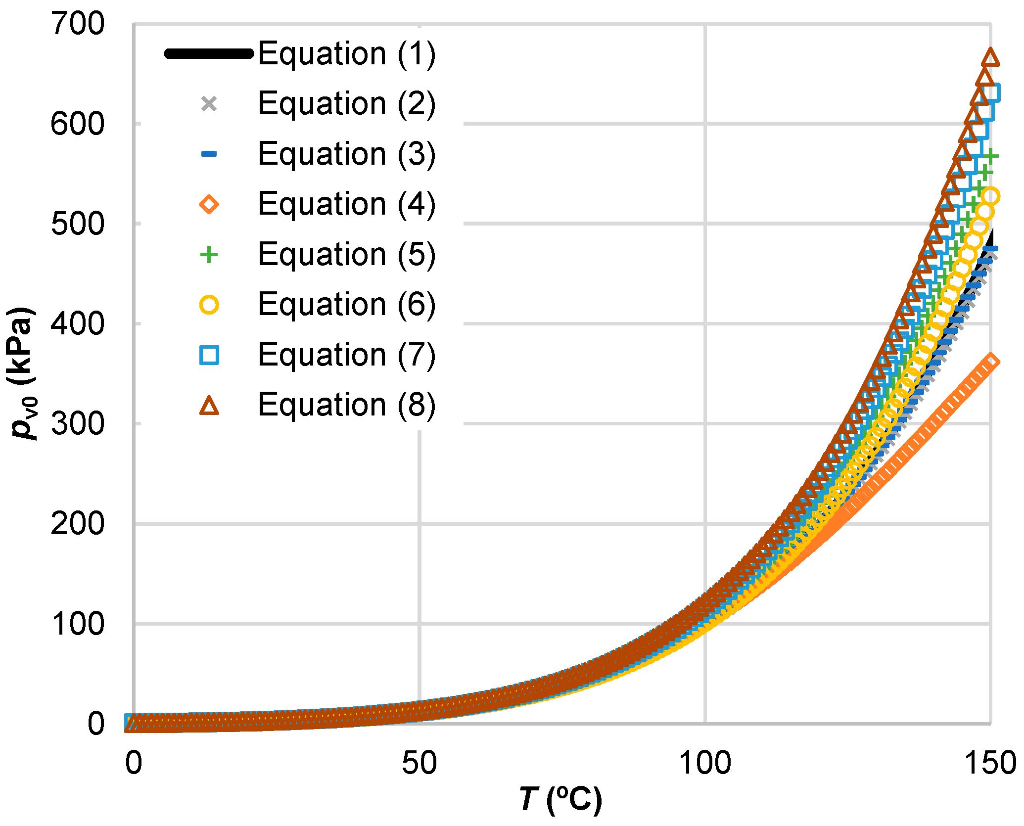
3.1. Saturated Water Vapour Pressure

The saturated water vapour pressure values obtained with the formulations in Table 1 are plotted as a function of temperature in Figure 1 for a temperature range between 0 and 150 °C.

Figure 1 shows that all the formulations inspected obtain similar values of the saturated water vapour pressure for the lower temperatures. However, the formulations diverge increasingly with temperature, with notable differences at 150 °C. To illustrate the drift of each formulation, their relative error RE_pv0, Equation (9), with respect to the reference of Equation (1) [4] is plotted in Figure 2.

Analysing Figure 2, Huang’s [6] equation, Equation (3), is the saturated water vapour pressure formulation with the least error in the temperature range analysed, 0–150 °C, and also in the more limited temperature range, 0–100 °C. The relative error of Equation (3) is kept within ±0.2% in the temperature range 0–150 °C, and is up to ±0.006% in the range 0–100 °C. Among the other formulations, only Buck’s [5] equation, Equation (2), limits its relative error under ±1.0% in the temperature range 0–150 °C. On the side of the lower accuracy, Equation (7), Nowak et al. [10] and Wang et al. [11], and Equation (8), Abed and Sołowski [12], both show relative errors higher than 10% for temperatures higher than 90 °C.

Equation (3) is able to reproduce the reference saturated water pressure values with a notably lower error than Equations (2) and (4)–(8). This result should not be surprising, since Equation (3) is the one containing the highest number of parameters from the equations in Table 1 after the reference of Wagner and Pruss [4], Equation (1), (5 compared to 2–4 parameters). Then, it should be analysed if the increase in number of parameters is justified or if, on the contrary, Equation (3) is overfitted. To this end, the AIC and the BIC were applied to the models, and the values of Akaike weights Aw from the AIC, Equation (11), and posterior model probabilities Bp from the BIC, Equation (13), were computed for all of them. For a number of observations equidistant between 0.01 and 150 °C of n = 3, Aw and Bp are plotted for Equations (2)−(8) in Figure 3. In the computations, the number of parameters k of Equations (2)−(8) are (4, 5, 3, 2, 2, 2, 2) (Table 1). The residual ε has been computed as the difference between the pressure obtained with each formulation and that of Equation (1). For any n, both information criteria for model selection yield the same result: the selected model for the data is Equation (3), the formulation by Huang [6]. It obtains Aw > 0.977 and Bp > 0.985 for any n ≥ 3, and Aw > 0.999 and Bp > 0.999 for any n ≥ 5. The rest of models, Equations (2) and (4)–(8), obtain Aw < 0.023 and Bp < 0.015 for any n ≥ 3, and tend to 0 with increasing n. Then, the increase in number of parameters for Equation (3) with respect to the rest of equations is justified with the increase in accuracy (information) they provide.

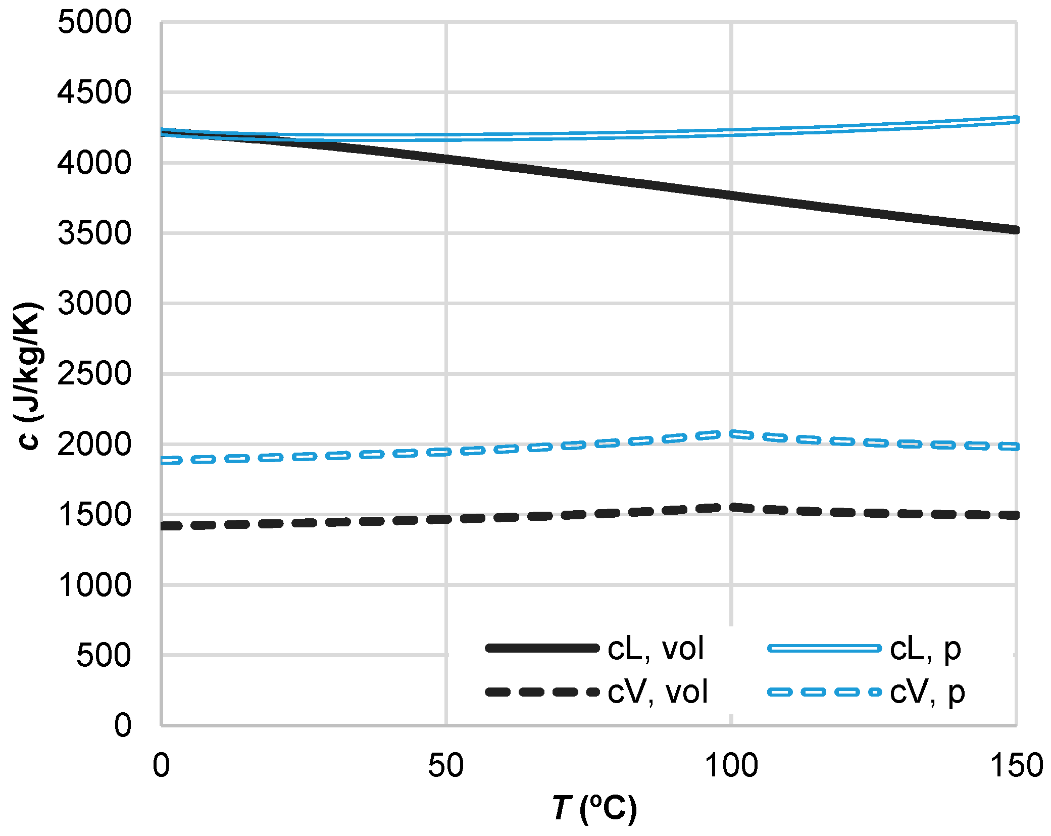
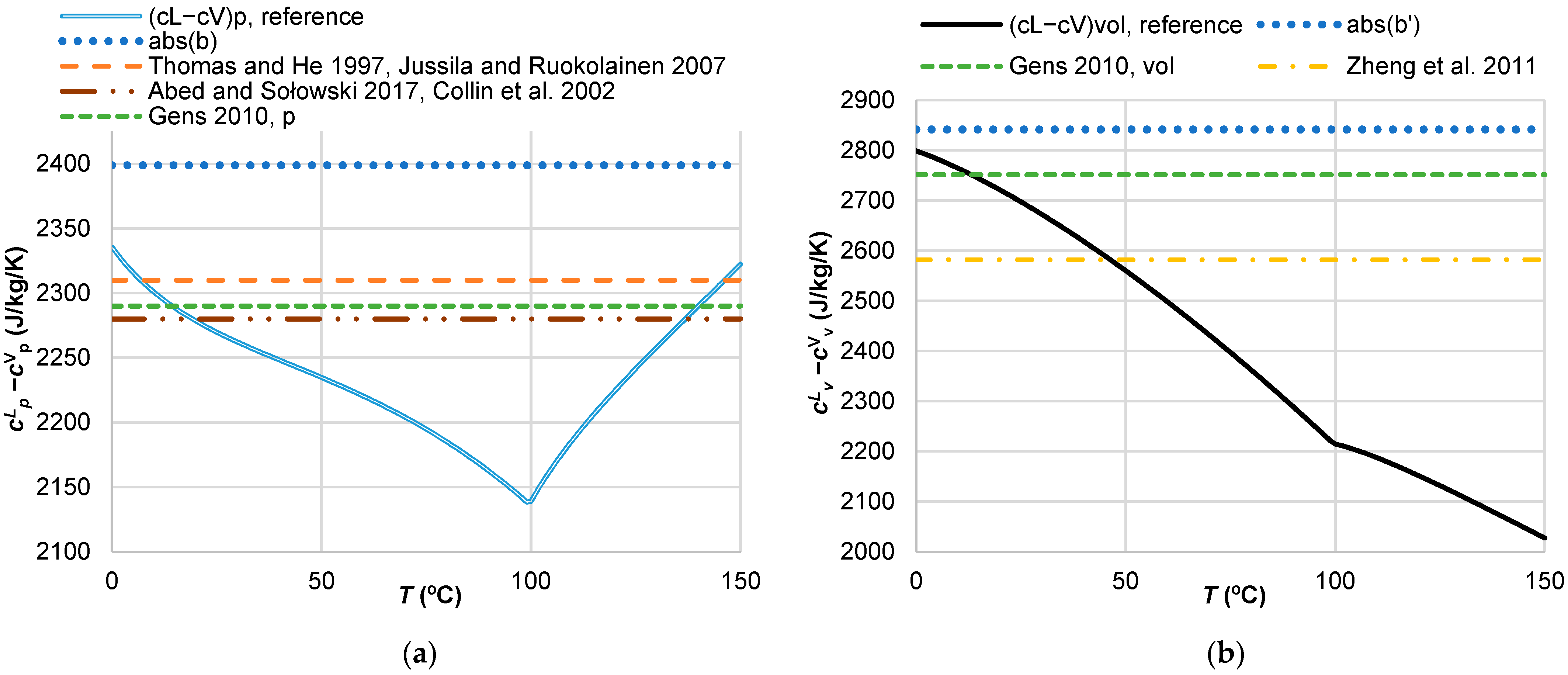
3.2. Vapour and Liquid Water Heat Capacities

Figure 4 plots the evolution of the reference enthalpy of vaporisation of water (Figure 4a) and the difference in internal energy between vapour and liquid water (Figure 4b) with temperature for the minimum pressure between saturated vapour pressure and 100 kPa. The source of the data is the NIST Chemistry WebBook [13]. The figure also plots the best linear fits Δh_LV = a + bT, Equation (23), and Δu_LV = a′ + b′T, Equation (25), to the data in the mentioned range, where the fitting parameters have been found to be a = 2500.9 kJ/kg, b = − 2.3989 kJ/kg/K, a′ = 2374.8 kJ/kg and b′ = − 2.8415 kJ/kg/K. The squared Pearson correlation coefficient R² obtained is nearly 1 for both Δh_LV and Δu_LV (Figure 4), which shows they are well represented with a linear fit. As mentioned, the difference in specific heat capacity between vapour and liquid water in isobaric conditions, c^V_p − c^L_p, Equation (22), should be close to the identified coefficient b, while the difference in isochoric conditions, c^V_v − c^L_v, Equation (24), should be close to the identified coefficient b′.

To illustrate the evolution of the specific heat capacities of liquid water and vapour with temperature, the values given by the NIST [13] for the range 0–150 °C are plotted in Figure 5. The figure includes values for isochoric and isobaric conditions at the minimum pressure between vapour saturation pressure and 100 kPa. Please note that, although the specific heat capacity of liquid water shows practically no dependence on pressure, that of water vapour does. For pressure conditions other than atmospheric, the corresponding specific heat capacity values can be obtained from the NIST [13], and an expression of the specific heat capacity of vapour as a function of pressure is found, for instance, in Vestfálová and Šafařík [24].

The temperature (and pressure) conditions corresponding to the specific heat capacity values used for modelling are not always reported in the literature. Then, a comparison of the literature and reference values is useful to identify such conditions and assess their consistency with the modelling conditions. The literature values in Table 2 are consistent with the reference values represented in Figure 5. The two values used for liquid water (4180 and 4202 J/kg/K) correspond to the reference specific heat capacities at 30 and 7 °C, respectively, for isobaric conditions, and at 13 and 6 °C, respectively, for isochoric conditions. The values used for water vapour in isobaric conditions (between 1870 and 1900 J/kg/K) correspond to the reference values between 0 and 15 °C. The vapour value specified for isochoric conditions (1428 J/kg/K) corresponds to the reference value at 11 °C. The vapour value given by Zheng et al. [17] (1620 J/kg/K) corresponds to the reference value in isochoric conditions at 121 °C although at saturation pressure. The vapour value given by Abed and Sołowski [12] (1900 J/kg/K) corresponds to the reference value in isobaric conditions at 15 °C.

However, the main interest in this study of the consistency of the formulation with the modelling of water vaporisation is the difference between the specific heat capacities of liquid water and vapour. The difference between the reference values in Figure 5 as a function of temperature from 0 to 150 °C is plotted in Figure 6, for both isobaric (Figure 6a) and isochoric (Figure 6b) conditions. In addition, the fit coefficients b and b’ identified from Figure 4 and the differences obtained from the literature values in Table 2, which are constant with temperature, are included for comparison.

Regarding the literature values (Table 2), all those given for isobaric conditions (Thomas and He [7], Collin et al. [14], Jussila and Ruokolainen [15] and Gens [16] (p)), or corresponding to such conditions according to the values in Figure 5 (Abed and Sołowski [12]), are consistent with the difference between isobaric reference values, since they are contained in the range of reference values for the studied temperatures (Figure 6a). The literature values for isochoric conditions (Gens [16] (vol), Zheng et al. [17]) are also consistent with the isochoric reference values (Figure 6b).

The absolute value of b, 2398.9 J/kg/K, is within a maximum relative error of 12% from the literature values and isobaric reference values. However, b is greater than reference values in all the temperature range (Figure 6a), which show a maximum of 2335.5 J/kg/K at 0 °C. Something similar occurs with the absolute value of b′, 2841.5 J/kg/K, which is greater than the maximum isochoric reference value, 2799.0 J/kg/K at 0 °C (Figure 6b). This result shows that using Equations (18)–(21) with a constant pair of specific heat capacities for liquid water and vapour equal to reference values at the same temperature (Figure 5), for any temperature between 0 and 150 °C, leads to underestimating the slope of the linear laws of Equations (22) and (24) plotted in Figure 4. Thus, it implies underestimating the decrease in Δh_LV or Δu_LV with temperature in the modelling. Assuming that the enthalpy of vaporisation, or the internal energy difference between vapour and liquid water, for the reference temperature, Δh_LV,T0 or Δu_LV,T0, is accurately set in the model, Δh_LV or Δu_LV will be accurately computed at T₀ and lose accuracy as temperature deviates from T₀.

To inspect this loss of accuracy, the evolution of Δh_LV and Δu_LV computed with Equations (22) and (24), respectively, in a case that would maximise this loss, has been studied and plotted in Figure 7. T₀ is set at one extreme of the temperature range considered, 0 °C, and Δh_LV,T0 and Δu_LV,T0 have been accurately taken as the reference values for 0 °C. Then, the maximum error will be made at the other extreme of the range, 150 °C, as a consequence of using a too small slope. To study the magnitude of the error at 150 °C, two values of the slopes (c^V_p − c^L_p) and (c^V_v − c^L_v) have been used. First, the values in the inspected literature furthest from the identified values for b and b′, from references [12,14] for Δh_LV (Figure 6a) and [17] for Δu_LV (Figure 6b), have been used (solid grey lines in Figure 7). In this case, the relative error at 150 °C is 0.7% for Δh_LV and 1.9% for Δu_LV. Second, the reference specific heat capacity pairs in Figure 6 furthest from b and b′ have been used: 2138 J/kg/K at 99 °C for isobaric values and 2027.3 J/kg/K at 150 °C for isochoric values (dashed orange lines in Figure 7). The relative error at 150 °C then increases to 1.7% for Δh_LV and 6.1% for Δu_LV.

Using the same approach, the relative error at 150 °C can, in addition, be computed for specific heat capacity pairs from the reference values [13] corresponding to all the temperature range between 0 and 150 °C (Figure 8). All errors are below the maximum errors mentioned in the previous paragraph (1.7% for Δh_LV and 6.1% for Δu_LV). If the relative error is to be further limited, the reference pairs used should be limited to lower temperatures. For instance, to limit the relative error to a 1%, for Δh_LV, any (c^V_p, c^L_p) pair from the literature values inspected would be valid, but the pairs of reference values for the same temperature should be limited to temperatures below 50 °C. Analogously, for Δu_LV, the pair of (c^V_v, c^L_v) from reference [16] would be valid, and the pairs of reference values for the same temperature should be limited to temperatures below 25 °C.

4. Conclusions

Two aspects relevant for a consistent thermo-hydraulic modelling of clay-based engineered barriers for deep geological repositories for radioactive waste have been studied: the saturated water vapour pressure and the specific heat capacity of liquid water and vapour. The temperature range of interest has been set between 0 and 150 °C.

Several expressions for the saturated water vapour pressure have been inspected, including reference expressions and those most applied in works modelling unsaturated soils and clay-based barriers. This has led to successfully identifying an accurate (relative error not greater than ±0.2%) and simple enough expression (ranked as the selected model using both the Akaike information criterion and the Bayesian information criterion), Huang’s [6] equation, Equation (3), as the optimal option for modelling in the temperature range between 0 and 150 °C.

Further, the enthalpy of vaporisation of water and the internal energy difference between liquid water and vapour as a function of temperature have been studied to derive the consistency of pairs of constant specific heat capacity values for liquid water and water vapour. Several pairs of values from the literature used for modelling unsaturated soils and clay-based barriers have been inspected. Their difference has been compared to reference values and to coefficients identified from the enthalpy of vaporisation and the difference of internal energy. It has been found that using constant specific heat capacity pairs corresponding to reference values at the same temperature can lead to underestimating the decrease in the enthalpy of vaporisation and of the internal energy difference with increasing temperature. To minimise this loss of accuracy, a model should use specific heat capacity pairs as close as possible to the fitted coefficient 2398.9 J/kg/K for isobaric values and 2841.5 J/kg/K for isochoric values. In the case of using reference specific heat capacity pairs for the same temperature, this means using pairs for a temperature as close to 0 °C as possible. However, the relative error associated with this loss of accuracy is limited, being below 2% for all the specific heat capacity pairs from the literature inspected, and up to a 6% for the reference specific heat capacity pairs for the same temperature between 0 and 150 °C.

References

1. Johnson, L.H.; Niemeyer, M.; Klubertanz, G.; Siegel, P.; Gribi, P. Calculations of the Temperature Evolution of a Repository for Spent Fuel, Vitrified High-Level Waste and Intermediate Level Waste in Opalinus Clay; Technical Report 01-04; Nagra: Wettingen, Switzerland, 2002. [Google Scholar]
2. Wagner, W.; Pruss, A. The IAPWS formulation 1995 for the thermodynamic properties of ordinary water substance for general and scientific use. J. Phys. Chem. Ref. Data 2002, 31, 387–535. [Google Scholar] [CrossRef] [Green Version]
3. Lemmon, E.W. Vapor pressure and other saturation properties of water. In CRC Handbook of Chemistry and Physics, 97th ed.; Haynes, W.M., Ed.; CRC Press: Boca Raton, FL, USA, 2017. [Google Scholar]
4. Wagner, W.; Pruss, A. International equations for the saturation properties of ordinary water substance—Revised according to the international temperature scale of 1990. J. Phys. Chem. Ref. Data 1993, 22, 783–787. [Google Scholar] [CrossRef] [Green Version]
5. Buck, A.L. New Equations for Computing Vapor Pressure and Enhancement Factor. J. Appl. Meteorol. Climatol. 1981, 20, 1527–1532. [Google Scholar] [CrossRef]
6. Huang, J. A Simple Accurate Formula for Calculating Saturation Vapor Pressure of Water and Ice. J. Appl. Meteorol. Climatol. 2018, 57, 1265–1272. [Google Scholar] [CrossRef]
7. Thomas, H.R.; He, Y. A coupled heat-moisture transfer theory for deformable unsaturated soil and its algorithmic implementation. Int. J. Numer. Methods Eng. 1997, 40, 3421–3441. [Google Scholar] [CrossRef]
8. Gens, A.; Sanchez, M.; Guimaraes, L.D.N.; Alonso, E.E.; Lloret, A.; Olivella, S.; Villar, M.V.; Huertas, F. A full-scale in situ heating test for high-level nuclear waste disposal: Observations, analysis and interpretation. Geotechnique 2009, 59, 377–399. [Google Scholar] [CrossRef]
9. Dupray, F.; François, B.; Laloui, L. Analysis of the FEBEX multi-barrier system including thermoplasticity of unsaturated bentonite. Int. J. Numer. Anal. Methods Geomech. 2013, 37, 399–422. [Google Scholar] [CrossRef]
10. Nowak, T.; Kunz, H.; Dixon, D.; Wang, W.; Görke, U.-J.; Kolditz, O. Coupled 3-D thermo-hydro-mechanical analysis of geotechnological in situ tests. Int. J. Rock Mech. Min. Sci. 2011, 48, 1–15. [Google Scholar] [CrossRef]
11. Wang, X.; Shao, H.; Wang, W.; Hesser, J.; Kolditz, O. Numerical modeling of heating and hydration experiments on bentonite pellets. Eng. Geol. 2015, 198, 94–106. [Google Scholar] [CrossRef]
12. Abed, A.A.; Sołowski, W.T. A study on how to couple thermo-hydro-mechanical behaviour of unsaturated soils: Physical equations, numerical implementation and examples. Comput. Geotech. 2017, 92, 132–155. [Google Scholar] [CrossRef]
13. Lemmon, E.W.; Bell, I.H.; Huber, M.L.; McLinden, M.O. Thermophysical Properties of Fluid Systems. In NIST Chemistry WebBook, NIST Standard Reference Database Number 69; Linstrom, P.J., Mallard, W.G., Eds.; National Institute of Standards and Technology: Gaithersburg, MD, USA, 2022. [Google Scholar] [CrossRef]
14. Collin, F.; Li, X.L.; Radu, J.P.; Charlier, R. Thermo-hydro-mechanical coupling in clay barriers. Eng. Geol. 2002, 64, 179–193. [Google Scholar] [CrossRef] [Green Version]
15. Jussila, P.; Ruokolainen, J. Thermomechanics of porous media—II: Thermo-hydro-mechanical model for compacted bentonite. Transp. Porous Media 2007, 67, 275–296. [Google Scholar] [CrossRef]
16. Gens, A. Soil-environment interactions in geotechnical engineering. Geotechnique 2010, 60, 3–74. [Google Scholar] [CrossRef]
17. Zheng, L.; Samper, J.; Montenegro, L. A coupled THC model of the FEBEX in situ test with bentonite swelling and chemical and thermal osmosis. J. Contam. Hydrol. 2011, 126, 45–60. [Google Scholar] [CrossRef] [PubMed] [Green Version]
18. Akaike, H. Information Theory as an Extension of the Maximum Likelihood Principle. In Second International Symposium on Information Theory; Petrov, B.N., Csaki, F., Eds.; Akademiai Kiado: Budapest, Hungary, 1973. [Google Scholar]
19. Schwarz, G. Estimating the Dimension of a Model. Ann. Stat. 1978, 6, 461–464. [Google Scholar] [CrossRef]
20. Çengel, Y.A.; Boles, M.A. Thermodynamics: An Engineering Approach; McGraw-Hill: New York, NY, USA, 1989. [Google Scholar]
21. Burnham, K.; Anderson, D.R. Multimodel Inference: Understanding AIC and BIC in Model Selection. Sociol. Methods Res. 2004, 33, 261–304. [Google Scholar] [CrossRef]
22. Pinder, G.F.; Shapiro, A. Physics of Flow in Geothermal Systems. Geol. Soc. Am. Spec. Pap. 1982, 189, 25–30. [Google Scholar] [CrossRef]
23. Navarro Gámir, V. Modelo del Comportamiento Mecánico e Hidráulico de Suelos No Saturados en Condiciones No Isotermas. Ph.D. Thesis, Universitat Politècnica de Catalunya, Barcelona, Spain, 1998. [Google Scholar]
24. Vestfálová, M.; Šafařík, P. Dependence of the isobaric specific heat capacity of water vapor on the pressure and temperature. EPJ Web Conf. 2016, 114, 02133. [Google Scholar] [CrossRef] [Green Version]
Figure 1. Saturated water vapour pressure as a function of temperature in the temperature range 0–150 °C for the different formulations analysed, Equations (1)–(8) [4,5,6,7,8,9,10,11,12]. Note that the results of Equations (2) and (3) practically overlap with the reference values of Equation (1).
Applsci 13 03361 g001
Figure 2. Relative error in the saturated water vapour pressure, REpv0, with respect to the reference, Equation (1) [4], as a function of temperature for the different formulations analysed. Equations (2)–(8) [5,6,7,8,9,10,11,12].
Applsci 13 03361 g002
Figure 3. Model selection results from information criteria for n = 3. Akaike weights Aw from the Akaike information criterion (blue), and posterior model probabilities Bp from the Bayesian information criterion (orange).
Applsci 13 03361 g003
Figure 4. (a) Enthalpy of vaporisation ΔhLV, and (b) difference in internal energy between vapour and liquid water ΔuLV, for temperatures between 0 and 150 °C. Markers: reference values from [13]. Line and equation: best linear fit.
Applsci 13 03361 g004
Figure 5. Specific heat capacity c of liquid (L, solid lines) water and water vapour (V, dashed lines) for the temperature range 0–150 °C, at the minimum between saturation pressure and 100 kPa, for isochoric (vol, black) and isobaric (p, blue outline) conditions. All values from the NIST [13].
Applsci 13 03361 g005
Figure 6. Difference in specific heat capacity between liquid water and vapour as a function of temperature. Solid lines: reference values [13] for (a) isobaric and (b) isochoric conditions; dotted and dashed lines: identified b and b′ coefficients and the literature values in Table 2 [7,12,14,15,16,17].
Applsci 13 03361 g006
Figure 7. Values of (a) ΔhLV and (b) ΔuLV computed with Equations (22) and (24), respectively, for specific heat capacity pairs that maximise error, from the literature (solid grey lines, values from [12,14], ΔhLV, and [17], ΔuLV) and from reference values (dashed orange lines). Reference ΔhLV and ΔuLV [13] in blue markers.
Applsci 13 03361 g007
Figure 8. Relative error in ΔhLV and ΔuLV at 150 °C using specific heat capacity pairs from reference values [13] at temperatures 0–150 °C.
Applsci 13 03361 g008