Multimodal Affective Communication Analysis: Fusing Speech Emotion and Text Sentiment Using Machine Learning

Abstract

Affective communication, encompassing verbal and non-verbal cues, is crucial for understanding human interactions. This study introduces a novel framework for enhancing emotional understanding by fusing speech emotion recognition (SER) and sentiment analysis (SA). We leverage diverse features and both classical and deep learning models, including Gaussian naive Bayes (GNB), support vector machines (SVMs), random forests (RFs), multilayer perceptron (MLP), and a 1D convolutional neural network (1D-CNN), to accurately discern and categorize emotions in speech. We further extract text sentiment from speech-to-text conversion, analyzing it using pre-trained models like bidirectional encoder representations from transformers (BERT), generative pre-trained transformer 2 (GPT-2), and logistic regression (LR). To improve individual model performance for both SER and SA, we employ an extended dynamic Bayesian mixture model (DBMM) ensemble classifier. Our most significant contribution is the development of a novel two-layered DBMM (2L-DBMM) for multimodal fusion. This model effectively integrates speech emotion and text sentiment, enabling the classification of more nuanced, second-level emotional states. Evaluating our framework on the EmoUERJ (Portuguese) and ESD (English) datasets, the extended DBMM achieves accuracy rates of 96% and 98% for SER, 85% and 95% for SA, and 96% and 98% for combined emotion classification using the 2L-DBMM, respectively. Our findings demonstrate the superior performance of the extended DBMM for individual modalities compared to individual classifiers and the 2L-DBMM for merging different modalities, highlighting the value of ensemble methods and multimodal fusion in affective communication analysis. The results underscore the potential of our approach in enhancing emotional understanding with broad applications in fields like mental health assessment, human–robot interaction, and cross-cultural communication.

1. Introduction

Affective communication, encompassing verbal and non-verbal cues, is essential for understanding and connecting with others on an emotional level. While facial expressions and other non-verbal modalities have successfully been used to detect emotions [1,2,3,4,5,6], speech is also a powerful channel for conveying emotional nuances. However, deciphering these emotions and sentiments embedded within speech remains a challenge, requiring advanced machine learning techniques. The implications of effectively recognizing emotional communication are far-reaching. In the domain of mental health, the ability to identify subtle emotional cues in speech holds promise for early detection and intervention of psychological distress [1,2,3,4]. Additionally, affective communication analysis can transform human–robot interaction applications, empowering AI systems to respond to human emotions more accurately and empathetically [5,6].

Beyond these domains, the insights gained from understanding affective communication can be applied to various fields, including healthcare, education, and customer service, where the ability to perceive and respond to human emotions is crucial.

This study investigates affective communication, exploring how the fusion of SER and SA can deepen our understanding of emotional dynamics in conversations. Recognizing the need for tools to identify and interpret emotions and sentiments in speech, we present a novel framework integrating both domains for a more comprehensive analysis.

Our primary objective is to create a framework that discerns and categorizes emotions and sentiments conveyed through speech. We utilize a hybrid methodology, employing traditional statistical features, deep learning techniques (1D-CNN), and classical machine learning algorithms (GNB, SVM, RF, MLP, and LR) to achieve this. Following the identification of the most effective individual classifiers for each dataset, we leverage our previously proposed dynamic Bayesian mixture model (DBMM) [2] for speech emotion recognition and sentiment analysis. This ensemble method, originally applied to activity recognition and facial expressions, is now adapted, and extended to the challenges of affective communication analysis. To further enhance our analysis, we incorporate sentiment derived from speech-to-text conversion, applying the same classification models to textual data. Our unique contribution lies in the integration of SER and SA through a novel two-layered dynamic Bayesian mixture model (2L-DBMM). This model, based on Bayesian inference, merges information from both domains, enabling the classification of more nuanced, second-level emotional states (Figure 1).

Thus, our main contributions are as follows:

• Novel Feature Engineering: Defining powerful hand-crafted features for speech emotion recognition (SER).
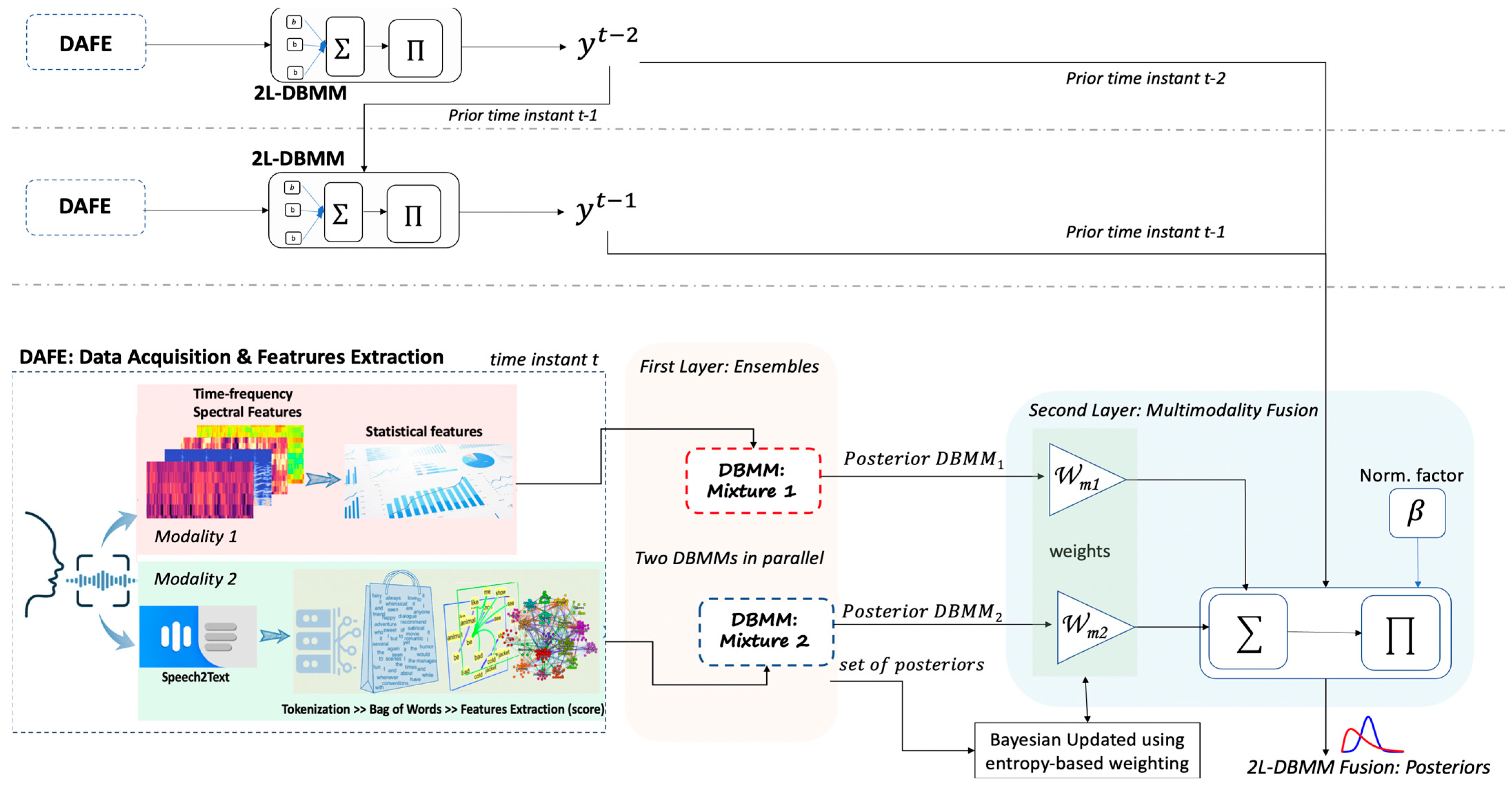
• Enhancement of DBMM: We adapt and extend the DBMM, previously demonstrated in [2,7], used for activity recognition, facial expressions, and semantic place categorization, to the domains of SER and SA. Our enhancement involves dynamically updating the classifier weights during test-set classification, rather than relying solely on pre-trained weights. This allows for the model to adapt to potential shifts in classifier performance over time. Furthermore, we employ a grid search optimization to determine the optimal number of time slices (previous priors) to incorporate in the model, enhancing the model’s ability to leverage temporal information and further improve classification accuracy.
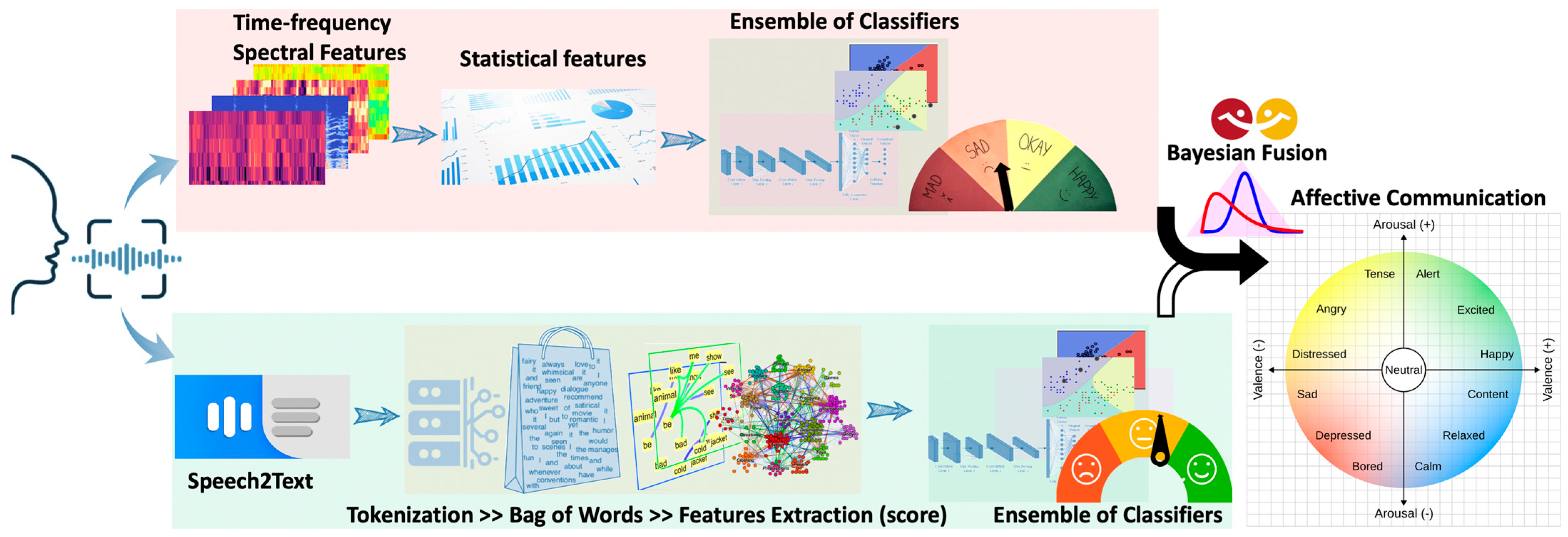
• Novel 2L-DBMM: Extending the DBMM to a two-layered model to enable multimodal fusion. This allows for not only the merging of individual classifiers for each modality, but also the fusion of multiple modalities (e.g., SER and SA) to achieve a more robust and nuanced understanding of affective communication. This novel 2L-DBMM model is the main contribution of this work, facilitating the recognition of new classes of emotional patterns derived from combined SER and SA data. This model can be generalized for fusion of diverse modalities.
• Extensive Validation and Insights: Conducting extensive tests and analysis on datasets to rigorously validate our proposed approach, providing comprehensive insights into the effectiveness and potential of our framework for real-world applications.

Our research has broad implications for various fields, including healthcare, human-robot interaction, and education. By providing a deeper understanding of affective communication, our framework has the potential to transform mental health diagnosis and treatment, personalize human–machine interactions with proper feedback, and foster more meaningful human connections in an increasingly digital world.

The structure of this paper is outlined as follows: Section 2 explores the background research reviewing the relevant literature. In Section 3, we introduce our proposed work and outline its development. Section 4 showcases our experimental results and insights. Finally, Section 5 presents the conclusions drawn from our findings and outlines avenues for future research.

2. Related Work

The fields of SER and SA have garnered significant attention due to their applications in diverse domains. This section outlines some key advancements and limitations in both areas, along with efforts towards their integration.

2.1. Speech Emotion

• Reviews and Trends: Lieskovská et al. [8] provide a comprehensive review of SER, highlighting the evolution of datasets, feature extraction techniques, and the increasing prominence of deep learning. While deep learning models have shown impressive performance, their limitations include the need for large, annotated datasets and high computational resources.
• INTERSPEECH 2019 Computational Paralinguistics Challenge: B. Schuller et al. [9] presented the outcomes of this challenge, which featured tasks related to SER, speaker traits, and emotion recognition in non-verbal vocalizations, fostering benchmarking and advances in paralinguistic analysis.
• Cross-Linguistic and Cross-Gender Challenges: Constantine et al. [10] investigate cross-linguistic and cross-gender SER, finding that while cross-linguistic tasks are achievable with high accuracy, cross-gender recognition is more challenging due to greater variability in emotional expression.
• Transfer Learning and Mel Spectrograms: Chakhtouna et al. [11] explore transfer learning for SER by converting Mel spectrograms into images and utilizing pre-trained models like VGG-16 and VGG-19. This approach demonstrates promising results, particularly when fine-tuning the models.
• Deep Learning for Emotion Detection: Zhao et al. [12] address the challenge of automatic emotion detection from speech, proposing a deep learning method combining knowledge transfer and self-attention for SER. Their self-attention transfer network (SATN) leverages attention autoencoders to transfer knowledge from speech recognition to SER, demonstrating effectiveness on the IEMOCAP dataset.
• Multi-task Learning: Latif et al. [13] propose a multi-task learning framework for SER, leveraging auxiliary tasks like gender identification and speaker recognition to enhance performance in scenarios with limited emotion datasets.
• Ensemble of Classifiers: Novais et al. [14] present a framework for speech emotion recognition that employs an ensemble of classifiers (RF and MLP) to enhance accuracy, achieving an 86% accuracy on the RAVDESS dataset.

2.2. Sentiment Analysis

• Social Media SA: Islam et al. [15] focus on sentiment analysis in social media, comparing lexicon-based and deep learning approaches. They find that deep learning models often outperform lexicon-based methods on social media platforms.
• Microblog Emotion Classification: Xu et al. [16] introduce the CNN_Text_Word2vec model for microblog emotion classification. By incorporating word2vec embeddings, they achieve higher accuracy compared to methods like SVM, LSTM, and RNN.
• Lifelong Learning: Lin et al. [17] propose lifelong text–audio sentiment analysis (LTASA) to enhance SA by incorporating audio modalities and enabling continuous learning of new tasks.
• Low-Resource Languages: Gladys and Vetriselvi [18] address the challenges of multimodal sentiment analysis (MSA) in low-resource languages like Tamil, leveraging cross-lingual transfer learning from larger English MSA datasets.

2.3. Multimodality Using SER and SA

• Multimodal Emotion Recognition: Kumar et al. [19] introduce VISTA-Net, a multimodal system classifying emotions using images, speech, and text inputs. They employ a hybrid fusion approach and achieve competitive accuracy on their IIT-R MMEmoRec dataset.
• Multimodal Sentiment Analysis from Videos: Poria et al. [20] develop a multimodal sentiment analysis framework emphasizing visual features’ importance and demonstrating significant novelty compared to existing works.
• Self-Supervised Learning: Atmaja and Sasou [21] investigate sentiment and emotion recognition from audio data using self-supervised learning with universal speech representations and speaker-aware pre-training models. Their results show promise, particularly in binary sentiment analysis tasks.

2.4. Current Challenges and Our Approach

Existing research in SER and SA still grapples with several challenges, including the need for large, annotated datasets, difficulties in cross-linguistic/gender recognition, and the need for more sophisticated fusion techniques. Additionally, model interpretability remains a concern. To address these limitations, our work introduces a novel approach to merging SER and SA through multimodal fusion, enabling a deeper understanding of affective communication. By combining speech signals with sentiment analysis from text, we aim to develop a framework that captures the emotional nuances of human communication, even across languages.

3. Proposed Approach

This section details our proposed approach, outlining the data processing steps and the classification model architectures utilized. Our research aims to create a more nuanced understanding of emotional expression by integrating SER and SA. This integration allows us to introduce a novel category of complex emotions, enriching the description of affective states within each utterance.

Table 1. Emotions from each modality and their combination.

SER	SA	Complex Emotion (Russell and Plutchik)	Theoretical Justification	Other References
Sad	Positive	Wistful, bittersweet, grieving	Low arousal (sad) + positive valence (positive sentiment) = mixed emotions, reflecting on positive past experiences with sadness due to their absence.	Mixed emotions are common and have been studied extensively [22].
Sad	Negative	Despair, hopelessness	Low arousal (sad) + negative valence (negative sentiment) = apathy and anhedonia, characteristic of depression.	The reinforcement of negative emotions is a hallmark of despair and possibly depression [23].
Sad	Neutral	Melancholy, pensive	Low arousal (sad) + neutral valence = sadness without strong positive or negative sentiment, associated with reflection.	Melancholy can be often associated with depression and other mood disorders [24].
Happy	Positive	Joyful, elated	High arousal (happy) + positive valence (positive sentiment) = intense happiness and excitement.	Positive emotions can be amplified through social contagion and emotional feedback loops [25].
Happy	Negative	Disingenuous, fake	Medium arousal (happy) + negative valence (negative sentiment) = masking true feelings with a facade of positivity.	Masking true feelings with a facade of happiness is a common defense mechanism [26].
Happy	Neutral	Content, serene	Medium arousal (happy) + neutral valence = calm and peaceful state of happiness.	This is a baseline state of positive affect without extreme intensity [27].
Neutral	Positive	Hopeful, optimistic	Low arousal (neutral) + positive valence (positive sentiment) = positive expectations for the future without intense emotion.	A neutral expression with positive sentiment may indicate optimism or resilience [28].
Neutral	Negative	Concerned, worried	Low arousal (neutral) + negative valence (negative sentiment) = negative expectations or outcomes without intense emotion.	These emotions are often associated with a lack of engagement or motivation [29].
Neutral	Neutral	Unsure, ambivalent	Low arousal (neutral) + neutral valence = uncertainty and lack of strong emotional inclination.	Uncertainty and ambivalence are common emotional states in decision-making or ambiguous situations [30].
Angry	Positive	Frustrated, irritated	High arousal (angry) + positive valence (positive sentiment) = anger combined with a desire for change or improvement.	Anger can be a powerful motivator for change and action [31].
Angry	Negative	Enraged, furious	High arousal (angry) + negative valence (negative sentiment) = uncontrolled anger and potential aggression.	Uncontrolled anger can lead to aggression and destructive behaviors [32].
Angry	Neutral	Annoyed, displeased	Medium arousal (angry) + negative valence (negative sentiment) = mild anger or irritation without intense rage.	Low-level anger can manifest as annoyance or frustration in response to minor obstacles [33].

presents the individual emotion classes for SER and SA, along with combined emotions used in our study to validate this approach.

When it comes to developing an approach for emotion recognition tasks, understanding the nuances of human emotion is paramount. Emotions are not always simple or discrete; they often manifest as complex blends of different affective states. To capture this complexity, we leverage Russell’s [34] arousal–valence model of affect and Plutchik’s wheel of emotions [35], two fundamental frameworks in the study of emotions in psychology that is relevant for affective computing. Russell’s model posits that emotions can be mapped onto a two-dimensional space defined by arousal (the intensity of the emotion) and valence (the pleasantness or unpleasantness of the emotion).

Plutchik’s wheel, on the other hand, categorizes emotions into primary (e.g., joy, sadness, anger, fear) and secondary (e.g., love, guilt, shame) categories, also considering their intensity.

In our study, we combine these frameworks to analyze complex emotions arising from the fusion of SER and SA. We consider speech emotion as a measure of arousal (angry, neutral, happy, sad, and surprise) and text sentiment as a measure of valence (positive, negative, and neutral). By mapping the different combinations of speech emotion and text sentiment onto the arousal–valence space, we can identify and label more nuanced emotional states.

For example, the combination of “sad” speech emotion (low arousal) and “positive” text sentiment (positive valence) might indicate a complex emotion like “wistful” or “bittersweet.” This reflects a state where the individual is experiencing sadness but also reminiscing about positive past experiences. Similarly, the combination of “angry” speech emotion (high arousal) and “positive” text sentiment might suggest “frustration” or “irritation,” indicating a desire for change or improvement despite the anger.

Table 1 presents a comprehensive overview of the complex emotions identified in our study, along with their theoretical justifications based on Russell’s [34] and Plutchik’s [35] models. By incorporating these psychological frameworks, we aim to provide a more nuanced and accurate representation of the emotional states captured by our multimodal fusion model. Primarily we follow Russell’s arousal–valence space, mapping emotions based on intensity and pleasantness. It also integrates elements from Plutchik’s wheel by considering primary emotions (e.g., happy, sad, angry) and their combinations to derive complex emotions. Specifically, the complex emotions can be seen as combinations of arousal and valence levels that derive complex emotions, like “joyful” (high arousal, positive valence) or “despair” (low arousal, negative valence). These are refined using Plutchik’s primary and secondary emotions to create nuanced labels (e.g., “wistful,” “frustrated”). Thus, Table 1 primarily follows Russell’s model but incorporates Plutchik’s categories for a more nuanced understanding of complex emotional states.

Figure 2 presents the frameworks for categorizing emotions, Russel’s [34] and Plutchik’s [35] models.

3.1. Speech Features Extraction

In the domain of SER, the process of feature extraction holds a crucial role in capturing pertinent information from speech signals. This section presents our approach to feature engineering from audio recordings for emotion recognition tasks.

The selection of specific features (Algorithm 1) such as Mel frequency cepstral coefficients (MFCCs), Mel spectrogram, Chroma, and Tonnetz is substantiated by their capability to capture distinct aspects of the audio signal, thereby enhancing the efficacy of subsequent emotion recognition tasks. The relevance of using these features is underscored by their unique contributions. MFCCs are widely employed in speech processing, since they encapsulate the short-term power spectrum of a sound, offering insights into its spectral characteristics. Mel Spectrogram representation offers valuable insights into the distribution of energy across different frequency bands in the Mel frequency scale, enriching our understanding of spectral dynamics. Chroma features captures the distribution of energy across the 12 pitch classes of the musical octave, providing crucial information about the harmonic content and tonal structure of the audio signal. Tonnetz features extracted from the harmonic component of the audio signal (tonal space), offer valuable insights into the tonal centroid, aiding in the characterization of harmonic relationships.

After extracting time–frequency spectrogram-based features, the computation of statistical features derived from these outputs serves to reduce dimensionality while preserving significant information from the time–frequency spectrograms. These statistical features, represented by mean, standard deviation, and moments effectively summarize the distribution and characteristics of the audio signal.

Additional features such as Pitch, Energy, Zero Crossing Rate, and RMS Energy are employed because they capture pitch-related, amplitude-related, and temporal characteristics, offering a comprehensive understanding of the speech signal’s dynamics.

By leveraging these diverse features, we construct a feature vector that encapsulates both spectral and temporal aspects of the audio signal. Subsequent normalization ensures that these features are uniformly scaled, facilitating the convergence and performance of machine learning algorithms in emotion recognition tasks. This approach of extracting statistical information from time–frequency spectrogram-based features yields an efficient and informative representation of the audio signal, conducive to accurate emotion classification.

Algorithm 1. SER: Features Extraction

3.2. Sentiment Analysis Feature Extraction

In the domain of sentiment analysis, the process of feature extraction plays a pivotal role in deriving meaningful representations from text inputs, subsequently utilized for sentiment classification tasks. This subsection presents our chosen feature engineering, drawing from established techniques in the literature. The preprocessing pipeline begins with the conversion of audio inputs to text using speech-to-text techniques (e.g., API such as Google Cloud Speech-to-Text since it covers a range of languages). Once the audio is transcribed into textual form, further preprocessing steps are employed to prepare the text data for feature extraction. Tokenization is applied to segment the text into individual tokens, typically words or subword units.

The process of tokenization facilitates the creation of a bag-of-words (BoW) representation, where the frequency of occurrence of each token in the text corpus is recorded. BoW encoding captures the presence or absence of words in the text, disregarding their order, and serves as the basis for subsequent feature extraction. Feature extraction techniques based on scores are then utilized to derive sentiment-specific features from the BoW representation. These features include sentiment lexicons, word embeddings, and statistical measures computed from the BoW vectors. In this study we focus on the frequency–inverse document frequency (TF-IDF) weighting scheme, which is used to quantify the importance of terms in a document relative to a corpus.

TF-IDF consists of two components: (i) Term frequency (TF) measures how frequently a term appears in a document. TF is calculated by dividing the number of times a term occurs in a document by the total number of terms in the document. (ii) Inverse document frequency (IDF) measures the rarity of a term across all documents in the corpus. It is calculated by dividing the total number of documents by the number of documents containing the term, and then taking the logarithm of that quotient. The TF-IDF score for a term in a document is obtained by multiplying its TF and IDF values. Higher TF-IDF scores indicate terms that are more important or relevant to the document. Algorithm 2 presents the step by step for the SA features extraction.

Algorithm 2. SA: Features Extraction

Input: Text data from audio signal (speech2text)

Result: Feature vector for sentiment analysis classification

1. Pre-processing:

a. Tokenization:

-Tokenize the text data into individual words or tokens.

b. Text Cleaning:

-Remove punctuation, special characters, and irrelevant symbols.

-Convert all text to lowercase for consistency.

2. Bag of Words Representation:

-Represent the text data as a bag of words by counting the frequency of each word in the corpus.

3. Feature Extraction:

a. Term Frequency (TF):

-Compute the TF score for each term in each document.

-TF(t, d) = (Number of times term t appears in document d) / (Total number of terms in doc d)

b. Inverse Document Frequency (IDF):

-Compute the IDF score for each term across the entire corpus.

-IDF(t) = log_e(Total of documents / Number of documents containing term t)

c. TF-IDF Score:

-Calculate the TF-IDF score for each term in each document.

-TF-IDF(t, d) = TF(t, d) × IDF(t)

4. Feature Vector Construction:

-Concatenate the TF-IDF scores for all terms in each document into a vector.

-Each document is represented as a vector of TF-IDF scores, where each dimension corresponds to a unique term in the vocabulary.

Output: Feature vector representing the features for Sentiment classification.

3.3. DBMM as Ensemble for Single Modality and 2L-DBMM for Multimodality

We employ a probabilistic framework to enhance the recognition of affective communication by leveraging the complementary strengths of multiple classifiers for speech emotion and sentiment analysis, extracted from both audio and text data. We utilize the DBMM, a flexible and dynamic probabilistic framework previously showcased in our work [7]. The DBMM is an ensemble of classifiers that merges conditional probability outputs from different base classifiers to enhance overall performance. Each classifier is assigned a weight based on prior knowledge and an uncertainty measure, such as confidence levels, acquired during training. This allows for the model to dynamically update classifier weights at runtime, accounting for potential variations in individual classifier performance. The DBMM also incorporates prior information to iteratively reinforce current classifications. In this study, we further enhance the DBMM with dynamic weight updates during classification, based on historical behaviors of the base classifiers. Additionally, we implement a grid-based optimization to search for the optimal number of time slices for the DBMM, determining the extent of temporal information to incorporate as new priors. The general model of DBMM is given by computing the posterior distribution P(C|A) at time instant t as follows:

$$P\left(C^t|C^{t-1:t-T},A^t\right)={\displaystyle \frac{{\prod }_{k=t}^{t-T}P\left(C^k|C^{k-1}\right)\times {\sum }_{i=1}^N{w}_i^t\times P_i\left(A^t|C^t\right)}{{\sum }_{j=1}^{classes}\left[{\prod }_{k=t}^{t-T}{P}_{i,j} \left(C^k|C^{k-1}\right)\times {\sum }_{i=1}^N{w}_i^t\times P_{i,j}\left(A^t|C^t\right)\right]}},$$

(1)

where P(C^k|C^k−1) is the prior information (previous ensemble posteriors), and w_i^t is the weight for each ith base classifier, which was learned previously using any uncertainty measure applied to a dataset or to a temporal window with previous predictions from the base classifiers. P_i (A^t│C^t) is the likelihood resulted given the posterior of each base classifier.

An alternative to attain w_i for each base classifier based on their confidence is computing the inverse entropy to update the global probabilistic model.

Weights are computed by analyzing base classifiers previous outputs (i.e., learned form a dataset or from previous time instants). We can compute the inverse entropy of the posterior probabilities previously observed as follows:

$$w_i=1-\left({\displaystyle \frac{-{\sum }_{k=1}^s{P}_{i,k}\left(·\right)\log \left(P_{i,k}\left(·\right)\right)}{{\sum }_{i=1}^N\left(-{\sum }_{k=1}^s{P}_{i,k}\left(·\right)\log \left(P_{i,k}\left(·\right)\right)\right)}}\right),$$

(2)

where P_i,k(·) = P_i,k(C|A) is the class conditional probability given the model of an ith base classifier and s is the number of posteriors used.

During classification tasks, individual models within an ensemble may exhibit varying performance over time. To address this and improve overall classification accuracy, we employ a strategy of locally updating weights during classification. This approach identifies classifiers showing increased fluctuations in performance (e.g., frequent accuracy drops) and reduces their confidence accordingly. We adjust weights based on past performances of base classifiers on observed frames, assigning higher weights to those with better performance. Assuming the system’s memory follows the Markov property during online classification, we utilize temporal information from the set of posteriors for each classifier: $P\left(C_i^t|C_i^{t-1}\right);\mathrm{ }P\left(C_i^{t-1}|C_i^{t-2}\right); P\left(C_i^{t-2}|C_i^{t-3}\right) \dots P\left(C_i^{t-s}|C_i^{t-\left(s-1\right)}\right).$

This temporal information is integrated into the Bayesian update model to compute likelihood by recalculating entropy h, coupled with weights from the previous time instant w_i^(t−1) as prior knowledge. The resulting updated probability serves as new weights for each base classifier in the current frame classification.

The Bayesian update is expressed as follows:

$$w_i^t=P\left(w_i|h_i\right)={\displaystyle \frac{P\left(h_i|w_i\right)P\left(w_i\right)}{{\sum }_{i=1}^{N}P\left(h_i|w_i\right)P\left(w_i\right)}},$$

(3)

where P(h_i|w_i) is given by (2) for each ith base classifier using their previous frames posteriors and the prior P(w_i) = w_i^t−1.

While the DBMM effectively combines multiple classifiers within a single modality, our novel contribution lies in extending it to a two-layered model (2L-DBMM) for multimodal fusion. The 2L-DBMM consists of two separate DBMMs, one for SER another for SA.

Each DBMM operates independently on its respective modality, combining the outputs of multiple base classifiers. The final step involves a fusion layer that merges the outputs of the two DBMMs, creating a new class of emotion that combines both speech emotion and text sentiment. This approach allows for a more nuanced and comprehensive understanding of affective communication by leveraging the strengths of both modalities.

This two-layered architecture (Figure 3) not only captures the complementary strengths of multiple classifiers within each modality but also allows for a more robust and nuanced understanding of affective communication by considering the interplay between speech emotion and text sentiment.

Then proposed 2L-DBMM is computed as follows:

$$P\left(C^t|A^t\right)={\displaystyle \frac{1}{\beta }}\times \prod _{k=t}^{t-T}\left\{\stackrel{\mathrm{dynamic} \mathrm{prior}}{\overbrace{ P\left(C^k\right|C^{k-1})}} \times \stackrel{\mathrm{fusion} \mathrm{of} \mathrm{multiple} \mathrm{mixtures}=\mathrm{modalities}}{\overbrace{ \sum _{y=1}^M\left[w_{2_y}^k\times \left(\underset{\mathrm{fusion} \mathrm{of} \mathrm{base} \mathrm{classifiers}}{\underbrace{\sum _{i=1}^N{w}_{1_{y,i}}^k\hspace{0.17em}\hspace{0.17em}{P}_{y,i}\left(A^k|C^k\right)}}\right)\right]}}\right\},$$

(4)

where P(C^t|A^t) is the resulting posterior; C represents classes of emotions; A represents the set of feature models; 1/β is a normalization factor; the dynamic prior P(C^k|C^k−1) is obtained from the set of posteriors from previous time slices; y = {1, …, M} is an index to represent the mixture models = number of modalities; i = {1, …, N} is an index to represent the base classifiers; t is the current time instant, k is an index to represent the time instants, and T is the number of time slices used in the model (i.e., number of previous posteriors used as prior to reinforce the current classification); P(A|C) denotes the output conditional probability from a learning model (i.e., base classifier); w₁ is the first layer’s weight used for fusion; and w₂ is the second layer’s weight to merge all modalities, in this study, two. In this model, the weights w_y can be computed through any uncertainty measure (e.g., entropy-based).

It is important to highlight that the 2L-DBMM introduces a fundamental shift in how dynamic weights are updated within the ensemble learning framework. By incorporating a dynamic weighting mechanism based on the temporal evolution of classifier performance, the 2L-DBMM captures the varying reliability of different modalities over time, leading to a more adaptive and robust fusion strategy. Initially, the model receives handcrafted features based on spectral feature statistics, which feed two modified DBMM models. These models utilize uncertainty measures to assess the confidence of each inference model, both during training and real-time classification. This on-the-fly classification is enhanced by using inverse entropy-based weighting and Bayesian updates of the weights over time. This approach incorporates learned weights as priors, updating them based on the inverse entropy of the current classification, allowing for the model to adapt to changes in classifier behavior. Our research demonstrates that updating the weights in each modality (classifiers to build the ensemble) can lead to a 3% improvement in final accuracy compared to using static weights from the training set. This strategy is then applied to the second layer, where the uncertainty of each modality is measured during training, and Bayesian updates during the test set further optimize the fusion model’s accuracy. Additionally, incorporating temporal information, such as previous time slices (posterior probabilities), reinforces overall classification performance. Furthermore, the inclusion of grid search optimization to determine the optimal number of time slices for incorporating past information enhances the model’s flexibility and performance. This optimization enables the model to tailor its fusion strategy to the data’s specific characteristics. Techniques such as measuring uncertainties of individual classifiers, assessing uncertainties of each modality, updating them over time based on classifier and modality behavior, and determining the optimal number of time slices for the data fusion step are all employed to improve the model.

3.4. Classical Machine Learning Models for DBMM

3.4.1. DBMM’s Base Classifier Configurations and Parameters for SER

We utilized several well-known classical machine learning models as base classifiers in this research: SVM, GNB, RF, 1D-CNN, and MLP. The specific configurations and parameters used for each model are outlined in

Table 2. Classifier parameters for SER.

Classifier	Configuration/Parameters	Notes
SVM	Linear kernel Regularization parameter (C) = 1.0	A linear kernel is often effective for high-dimensional feature spaces in SER tasks.
RF	150 decision trees	The number of trees is a hyperparameter tuned for optimal performance.
GNB	Gaussian distribution	Assumes that features are conditionally independent given the class, which is a simplification but often works in practice for SER.
MLP	3 dense layers with ReLU activation 320 neurons in layer 1 192 neurons in layer 2 Softmax activation in the output layer 350 epochs, batch size = 256	ReLU activation is used for non-linearity, and softmax for multi-class probability distribution. Epochs and batch size are hyperparameters controlling training duration and update frequency.
1D-CNN	1 convolutional layer 128 filters, kernel size = 3 Max-pooling layer (size = 2) Flattened output into dense layer with softmax activation 350 epochs, batch size = 32	Convolutional layers capture local patterns, max-pooling reduces dimensionality, and the dense layer with softmax outputs class probabilities.
DBMM	3 classifiers: 1D-CNN, MLP, RF 2 time slices (previous priors) Entropy-based weights Bayesian update of weights	Initial weights are based on performance on the training set and are dynamically updated during test-set classification. A grid search optimization is employed to find the optimal number of time slices (past predictions) to incorporate as prior information.

.

• SVM: A supervised learning algorithm that seeks to find the optimal hyperplane that maximally separates different classes in a high-dimensional feature space. In our implementation, we employ a linear kernel due to its computational efficiency and effectiveness for our specific feature set. The regularization parameter (C), a hyperparameter controlling the trade-off between maximizing the margin and minimizing classification error, is set to 1.0.
• RF: An ensemble learning method that constructs multiple decision trees during training. The final prediction is determined by aggregating the predictions of individual trees, typically by taking the mode of the classes (for classification) or the mean prediction (for regression). We utilize 150 decision trees in our RF model, a parameter chosen through empirical experimentation.
• GNB: A simple probabilistic classifier based on Bayes’ theorem with the “naive” assumption of feature independence. Despite this simplifying assumption, GNB often performs surprisingly well in practice, especially when the features are not strongly correlated.
• MLP: A class of feedforward artificial neural network composed of multiple layers of interconnected nodes. Our MLP model comprises three dense (fully connected) layers. The hidden layers utilize rectified linear unit (ReLU) activation functions, introducing non-linearity to model complex relationships. The output layer employs a softmax activation function to produce probability distributions over the multiple emotion classes.
• The 1D-CNN is trained for 350 epochs with a batch size of 256. The first hidden layer contains 320 neurons, while the second has 192. The output layer consists of a number of neurons equal to the number of target classes.

3.4.2. Base Classifiers for Sentiment Analysis

For sentiment analysis, we employed both pre-trained language models and classical machine learning algorithms, with specific configurations and parameters for each, as detailed in

Table 3. Classifier parameters for SA.

Classifier	Configuration/Parameters	Notes
BERT	Fine-tuned for sequence classification 3 labels AdamW optimizer Cross-entropy loss 350 epochs, batch size = 32 Linear learning rate scheduler with warmup	Transformer-based model for natural language processing.
GPT-2	Fine-tuned for sequence classification 3 labels AdamW optimizer Cross-entropy loss 350 epochs, batch size = 32 Linear learning rate scheduler with warmup	Transformer-based model for text generation.
LR	Default parameters, max iterations = 1500, TF-IDF features	Simple and interpretable linear model.
SVM	Linear kernel, C = 1.0, TF-IDF features	Effective for high-dimensional text data.
RF	100 decision trees, TF-IDF features	Ensemble method combining multiple decision trees.
MLP	2 hidden layers (320, 192 neurons) Adam optimizer TF-IDF features	Neural network for non-linear modeling.
1D-CNN	1 convolutional layer 128 filters, kernel size = 3 Max-pooling layer (pooling size = 2), Flattened output into dense layer with softmax activation, 350 epochs, batch size = 32	Adapted for sequential text input.
DBMM	3 Classifiers: BERT, SVM, RF 2 time-slices (previous priors) Entropy-based weights Bayesian update of weights	A grid search optimization is employed to find the optimal number of time slices (past predictions) to incorporate as prior information.

and explained below:

• BERT (BERT base uncased): This model leverages a transformer architecture with self-attention mechanisms to capture contextual relationships in text. We fine-tuned it for sequence classification using pre-trained weights and optimized it with the AdamW optimizer (with weight decay) and cross-entropy loss over 350 epochs, using a batch size of 32 and a linear learning rate scheduler with warmup steps.
• GPT-2: Similarly, this transformer-based model was fine-tuned for sequence classification with the same configuration as BERT. However, its architecture relies on decoder blocks, specialized for sequential text generation.
• Logistic regression: We applied this simple linear model with default parameters (maximum iterations = 1500) to TF-IDF features extracted from text data.
• SVM: This model, effective for high-dimensional text data, was configured with a linear kernel and a regularization parameter (C) of 1.0 to control overfitting. It was trained on TF-IDF features.
• RF: This ensemble method combines the predictions of multiple decision trees for improved accuracy. Our RF model utilized 100 decision trees and was trained on TF-IDF features.
• MLP: Designed with two hidden layers (320 and 192 neurons), was trained on TF-IDF features using the Adam optimizer. ReLU activation was used in the hidden layers, and a softmax activation function was employed in the output layer for multi-class classification.
• 1D-CNN: We adapted the architecture from our SER experiments to the sentiment analysis task. This model, composed of convolutional, max-pooling, and dense layers, was trained on reshaped text data for sequential analysis.

4. Results

4.1. Speech Emotion Datasets and Experimental Setup

In this work, our approach was evaluated using two distinct datasets, each offering unique characteristics for assessing affective communication analysis across different languages and emotional expressions.

The EmoUERJ dataset [36] consists of 377 audio recordings in Portuguese, encompassing four distinct emotional categories: happiness, anger, sadness, and neutral. These recordings were obtained from eight actors, evenly split between male and female, who each contributed ten sentences selected from a set of daily routine phrases. This dataset provides a valuable resource for understanding emotional expression within a specific cultural and linguistic context.

On the other hand, the Emotional Speech Dataset (ESD) [37] is a multilingual dataset comprising 350 parallel utterances across five emotions: anger, sadness, surprise, neutral, and happiness. Recorded by 10 native English and 10 native Chinese speakers, with equal representation of genders, this dataset allows for a comparative analysis of emotional expression across different languages. For this study, we focused solely on the English portion of the ESD.

To assess the performance of our models in a more comprehensive manner, we combined the EmoUERJ (Portuguese) and ESD (English) datasets into a multilingual dataset. This cross-linguistic approach allowed for us to evaluate how effectively our framework captures emotional patterns across different languages and cultures. To train and validate our classifiers, we employed a standard 80/20 split strategy (train/test) for both individual and combined datasets.

Our experimental setup utilized a MacBook Pro M1 Max, equipped with a 10-core CPU (8 performance cores and 2 efficiency cores), a 32-core GPU, and 64 GB of unified memory. This configuration provided efficient parallel processing capabilities, accelerating training and inference for our machine learning models. The EmoUERJ and ESD datasets were both trained and tested on this setup, utilizing the hardware acceleration for optimal performance.

4.2. Validation of the Proposed Approach on the EmoUERJ Dataset

The overall performance achieved using the designed audio features and five in-dividual classifiers (1D-CNN, SVM, RF, GNB, and MLP) on the EmoUERJ dataset is presented in

Table 4. Overall performance using multiple classifiers on EmoUERJ dataset.

Classifier	Overall PREC	Overall REC	Overall F1-Score	Overall ACC
1D-CNN	0.89	0.84	0.84	0.86
SVM	0.75	0.76	0.74	0.73
RF	0.78	0.79	0.77	0.76
GNB	0.73	0.75	0.73	0.72
MLP	0.79	0.81	0.79	0.77
DBMM	0.95	0.93	0.94	0.94

, along with the ensemble model DBMM.

Table 5. Classification results per emotion on EmoUERJ dataset.

(a) 1D CNN					(b) SVM
	PREC	REC	F1	Support		PREC	REC	F1	Support
Happy	0.89	0.7	0.78	26	Happy	0.79	0.59	0.67	26
Neutral	0.95	0.79	0.86	17	Neutral	0.72	0.64	0.67	17
Sad	0.95	0.96	0.95	14	Sad	0.85	0.91	0.88	14
Angry	0.78	0.92	0.85	19	Angry	0.64	0.89	0.75	19
ACC			0.86	76	ACC			0.73	76
Macro avg	0.89	0.84	0.86	76	Macro avg	0.75	0.76	0.73	76
Weighted avg	0.89	0.84	0.84	76	Weight avg	0.75	0.73	0.73	76
(c) RF					(d) GNB
	PREC	REC	F1	Support		PREC	REC	F1	Support
Happy	0.87	0.59	0.7	26	Happy	0.77	0.66	0.71	26
Neutral	0.81	0.81	0.81	17	Neutral	0.81	0.63	0.71	17
Sad	0.8	0.91	0.85	14	Sad	0.71	1	0.84	14
Angry	0.63	0.84	0.72	19	Angry	0.64	0.67	0.66	19
ACC			0.76	76	ACC			0.72	76
Macro avg	0.78	0.79	0.77	76	Macro avg	0.74	0.75	0.73	76
Weight avg	0.79	0.76	0.81	76	Weight avg	0.74	0.72	0.72	76
(e) MLP					(f) DBMM
	PREC	REC	F1	Support		PREC	REC	F1	Support
Happy	0.75	0.59	0.66	26	Happy	0.95	0.89	0.92	26
Neutral	0.83	0.87	0.85	17	Neutral	0.99	0.96	0.98	17
Sad	0.92	0.98	0.95	14	Sad	0.96	0.97	0.97	14
Angry	0.66	0.79	0.72	19	Angry	0.88	0.91	0.90	19
ACC			0.77	76	ACC			0.94	76
Macro avg	0.79	0.81	0.79	76	Macro avg	0.95	0.93	0.94	76
Weight avg	0.78	0.77	0.77	76	Weight avg	0.95	0.93	0.94	76

details the performance of each classifier per emotion within the same dataset.

Table 6. Comparative analysis of our approach with the study referenced in [38].

Method	Training Language	Tested Language	ACC
Wav2Vec2-XLSR [25]	Portuguese (EmoUERJ)	Portuguese (EmoUERJ)	0.92
Wav2Vec2-XLSR [25]	English (ESD)	Portuguese (EmoUERJ)	0.88
Our Approach	Portuguese (EmoUERJ)	Portuguese (EmoUERJ)	0.94
Our Approach	English (ESD)	Portuguese (EmoUERJ)	0.94

presents a comparative analysis of our approach and the study presented in [38] for the EmoUERJ dataset.

• Individual Classifier Performance: The 1D-CNN model consistently outperformed other individual classifiers across most emotions. It achieved the highest accuracy for “happy” (89%) and “sad” (95%) emotions. However, its performance was slightly lower for “neutral” (79%) and “angry” (78%) emotions. The RF model demonstrated comparable performance to 1D-CNN for “sad” (91%) and “angry” (84%) emotions. However, it exhibited lower accuracy for “happy” (59%) and “neutral” (81%) emotions. GNB performed moderately well on “happy” (77%) and “neutral” (81%) emotions but showed lower accuracy for “sad” (71%) and “angry” (64%) emotions. The MLP model performed well across all emotions, with high accuracy for “sad” (95%) and “angry” (79%). Its performance for “happy” (75%) and “neutral” (87%) was competitive with other classifiers. Analyzing the overall results, the top three individual classifiers are 1D-CNN, MLP, and RF.
• Ensemble Model Performance (DBMM): The DBMM ensemble model, combining the 1D-CNN, MLP, and RF classifiers, significantly outperformed all individual classifiers on the EmoUERJ dataset. It achieved the highest overall accuracy of 94%, with precision, recall, and F1-score all at 94%. This demonstrates the effectiveness of ensemble methods in leveraging the strengths of different classifiers to improve overall performance. The DBMM excelled in classifying the “neutral” emotion (99% precision, 96% recall, 98% F1-score), which was a challenge for some individual classifiers.
• Cross-Linguistic Analysis: The results in Table 6 compare the performance of our feature model + DBMM when trained on the EmoUERJ dataset and tested on both EmoUERJ and the ESD (English) dataset. Our model demonstrated high competitiveness with the study presented by [38] when tested on EmoUERJ. While our approach achieved high performance when trained on the ESD dataset and tested on the EmoUERJ dataset, the opposite scenario, training on EmoUERJ and testing on ESD, resulted in lower performance. This suggests that the model trained on the Portuguese EmoUERJ dataset might not generalize well to the English language dataset, likely due to differences in acoustic features and emotional expression patterns between languages.
• Discussion: The results on the EmoUERJ dataset underscore the effectiveness of ensemble-based methods like DBMM in improving speech emotion recognition performance compared to individual classifiers. Among the individual classifiers, 1D-CNN emerged as the strongest performer, closely followed by MLP. These findings suggest that deep learning models, when combined with appropriate feature engineering, can effectively capture and classify emotional nuances in speech. The cross-linguistic analysis emphasizes the need for further exploration of models and techniques that can generalize well across different languages and cultural contexts. Future work could explore methods for adapting models to different languages or creating more language-agnostic features.

4.3. Validation of the Proposed Approach on the Emotional Speech Dataset (ESD)

We evaluated the performance of five individual classifiers (1D-CNN, SVM, RF, GNB, and MLP) and the DBMM ensemble model on the ESD dataset, which includes five emotion classes (happy, neutral, sad, angry, and surprise) recorded in English by 10 native speakers [37].

Table 7. Overall performance using multiple classifiers on ESD.

Classifier	Overall PREC	Overall REC	Overall F1-Score	Overall ACC
1D-CNN	0.87	0.87	0.87	0.87
SVM	0.83	0.83	0.83	0.83
RF	0.84	0.84	0.84	0.84
GNB	0.43	0.41	0.39	0.41
MLP	0.92	0.92	0.92	0.92
DBMM	0.98	0.97	0.98	0.97

presents the overall accuracy attained on the ESD dataset, while

Table 8. Classification results per emotion on ESD.

(a) 1D-CNN					(b) SVM
	PREC	REC	F1	Support		PREC	REC	F1	Support
Happy	0.88	0.77	0.82	699	Happy	0.75	0.78	0.77	699
Neutral	0.9	0.88	0.89	723	Neutral	0.84	0.85	0.84	723
Sad	0.89	0.94	0.92	692	Sad	0.87	0.87	0.87	692
Angry	0.82	0.9	0.86	702	Angry	0.84	0.79	0.82	702
Surprise	0.85	0.85	0.85	684	Surprise	0.84	0.84	0.84	684
ACC			0.87	3500	ACC			0.83	3500
Macro Avg	0.87	0.87	0.87	3500	Macro Avg	0.83	0.83	0.83	3500
Weight Avg	0.87	0.87	0.87	3500	Weight Avg	0.83	0.83	0.83	3500
(c) RF					(d) GNB
	PREC	REC	F1	Support		PREC	REC	F1	Support
Happy	0.8	0.76	0.78	699	Happy	0.37	0.25	0.3	699
Neutral	0.84	0.89	0.86	723	Neutral	0.39	0.84	0.53	723
Sad	0.9	0.9	0.9	692	Sad	0.41	0.26	0.31	692
Angry	0.82	0.8	0.81	702	Angry	0.57	0.3	0.39	702
Surprise	0.84	0.84	0.84	684	Surprise	0.4	0.4	0.4	684
ACC			0.84	3500	ACC			0.41	3500
Macro Avg	0.84	0.84	0.84	3500	Macro Avg	0.43	0.41	0.39	3500
Weight Avg	0.84	0.84	0.84	3500	Weight Avg	0.43	0.41	0.39	3500
(e) MLP					(f) DBMM
	PREC	REC	F1	Support		PREC	REC	F1	Support
Happy	0.9	0.9	0.9	699	Happy	0.97	0.97	0.97	699
Neutral	0.95	0.95	0.95	723	Neutral	0.98	0.99	0.99	723
Sad	0.95	0.96	0.96	692	Sad	0.98	0.99	0.99	692
Angry	0.91	0.9	0.91	702	Angry	0.99	0.96	0.98	702
Surprise	0.89	0.91	0.9	684	Surprise	0.97	0.97	0.97	684
ACC			0.92	3500	ACC			0.97	3500
Macro Avg	0.92	0.92	0.92	3500	Macro Avg	0.98	0.98	0.98	3500
Weight Avg	0.92	0.92	0.92	3500	Weight Avg	0.98	0.97	0.98	3500

details per-class performance metrics (precision, recall, F1-score) for each classifier.

Table 9. Comparative analysis of our approach with the study referenced in [13].

Method	Training Language	Tested Language	ACC
Wav2Vec2-XLSR [38]	English (ESD)	English (ESD)	0.93
Wav2Vec2-XLSR [38]	Portuguese (EmoUERJ)	English (ESD)	0.45
Our Approach	English (ESD)	English (ESD)	0.97
Our Approach	Portuguese (EmoUERJ)	English (ESD)	0.49

presents a comparative analysis of our approach and the study presented in [38].

• Individual Classifier Performance: The 1D-CNN exhibited robust performance across all emotion classes, achieving high precision, recall, and F1-scores, with an overall accuracy of 87%. It was particularly competitive in recognizing happiness (F1-score: 82%) and sadness (F1-score: 92%). The SVM demonstrated balanced performance across classes. RF showed competitive results, excelling in classifying neutral emotions (F1-score: 86%) but struggling with happiness. GNB exhibited the lowest overall performance. MLP emerged as the top-performing individual classifier, with an overall accuracy of 92%.
• Ensemble Model Performance (DBMM): The DBMM ensemble model, combining 1D-CNN, MLP, and RF, outperformed all individual classifiers, achieving the highest overall accuracy of 97%. It also demonstrated superior performance across all emotion classes, with F1-scores consistently above 97%.
• Cross-Linguistic Analysis: In Table 9, we compare our feature model + DBMM performance when trained on the ESD dataset and tested on both the ESD dataset (following the 80/20 split protocol [38]) and the EmoUERJ dataset [36]. Interestingly, the model trained on the English ESD dataset performed well on the Portuguese EmoUERJ dataset, while the reverse was not as successful. This suggests that the English dataset, with its greater diversity in sentences, speakers, and samples, offers a more generalizable representation of emotional expression.
• Discussion: These results underscore the effectiveness of ensemble methods like DBMM in leveraging the strengths of multiple classifiers to achieve superior performance in SER. The MLP also demonstrated strong individual performance, while the 1D-CNN and RF showed competitive results. Additionally, the cross-linguistic analysis suggests the potential for models trained on diverse English datasets to effectively classify emotions in other languages, although further investigation is needed to confirm this.

4.4. Evaluation on the Multilingual Speech Dataset (Combining EmoUERJ and ESD)

To investigate the impact of cross-linguistic data on emotion recognition, we created a multilingual dataset by combining the EmoUERJ (Portuguese) and ESD (English) datasets. This allowed for us to evaluate the performance of our models on a more diverse set of linguistic and emotional expressions. Our goal was to assess whether training on multilingual data could enhance classification accuracy for the emotion classes present in both datasets: neutral, happiness, anger, and sadness.

Table 10. Overall performance on multilingual dataset (EmoUERJ + ESD).

Classifier	Overall PREC	Overall REC	Overall F1-Score	Overall ACC
1D-CNN	0.88	0.87	0.88	0.87
SVM	0.85	0.85	0.85	0.85
RF	0.87	0.87	0.87	0.87
GNB	0.49	0.47	0.44	0.46
MLP	0.94	0.94	0.94	0.94
DBMM	0.98	0.98	0.98	0.98

and

Table 11. Classification results per emotion on multilingual dataset (EmoUERJ + ESD).

(a) 1D-CNN					(b) SVM
	PREC	REC	F1	Supp		PREC	REC	F1	Supp
Happy	0.95	0.76	0.81	727	Happy	0.83	0.82	0.83	727
Neutral	0.91	0.79	0.84	706	Neutral	0.8	0.88	0.84	706
Sad	0.78	0.98	0.86	762	Sad	0.9	0.83	0.86	762
Angry	0.88	0.93	0.88	681	Angry	0.86	0.86	0.86	681
ACC			0.87	2876	ACC			0.85	2876
Macro Avg	0.88	0.87	0.88	2876	Macro Avg	0.85	0.85	0.85	2876
Weight Avg	0.88	0.87	0.88	2876	Weight Avg	0.85	0.85	0.85	2876
(c) RF					(d) GNB
	PREC	REC	F1	Supp		PREC	REC	F1	Supp
Happy	0.87	0.84	0.85	727	Happy	0.49	0.28	0.36	727
Neutral	0.84	0.91	0.88	706	Neutral	0.39	0.86	0.54	706
Sad	0.91	0.86	0.88	762	Sad	0.46	0.19	0.27	762
Angry	0.85	0.87	0.86	681	Angry	0.62	0.53	0.57	681
ACC			0.87	2876	ACC			0.46	2876
Macro Avg	0.87	0.87	0.87	2876	Macro Avg	0.49	0.47	0.44	2876
Weight Avg	0.87	0.87	0.87	2876	Weight Avg	0.49	0.46	0.43	2876
(e) MLP					(f) DBMM
	PREC	REC	F1	Supp		PREC	REC	F1	Supp
Happy	0.94	0.92	0.93	727	Happy	0.99	0.99	0.99	727
Neutral	0.94	0.96	0.95	706	Neutral	0.99	0.99	0.99	706
Sad	0.97	0.94	0.96	762	Sad	0.98	0.97	0.97	762
Angry	0.91	0.93	0.92	681	Angry	0.95	0.95	0.95	681
ACC			0.94	2876	ACC			0.98	2876
Macro Avg	0.94	0.94	0.94	2876	Macro Avg	0.98	0.98	0.98	2876
Weight Avg	0.94	0.94	0.94	2876	Weight Avg	0.98	0.98	0.98	2876

present the overall performance of all models and the classification results per class, respectively.

• Individual Classifier Performance: On the multilingual dataset, the 1D-CNN and RF classifiers achieved comparable overall accuracy of 87%. The RF model exhibited consistent performance across all emotion classes, with measures ranging from 84% to 91%. The SVM also demonstrated consistent metrics across emotions, achieving 85% accuracy. In contrast, the GNB classifier underperformed with an accuracy of 46%, highlighting its limitations in this complex multi-class, multilingual context. The MLP model emerged as the top-performing individual classifier, reaching 94% accuracy, and demonstrating high precision, recall, and F1-scores for all emotion classes. This underscores the MLP’s capability to capture intricate patterns in the multilingual data.
• Ensemble Model Performance (DBMM): As expected, the DBMM ensemble model, combining the RF, 1D-CNN, and MLP classifiers, surpassed all individual models, achieving a remarkable 97% accuracy. Moreover, its precision, recall, and F1-scores were consistently high across all emotions, reaching 98% in some cases. This demonstrates the power of ensemble methods in leveraging the diverse strengths of multiple classifiers, resulting in enhanced robustness and accuracy.
• Cross-Linguistic Analysis and Discussion: The results on the multilingual dataset reveal several key findings. First, combining both datasets significantly improved the classification performance for the Portuguese language, while maintaining consistent performance for English. This suggests that multilingual training can enhance SER capabilities, particularly for languages with less available data. Second, the individual classifiers also benefited from the multilingual training, with the SVM classifier showing improvement compared to its performance on the individual language datasets. The superior performance of the DBMM highlights the value of ensemble methods in this complex task. However, it is important to acknowledge the potential computational overhead associated with such models. Overall, our findings support the use of multilingual datasets and ensemble methods for improved speech emotion recognition. The ability to train models on diverse linguistic and emotional data could lead to more robust and accurate SER systems, with potential applications in various fields.

4.5. Performance of Sentiment Analysis Modality

Our sentiment analysis study employed a diverse array of classifiers, each with distinct parameters, structures, and fine-tuning approaches to optimize performance as shown in Table 3. We assessed various classification models, including pre-trained models, to identify potential candidates for our ensemble. We adopted the transfer learning strategy [39,40,41] by utilizing pre-trained language models like BERT and GPT, fine-tuning them on our target datasets: augmented EmoUERJ and ESD datasets. We augmented the ESD dataset with 300 randomly generated sentences per sentiment category (positive, neutral, negative), resulting in a total of 1250 labeled English sentences. The EmoUERJ dataset, initially limited to 10 sentences, was similarly augmented with 300 Portuguese sentences per class, yielding 910 labeled sentences.

Table 12. Overall results of sentiment analysis on ESD and EmoUERJ datasets.

(a) Augmented ESD Dataset
Classifier	Overall PREC	Overall REC	Overall F1-Score	Overall ACC
BERT	0.9	0.93	0.92	0.91
GPT-2	0.71	0.68	0.69	0.71
SVM	0.78	0.69	0.73	0.75
RF	0.85	0.69	0.76	0.76
LR	0.77	0.67	0.72	0.74
MLP	0.7	0.66	0.68	0.7
1D-CNN	0.64	0.59	0.61	0.65
DBMM	0.93	0.96	0.94	0.95
(b) Augmented EmoUERJ Dataset
Classifier	Overall PREC	Overall REC	Overall F1-Score	Overall ACC
BERT	0.81	0.81	0.81	0.81
GPT-2	0.59	0.56	0.57	0.53
SVM	0.75	0.73	0.74	0.75
RF	0.6	0.62	0.61	0.64
LR	0.74	0.71	0.72	0.72
MLP	0.69	0.68	0.68	0.69
1D-CNN	0.43	0.46	0.44	0.36
DBMM	0.85	0.85	0.85	0.85

presents the overall results across both datasets for BERT, GPT, SVM, RF, LR, MLP, 1D-CNN, and the DBMM ensemble.

Table 13. Results of SA per sentiment class on ESD.

(a) BERT				(b) GPT-2
Sentiment	PREC	REC	F1	Sentiment	PREC	REC	F1
Negative	0.81	0.96	0.88	Negative	0.59	0.59	0.59
Neutral	0.98	0.85	0.91	Neutral	0.74	0.81	0.77
Positive	0.93	1	0.96	Positive	0.8	0.64	0.71
Average:	0.91	0.94	0.92	Average:	0.71	0.68	0.69
ACC:			0.91	ACC:			0.71
(c) SVM				(d) RF
Sentiment	PREC	REC	F1	Sentiment	PREC	REC	F1
Negative	0.81	0.48	0.6	Negative	0.88	0.52	0.65
Neutral	0.72	0.94	0.82	Neutral	0.69	0.98	0.81
Positive	0.8	0.64	0.71	Positive	1	0.56	0.72
Average:	0.78	0.69	0.71	Average:	0.86	0.69	0.73
ACC:			0.75	ACC:			0.76
(e) LR				(f) MLP
Sentiment	PREC	REC	F1	Sentiment	PREC	REC	F1
Negative	0.81	0.48	0.6	Negative	0.62	0.59	0.6
Neutral	0.71	0.94	0.81	Neutral	0.72	0.79	0.75
Positive	0.79	0.6	0.68	Positive	0.76	0.64	0.7
Average:	0.77	0.67	0.70	Average:	0.70	0.67	0.68
ACC:			0.74	ACC:			0.7
(g) 1D-CNN				(h) DBMM (BERT + SVM + RF)
Sentiment	PREC	REC	F1	Sentiment	PREC	REC	F1
Negative	0.7	0.52	0.6	Negative	0.84	0.99	0.92
Neutral	0.67	0.85	0.75	Neutral	0.99	0.9	0.94
Positive	0.56	0.4	0.47	Positive	0.96	1	0.98
Average:	0.64	0.59	0.61	Average:	0.93	0.96	0.95
ACC:			0.65	ACC:			0.95

and

Table 14. Results of SA per sentiment class on EmoUERJ.

(a) BERT				(b) GPT-2
Sentiment	PREC	REC	F1	Sentiment	PREC	REC	F1
Negative	0.92	0.92	0.92	Negative	0.8	0.33	0.47
Neutral	0.83	0.77	0.8	Neutral	0.5	0.38	0.43
Positive	0.67	0.73	0.7	Positive	0.48	0.91	0.62
Average:	0.81	0.81	0.81	Average:	0.59	0.54	0.51
ACC:			0.81	ACC:			0.53
(c) LR				(d) SVM
Sentiment	PREC	REC	F1	Sentiment	PREC	REC	F1
Negative	0.86	1	0.92	Negative	0.92	1	0.96
Neutral	0.61	0.85	0.71	Neutral	0.65	0.85	0.73
Positive	0.75	0.27	0.4	Positive	0.67	0.36	0.47
Average:	0.74	0.71	0.68	Average:	0.75	0.74	0.72
ACC:			0.72	ACC:			0.75
(e) RF				(f) MLP
Sentiment	PREC	REC	F1	Sentiment	PREC	REC	F1
Negative	0.86	1	0.92	Negative	0.8	1	0.89
Neutral	0.53	0.69	0.6	Neutral	0.6	0.69	0.64
Positive	0.4	0.18	0.25	Positive	0.67	0.36	0.47
Average:	0.60	0.62	0.59	Average:	0.69	0.68	0.67
ACC:			0.64	ACC:			0.69
(g) 1D-CNN				(h) DBMM (BERT + SVM + LR)
Sentiment	PREC	REC	F1	Sentiment	PREC	REC	F1
Negative	0.36	0.67	0.47	Negative	0.95	0.95	0.95
Neutral	0.67	0.15	0.25	Neutral	0.88	0.84	0.86
Positive	0.27	0.27	0.27	Positive	0.72	0.76	0.74
Average:	0.43	0.36	0.33	Average:	0.85	0.85	0.85
ACC:			0.36	ACC:			0.85

provide detailed per-class performance metrics (precision, recall, F1-score, and accuracy) for the ESD and EmoUERJ datasets, respectively.

• Individual Classifier Performance: BERT consistently performed strongly, outperforming other individual classifiers. This demonstrates the effectiveness of pre-trained language models in capturing complex linguistic patterns and contextual information. On the ESD dataset, BERT excelled, achieving high precision, recall, and accuracy across all sentiment classes, particularly with 91% accuracy for positive sentiment. SVM (75%) and random forest (76%) also showed competitive performance, especially in classifying negative sentiment. On the EmoUERJ dataset, BERT maintained strong performance, particularly in recognizing negative sentiment. However, it performed comparatively lower on positive sentiment (80%). Classical models like SVM (75%) and LR (72%) displayed more stable performance across sentiment classes.
• Ensemble Performance: For both datasets, the DBMM ensemble model, combining the top-performing classifiers (BERT, SVM, and RF for ESD; BERT, LR, and SVM for EmoUERJ), significantly outperformed individual models, achieving accuracies of 95% and 85%, respectively. This highlights the effectiveness of ensemble methods in mitigating text language and dataset-specific challenges.
• Discussion: The results underscore the efficacy of ensemble methods like the DBMM in sentiment analysis, aligning with previous research [42]. Pre-trained models like BERT also proved highly effective, especially when fine-tuned on domain-specific data. The superior performance on the ESD dataset compared to EmoUERJ likely stems from the former’s larger size and diversity, as well as the abundance of pre-trained models available for English language. Our approach of augmenting the datasets with randomly generated sentences was also beneficial, particularly for the smaller EmoUERJ dataset. The results suggest that combining different types of classifiers in an ensemble can significantly enhance performance, as the strengths of each model can compensate for the weaknesses of others. Overall, our study demonstrates the importance of dataset diversity and the power of ensemble methods in achieving high accuracy and robustness in sentiment analysis. The findings also highlight the potential benefits of leveraging pre-trained language models and data augmentation techniques for improving sentiment analysis in low-resource language contexts.

4.6. Performance Evaluation of 2L-DBMM in Fusing SER and SA

We employed our proposed two-layered dynamic Bayesian mixture model (2L-DBMM) to fuse speech emotion and text sentiment data into a new category of combined emotions, as illustrated in Table 1 with basis on psychological studies. The 2L-DBMM architecture (Section 3.3, Equation (4)) consists of two layers: the first layer comprises two parallel mixture models, one for SER (DBMM1) and one for SA (DBMM2) as presented in Figure 2. Each model integrates the outputs of their respective base classifiers, with weights derived using inverse entropy-based confidence (Equation (2)). This confidence measure, calculated from the training datasets, gauges the uncertainty of each classifier based on its outcomes.

During the testing phase, these weights are dynamically updated using Equation (3), ensuring the model adapts to changing classifier performance over time. By analyzing the confidence of each modality (SER and SA), we determine which modality yields more reliable results. The weighted probabilities from each modality are then merged using Equation (4) to derive the final classifications for the combined emotions, as detailed in

Table 15. Results using 2L-DBMM (SER + SA) on ESD.

Complex Emotion	ACC	PREC	REC	F1
CE1: wistful/bittersweet	0.98	0.98	0.98	0.98
CE2: hopeless/despairing	0.98	0.98	0.97	0.97
CE3: melancholic/pensive	0.98	0.97	0.99	0.98
CE4: joyful/elated	0.98	0.97	0.98	0.97
CE5: disingenuous/fake	0.97	0.97	0.97	0.97
CE6: content/serene	0.98	0.98	0.98	0.98
CE7: hopeful/optimistic	0.95	0.95	0.98	0.96
CE8: concerned/worried	0.98	0.95	0.99	0.97
CE9: unsure/ambivalent	0.99	0.98	0.95	0.96
CE10: frustrated/irritated	0.98	0.97	0.99	0.98
CE11: furious/enraged	0.99	0.97	0.99	0.98
CE12: annoyed/displeased	0.99	0.97	0.99	0.98
Metrics Average:	0.98	0.97	0.98	0.98

and

Table 16. Results using 2L-DBMM (SER + SA) on EmoUERJ.

Complex Emotion	ACC	PREC	REC	F1
CE1: wistful/bittersweet	0.94	0.94	0.94	0.94
CE2: hopeless/despairing	0.93	0.92	0.94	0.93
CE3: melancholic/pensive	0.94	0.93	0.96	0.94
CE4: joyful/elated	0.98	0.98	0.98	0.98
CE5: disingenuous/fake	0.97	0.97	0.97	0.97
CE6: content/serene	0.98	0.98	0.98	0.98
CE7: hopeful/optimistic	0.93	0.92	0.94	0.93
CE8: concerned/worried	0.98	0.97	0.99	0.98
CE9: unsure/ambivalent	0.98	0.97	0.98	0.97
CE10: frustrated/irritated	0.98	0.97	0.99	0.98
CE11: furious/enraged	0.98	0.97	0.99	0.98
CE12: annoyed/displeased	0.98	0.97	0.99	0.98
Metrics Average:	0.96	0.96	0.97	0.96

for the ESD and EmoUERJ datasets, respectively.

• Performance and Discussion: The 2L-DBMM demonstrates robustness in merging modalities, assigning higher weights to outputs with lower uncertainty. This approach ensures that the final classification is informed by the most reliable information from both SER and SA. The results showcase the effectiveness of this fusion technique in achieving high accuracy and consistency across both datasets. On the ESD dataset (SER + SA), the 2L-DBMM achieved an average accuracy of 98%, with precision, recall, and F1-score averaging 97%, 98%, and 97%, respectively. Notably, emotions like CE₉ (unsure/contemplative/ambivalent), CE₁₁ (furious/enraged/hostile), and CE₁₂ (annoyed/irritated/frustrated) exhibit particularly strong performance, with accuracy and F1-scores consistently exceeding 98%. The 2L-DBMM also performs well on the EmoUERJ dataset (SER + SA), achieving an average accuracy of 96%, with precision, recall, and F1-score averaging 96%, 97%, and 96%, respectively. Positive emotions like CE₄ (joyful/elated/enthusiastic) and CE₆ (content/satisfied/peaceful) and negative emotions like C₁₁ (furious/enraged/hostile) and C₁₂ (annoyed/irritated/frustrated) show exceptional performance, with accuracy and F1-scores of 98%. While other negative emotions like CE₂ (depressed/hopeless/despairing) and CE₃ (disappointed/melancholic/apathetic) have slightly lower metrics, the overall results remain strong, over 92%. These results are particularly significant as they represent the first attempt to combine the ESD and EmoUERJ datasets for multimodal fusion of speech emotion and text sentiment. The superior performance of the 2L-DBMM highlights the potential of this approach in advancing affective communication analysis and suggests promising applications in various domains, including mental health assessment, human–computer interaction, and cross-cultural communication. The 2L-DBMM’s ability to dynamically adapt to the strengths and weaknesses of different classifiers and modalities is crucial for achieving this high level of performance. Further analysis of the 2L-DBMM’s inner workings reveals that the model tends to assign higher weights to the SER modality when dealing with emotions that are strongly expressed vocally, such as anger and happiness. Conversely, for emotions that are more subtly conveyed or that heavily rely on context, such as neutral or ambivalent states, the model gives more weight to the SA modality. This adaptive weighting scheme allows the 2L-DBMM to effectively leverage the complementary information from both modalities, resulting in a more comprehensive and accurate understanding of the speaker’s emotional state.

In addition to the soft late fusion approach employed in our 2L-DBMM model, other fusion strategies can be explored in the future for multimodal emotion recognition. Early fusion, also known as feature-level fusion, involves concatenating or combining features from different modalities before feeding them into a classifier. This approach can capture low-level interactions between modalities but may suffer from the curse of dimensionality if the feature vectors are too large. To mitigate this, techniques like dimensionality reduction (e.g., PCA, LDA) or feature selection could be applied before concatenation. Hard late fusion, or decision-level fusion, involves making independent decisions for each modality and then combining them using techniques like majority voting or weighted averaging. This approach is simpler but may not fully exploit the complementary information between modalities.

In our context, this could involve using the output probabilities of the SER and SA models as input to a meta-classifier. Other competitive fusion methods, such as Dempster–Shafer theory, alpha integration, copulas, behavior knowledge space, and the mean, have also been successfully applied in various fields such the works [34,35], and could be investigated for their potential in affective communication analysis. For example, Dempster–Shafer theory could be used to combine the uncertainty estimates from the SER and SA models, while alpha integration could be used to dynamically adjust the weights of the two modalities based on their relative performance as alternative to the techniques we have used in this work.

4.7. Statistical Significance of Results

To assess the statistical significance of the performance differences between our proposed DBMM and 2L-DBMM models and the individual classifiers, we employed McNemar’s test [43]. This non-parametric test is suitable for paired nominal data, making it ideal for comparing the performance of two classifiers on the same dataset. The null hypothesis (H0) for McNemar’s test is that there is no significant difference between the models’ performance.

For SER, we conducted McNemar’s tests to compare the DBMM ensemble against each individual classifier (1D-CNN, SVM, RF, GNB, and MLP) across the three datasets: EmoUERJ, ESD, and the combined multilingual dataset. The results, presented in

Table 17. McNemar’s test results for SER (DBMM vs. individual classifiers).

Dataset	Comparison	p-Value	Significant Difference (p < 0.05)?
EmoUERJ	DBMM vs. 1D-CNN	3.21 × 10−11	Yes
EmoUERJ	DBMM vs. SVM	1.23 × 10−8	Yes
EmoUERJ	DBMM vs. RF	2.07 × 10−9	Yes
EmoUERJ	DBMM vs. GNB	4.39 × 10−12	Yes
EmoUERJ	DBMM vs. MLP	0.062	No
ESD	DBMM vs. 1D-CNN	2.85 × 10−18	Yes
ESD	DBMM vs. SVM	1.08 × 10−14	Yes
ESD	DBMM vs. RF	7.63 × 10−16	Yes
ESD	DBMM vs. GNB	1.77 × 10−80	Yes
ESD	DBMM vs. MLP	1.17 × 10−7	Yes
Multilingual	DBMM vs. 1D-CNN	1.42 × 10−22	Yes
Multilingual	DBMM vs. SVM	4.58 × 10−18	Yes
Multilingual	DBMM vs. RF	1.03 × 10−19	Yes
Multilingual	DBMM vs. GNB	8.91 × 10−88	Yes
Multilingual	DBMM vs. MLP	0.0021	Yes

, reveal statistically significant differences (p < 0.05) between the DBMM and all individual classifiers across all datasets, except for the comparison with MLP on the EmoUERJ dataset. This indicates that the DBMM ensemble consistently outperforms the individual classifiers in SER tasks, except for the MLP on the EmoUERJ, where the difference is not statistically significant. One of the possible reasons is the small size of the dataset.

Similarly, for SA, we performed McNemar’s tests to compare the DBMM ensemble against the individual classifiers (BERT, GPT-2, SVM, RF, LR, MLP, and 1D-CNN) on the augmented ESD and EmoUERJ datasets.

The results, shown in

Table 18. McNemar’s test results for SA (DBMM vs. individual classifiers).

Dataset	Comparison	p-Value	Significant Difference (p < 0.05)?
ESD	DBMM vs. BERT	6.54 × 10−8	Yes
ESD	DBMM vs. GPT-2	1.37 × 10−62	Yes
ESD	DBMM vs. SVM	2.19 × 10−5	Yes
ESD	DBMM vs. RF	1.84 × 10−6	Yes
ESD	DBMM vs. LR	5.42 × 10−6	Yes
ESD	DBMM vs. MLP	2.38 × 10−54	Yes
ESD	DBMM vs. 1D-CNN	1.01 × 10−71	Yes
EmoUERJ	DBMM vs. BERT	2.11 × 10−2	Yes
EmoUERJ	DBMM vs. GPT-2	4.36 × 10−13	Yes
EmoUERJ	DBMM vs. SVM	3.98 × 10−2	Yes
EmoUERJ	DBMM vs. RF	1.59 × 10−2	Yes
EmoUERJ	DBMM vs. LR	2.87 × 10−2	Yes
EmoUERJ	DBMM vs. MLP	1.19 × 10−11	Yes
EmoUERJ	DBMM vs. 1D-CNN	2.51 × 10−24	Yes

, demonstrate statistically significant differences (p < 0.05) between the DBMM and all individual classifiers across both datasets. This highlights the superior performance of the DBMM ensemble in sentiment analysis tasks compared to the individual classifiers.

For the fusion of SER and SA using the 2L-DBMM, we compared its performance against the best individual classifier for each modality (MLP for SER and BERT for SA) on both the ESD and EmoUERJ datasets. The results, presented in

Table 19. McNemar’s test results for 2L-DBMM (fusion) vs. best individual classifiers.

Dataset	Comparison	p-Value	Significant Difference (p < 0.05)?
ESD	2L-DBMM vs. MLP (SER)	3.98 × 10−14	Yes
ESD	2L-DBMM vs. BERT (SA)	1.07 × 10−7	Yes
EmoUERJ	2L-DBMM vs. MLP (SER)	1.88 × 10−12	Yes
EmoUERJ	2L-DBMM vs. BERT (SA)	2.11 × 10−2	Yes

, show statistically significant differences (p < 0.05) between the 2L-DBMM and the individual classifiers, indicating that the fusion model outperforms the best individual models in classifying complex emotions.

5. Conclusions and Future Work

This study presents a novel approach to advancing emotional understanding in communication by merging speech emotion and text sentiment using a two-layered dynamic Bayesian mixture model (2L-DBMM). Our methodology, integrating handcrafted audio features with deep learning and classical machine learning models, has demonstrated remarkable success in accurately capturing emotional nuances in speech. By incorporating diverse statistical attributes and deep learning techniques, our framework achieved promising accuracy rates on publicly available datasets. We demonstrated a significant improvement in classifying second-level emotional states, surpassing existing methods and highlighting the potential of combining SER and SA for a more comprehensive understanding of affective communication. Our contributions extend beyond developing a high-performing model. By defining powerful handcrafted features, we have advanced SER capabilities. The adaptation and extension of the DBMM and the proposal of the 2L-DBMM facilitated not only the merging of multiple classifiers for each modality but also the successful fusion of SER and SA, opening new avenues for affective communication analysis. Extensive evaluation on datasets, encompassing both Portuguese (EmoUERJ) and English (ESD) languages, has revealed valuable insights into the cross-linguistic capabilities of our approach. Our experimental results on EmoUERJ showed an average accuracy of 94% for SER, 85% for SA, and 96% for the fused 2L-DBMM. On the ESD dataset, the extended DBMM achieved 97% accuracy for SER, 95% for SA, and an impressive 98% when merging both modalities with 2L-DBMM. These results highlight the power of combining acoustic and textual features in a dynamic Bayesian framework to enhance the recognition of complex emotional states in speech, even across different languages. Future research will focus on further optimizing the fusion process for even more accurate and nuanced emotion classification. Exploring additional modalities, such as facial expressions and physiological signals, could further enhance our understanding of affective communication. Additionally, applying our approach to real-world scenarios like mental health assessment and human–robot interaction holds immense potential for improving human–machine interactions and fostering more personalized and empathetic communication. In conclusion, our research represents a significant advancement in affective computing. By integrating SER and SA through the innovative 2L-DBMM framework, we have opened new possibilities for understanding and utilizing the complex dynamics of emotional communication. The advancements made in this study have the potential to contribute to various domains, empowering individuals, and organizations to better understand and respond to the emotional needs of others.

References

- Mellouk, W.; Handouz, W. Facial emotion recognition using deep learning: Review and insights. Procedia Comput. Sci. 2020, 175, 689–694. [Google Scholar] [CrossRef]
- Faria, D.R.; Vieria, M.; Faria, F.C.C.; Premebida, C. Affective Facial Expressions Recognition for Human-Robot Interaction. In Proceedings of the IEEE RO-MAN’17: IEEE International Symposium on Robot and Human Interactive Communication, Lisbon, Portugal, 28–31 August 2017. [Google Scholar]
- Golzadeh, H.; Faria, D.R.; Manso, L.; Ekart, A.; Buckingham, C. Emotion Recognition using Spatiotemporal Features from Facial Expression Landmarks. In Proceedings of the 9th IEEE International Conference on Intelligent Systems, Madeira, Portugal, 25–27 September 2018. [Google Scholar]
- Faria, D.R.; Vieira, M.; Faria, F.C.C. Towards the Development of Affective Facial Expression Recognition for Human-Robot Interaction. In Proceedings of the ACM PETRA’17: 10th International Conference on Pervasive Technologies Related to Assistive Environments, Island of Rhodes, Greece, 21–23 June 2017. [Google Scholar]
- Bird, J.J.; Ekart, A.; Buckingham, C.D.; Faria, D.R. Mental Emotional Sentiment Classification with an EEG-based Brain-Machine Interface. In Proceedings of the International Conference on Digital Image & Signal Processing (DISP’19), Oxford, UK, 29–30 April 2019. [Google Scholar]
- Manoharan, G.; Faria, D.R. Enhanced Mental State Classification using EEG-based Brain-Computer Interface through Deep Learning. In Proceedings of the IntelliSys’24: 10th Intelligent Systems Conference, Amsterdam, The Netherlands, 5–6 September 2024. [Google Scholar]
- Faria, D.R.; Premebida, C.; Nunes, U.J. A Probabilistic Approach for Human Everyday Activities Recognition using Body Motion from RGB-D Images. In Proceedings of the IEEE International Symposium on Robot and Human Interactive Communication (RO-MAN’14), Scotland, UK, 25–29 August 2014. [Google Scholar]
- Lieskovská, E.; Jakubec, M.; Jarina, R.; Chmulík, M. A Review on Speech Emotion Recognition Using Deep Learning and Attention Mechanism. Electronics 2021, 10, 1163. [Google Scholar] [CrossRef]
- Schuller, B.W.; Batliner, A.; Bergler, C.; Pokorny, F.B.; Krajewski, J.; Cychosz, M.; Vollmann, R.; Roelen, S.-D.; Schnieder, S.; Bergelson, E.; et al. The INTERSPEECH 2019 Computational Paralinguistics Challenge: Styrian Dialects, Continuous Sleepiness, Baby Sounds & Orca Activity. Proc. Interspeech 2019, 2378–2382. [Google Scholar] [CrossRef]
- Costantini, G.; Parada-Cabaleiro, E.; Casali, D.; Cesarini, V. The Emotion Probe: On the Universality of Cross-Linguistic and Cross-Gender Speech Emotion Recognition via Machine Learning. Sensors 2022, 22, 2461. [Google Scholar] [CrossRef] [PubMed]
- Chakhtouna, A.; Sekkate, S.; Adib, A. Speech Emotion Recognition Using Pre-trained and Fine-Tuned Transfer Learning Approaches. In Proceedings of the International Conference on Smart City Applications, Sydney, Australia, 19–21 October 2022. [Google Scholar]
- Zhao, Z.; Wang, K.; Bao, Z.; Zhang, Z.; Cummins, N.; Sun, S.; Wang, H.; Tao, J.; Schuller, B.W. Self-attention transfer networks for speech emotion recognition. Virtual Real. Intell. Hardw. 2021, 3, 43–54. [Google Scholar] [CrossRef]
- Latif, S.; Rana, R.; Khalifa, S.; Jurdak, R.; Epps, J.; Schuller, B.W. Multi-Task Semi-Supervised Adversarial Autoencoding for Speech Emotion Recognition. IEEE Trans. Affect. Comput. 2022, 13, 992–1004. [Google Scholar] [CrossRef]
- Novais, R.; Cardoso, P.J.; Rodrigues, J.M.F. Emotion classification from speech by an ensemble strategy. In Proceedings of the International Conference on Software Development and Technology for Enhancing Accessibility and Fighting Info-Exclusion, Lisboa, Portugal, 31 August–2 September 2022. [Google Scholar]
- Islam, T.; Sheakh, M.A.; Sadik, M.R.; Tahosin, M.S.; Foysal, M.M.R.; Ferdush, J.; Begum, M. Lexicon and Deep Learning-Based Approaches in Sentiment Analysis on Short Texts. J. Comput. Commun. 2024, 12, 11–34. [Google Scholar] [CrossRef]
- Xu, D.; Tian, Z.; Lai, R.; Kong, X.; Tan, Z.; Shi, W. Deep learning-based emotion analysis of microblog texts. Info. Fusion 2020. [Google Scholar] [CrossRef]
- Lin, Y.; Ji, P.; Chen, X.; He, Z. Lifelong Text-Audio Sentiment Analysis learning. Neural Netw. 2023, 162, 162–174. [Google Scholar] [CrossRef] [PubMed]
- Gladys, A.A.; Vetriselvi, V. Sentiment analysis on a low-resource language dataset using multimodal representation learning and cross-lingual transfer learning. Appl. Soft Comput. 2024, 157, 111553. [Google Scholar]
- Kumar, P.; Malik, S.; Li, X.; Raman, B. Hybrid Fusion based Interpretable Multimodal Emotion Recognition with Limited Labelled Data. arXiv 2022, arXiv:2208.11450. [Google Scholar]
- Poria, S.; Cambria, E.; Howard, N.; Huang, G.; Hussain, A. Fusing audio, visual and textual clues for sentiment analysis from multimodal content. Neurocomputing 2016, 174, 50–59. [Google Scholar] [CrossRef]
- Atmaja, B.T.; Sasou, A. Sentiment Analysis and Emotion Recognition from Speech using Universal Speech Representations. Sensors 2022, 22, 6369. [Google Scholar] [CrossRef] [PubMed]
- Larsen, J.T.; McGraw, A.P.; Cacioppo, J.T. Can people feel happy and sad at the same time? J. Personal. Soc. Psychol. 2001, 81, 684–696. [Google Scholar] [CrossRef]
- Beck, A.T. Depression: Clinical, Experimental and Theoretical Aspects; Harper and Row: New York, NY, USA, 1967. [Google Scholar]
- American Psychiatric Association. Diagnostic and Statistical Manual of Mental Disorders, 5th ed.; (DSM-5); APA: Philadelphia, PA, USA, 2013; ISBN 978-0-89042-554-1. [Google Scholar]
- Hatfield, E.; Cacioppo, J.T.; Rapson, R.L. Emotional Contagion; Cambridge University Press: Cambridge, UK, 1994. [Google Scholar]
- Vaillant, G.E. Adaptation to Life; Little Brown and Co.: Boston, MA, USA, 1977. [Google Scholar]
- Diener, E. Subjective well-being: The science of happiness and a proposal for a national index. Am. Psychol. 2000, 55, 34–43. [Google Scholar] [CrossRef] [PubMed]
- Carver, C.S.; Scheier, M.F.; Segerstrom, S.C. Optimism. Clin. Psychol. Rev. 2010, 30, 879–889. [Google Scholar] [CrossRef] [PubMed]
- Deci, E.L.; Ryan, R.M. The “what” and “why” of goal pursuits: Human needs and the self-determination of behavior. Psychol. Inq. 2000, 11, 227–268. [Google Scholar] [CrossRef]
- Schneider, K.J. The Paradoxical Self: Toward an Understanding of our Contradictory Nature; Human Sciences Press: New York, NY, USA, 1996. [Google Scholar]
- Frijda, N.H. The Emotions; Cambridge University Press: Cambridge, UK, 1986. [Google Scholar]
- Anderson, C.A.; Bushman, B.J. Human aggression. Annu. Rev. Psychol. 2002, 53, 27–51. [Google Scholar] [CrossRef] [PubMed]
- Berkowitz, L. Aggression: Its Causes, Consequences, and Control; McGraw-Hill: New York, NY, USA, 1993. [Google Scholar]
- Salazar, A.; Safont, G.; Vergara, L.; Vidal, E. Graph Regularization Methods in Soft Detector Fusion. IEEE Access 2023, 11, 144747–144759. [Google Scholar] [CrossRef]
- Safont, G.; Salazar, A.; Vergara, L. Multiclass Alpha Integration of Scores from Multiple Classifiers. Neural Comput. 2019, 31, 806–825. [Google Scholar] [CrossRef] [PubMed]
- Bastos Germano, R.G.; Pompeu Tcheou, M.; da Rocha Henriques, F.; Pinto Gomes, S., Jr. EmoUERJ: An emotional speech database in Portuguese. Zenodo 2021. [Google Scholar] [CrossRef]
- Zhou, K.; Sisman, B.; Liu, R.; Li, H. Emotional Voice Conversion: Theory, Databases and ESD. Speech Commun. 2022, 137, 1–18. [Google Scholar] [CrossRef]
- Duret, J.; Estève, Y.; Parcollet, T. Learning Multilingual Expressive Speech Representation for Prosody Prediction without Parallel Data. In Proceedings of the 12th ISCA Speech Synthesis Workshop (SSW2023), Grenoble, France, 26–28 August 2023. [Google Scholar]
- Pan, S.J.; Yang, Q. A Survey on Transfer Learning. IEEE Trans. Knowl. Data Eng. 2009, 22, 1345–1359. [Google Scholar] [CrossRef]
- Kobylarz, J.; Bird, J.; Faria, D.R.; Ribeiro, E.P.; Ekart, A. Thumbs Up, Thumbs Down: Non-verbal Human-Robot Interaction through Real-time EMG Classification via Inductive and Supervised Transductive Transfer Learning. J. Ambient. Intell. Humaniz. Comput. 2020, 11, 6021–6031. [Google Scholar] [CrossRef]
- Hussain, M.; Bird, J.; Faria, D.R. A Study on CNN Transfer Learning for Image Classification. In Proceedings of the UKCI’18: 18th Annual UK Workshop on Computational Intelligence, Nottingham, UK, 5–7 September 2018. [Google Scholar]
- Etelis, I.; Rosenfeld, A.; Weinberg, A.I.; Sarne, D. Generating Effective Ensembles for Sentiment Analysis. arXiv 2024, arXiv:2402.16700v1. [Google Scholar]
- McNemar, Q. Note on the sampling error of the difference between correlated proportions or percentages. Psychometrika 1947, 12, 153–157. [Google Scholar] [CrossRef]