Controlling the Generator in a Series of Hybrid Electric Vehicles Using a Positive Position Feedback Controller

Abstract

This study investigates the effectiveness of positive position feedback (PPF) in reducing vibration amplitudes in an electric vehicle generator, specifically at super harmonic resonance (SHR) with 1:1 Internal Resonance (IR). Here is a breakdown. Simplified Model: The study uses a simplified nonlinear dynamic model (one degree of freedom, up to fifth-order nonlinear components) with external force, analyzed using the Multiple Time Scales Method (MTSM) with a first-order approximation. Focus on Resonance: The primary focus is on understanding the system’s behavior at SHR with 1:1 IR and how PPF can mitigate vibrations in this specific scenario. Frequency Response and Controller Influence: Frequency response functions are used to analyze the system’s stability with PPF, examining how different controller parameters affect the main system’s dynamics. Validation: Numerical solutions, obtained using the fourth-order Runge–Kutta method (‘RK-4’), are used to demonstrate and evaluate the system’s amplitude with and without PPF. The analytical and numerical results show strong agreement, validating the model’s accuracy. In essence, the research explores using PPF as a vibration control strategy in a specific resonance condition within an electric vehicle generator, using a combination of analytical and numerical methods for analysis and validation.

1. Introduction

The growing concern over environmental pollution and the depletion of fossil fuels has driven extensive research and development in the automotive industry, leading to a surge in electric vehicles. While EVs offer a promising solution for reducing emissions, their widespread adoption faces challenges such as range anxiety, long charging times, and limited charging infrastructure. To address these limitations, hybrid electric vehicles have emerged as a practical alternative, bridging the gap between conventional gasoline-powered vehicles and fully electric vehicles [1,2]. HEVs, combining an internal combustion engine with an electric motor and battery system, offer improved fuel efficiency and reduced emissions compared to traditional vehicles. Among the various HEV configurations, the series hybrid electric vehicle stands out due to its unique powertrain architecture, where the ICE primarily charges the battery or ultra-capacitors, while the electric motor solely drives the wheels. This configuration allows for optimal operation of both the ICE and electric motor, maximizing efficiency and minimizing emissions [3].

This research delves into the intricacies of SHEVs, focusing on their operational principles, advantages, and the impact of load variations and road conditions on their performance. This study investigates the torsional vibration characteristics of the SHEV’s electromechanical connection, a critical aspect influencing the vehicle’s overall efficiency, reliability, and noise, vibration, and harshness behavior. This research aims to provide a comprehensive understanding of SHEV technology and its benefits; analyze the influence of load variations and road induced vibrations on the torsional vibration of the SHEV’s powertrain [4,5]; and evaluate the amplitude-frequency response of the SHEV system under various operating conditions. The main findings of this research are as follows: The study reveals a significant correlation between load variations, road vibrations, rotational speed, and the torsional vibration experienced by the SHEV’s electromechanical connection. The amplitude-frequency response curves provide valuable insights into the vibrational behavior of the SHEV system, paving the way for optimizing its design and performance. This research contributes to the growing body of knowledge on SHEVs, providing valuable insights for engineers and researchers to further enhance their efficiency, reliability, and overall performance [6].

However, the development of SHEVs also presents challenges that extend beyond the vehicle itself. One significant challenge lies in the design and implementation of intelligent controllers for HEVs, particularly for hardware-in-the-loop applications. Effective control strategies are crucial for optimizing the interaction between the ICE, electric motor, and battery system, ensuring seamless power delivery and maximizing energy efficiency [7]. Furthermore, the adoption of SHEVs necessitates a comprehensive understanding of their impact on travel behavior and urban planning. While electrification promises environmental benefits, it can also lead to unintended consequences such as increased travel demand and urban sprawl, known as the negative rebound effect. Therefore, it is essential to consider factors like technology adoption rates, trip generation, travel time, distance, mode shift, and urban development patterns when evaluating the overall impact of SHEV implementation [8]. The electrification of heavy goods vehicles introduces additional complexities due to their power demands and operational requirements. Various technologies are being explored for HGV electrification, including electric series with ultra-rapid DC charging, highway electrification with catenaries, and fuel cell systems. Each technology presents unique challenges in terms of power electronics, infrastructure requirements, and cost [9]. A comprehensive assessment of commercial vehicle electrification, particularly for medium- and heavy-duty vehicles, is crucial for guiding industry development and policy decisions. This assessment should encompass the evaluation of existing electrification architectures, component technologies, and factors influencing performance and cost [10].

Active vibration control strategies, utilizing force actuators and sophisticated control algorithms, offer a promising solution for mitigating unwanted vibrations in various engineering applications. Unlike passive methods that rely on inherent material properties, active control systems actively counteract vibrations by applying opposing forces, achieving superior vibration suppression and adaptability across a wider frequency range. A typical active vibration control system consists of sensors, electronic circuits, and actuators working in unison. Sensors detect vibrations and relay feedback signals to the electronic circuit, which processes the information and determines the appropriate actuation force. Actuators, in turn, receive commands from the electronic circuit and apply the necessary counteracting force to the system [11,12]. Researchers have explored various control strategies for active vibration absorption, including the following. Linear velocity and acceleration feedback control: These methods adjust the actuation force proportionally to the measured velocity or acceleration of the vibrating structure. Cubic velocity feedback control: This approach introduces nonlinearity into the control law, potentially improving performance for certain types of vibrations. Nonlinear saturation controller: NSCs limit the maximum actuation force, preventing actuator saturation and ensuring stability. Positive position feedback controller: PPF controllers utilize a positive feedback loop to target specific vibration modes, effectively suppressing resonant vibrations [13,14,15,16].

The Multiple Time Scales Method has proven to be a valuable tool for analyzing the complex dynamic behavior of systems with multiple resonances, such as those encountered in series hybrid electric vehicles. By decomposing the system’s motion into multiple time scales, MTSM enables the study of slow and fast dynamics, providing insights into phenomena like ultra-harmonic resonances and steady-state responses. For instance, MTSM has been successfully employed to investigate the nonlinear characteristics of a cantilever beam subjected to external forcing and self-excitation. The study revealed that external stimulation resonance can induce harmonic motion at the beam’s support, highlighting the importance of considering nonlinear effects in vibration analysis [17,18,19,20].

Researchers have employed various control strategies and analytical techniques to mitigate vibrations in nonlinear systems subjected to harmonic excitations. One such approach involves using a positive position feedback controller to dampen vibrations in a harmonically excited nonlinear beam. The Multiple Time Scales Method has been instrumental in deriving analytical solutions for this system, providing valuable insights into its dynamic behavior [21]. In another study, a negative linear velocity feedback controller was implemented to regulate a dangling cable system subjected to mixed excitation forces, characterized by cubic and quadratic nonlinearities. A hybrid control system, termed NNPDCVF, is implemented to mitigate nonlinear vibrations in a dynamic beam system. This approach integrates cubic velocity feedback with a negative nonlinear proportional derivative component to counteract the system’s inherent nonlinearities [22]. Further research has delved into the nonlinear vibration patterns of a cantilever beam system, designated as the primary system, interacting with a secondary system through a nonlinear absorber. This investigation explored the impact of external forces on the system’s dynamics and employed a nonlinear saturation controller to suppress vibrations, focusing on the main and 1:2 Internal Resonance instances [23]. The stability of nonlinear systems under parametric and external excitation forces has also been a subject of extensive study. Researchers have utilized MTSM to analyze the behavior of various systems under such conditions, contributing to a deeper understanding of their stability characteristics [24].

While the Multiple Time Scales Method has proven effective in analyzing the behavior and stability of hybrid electric vehicle generator sets, as demonstrated by Tame Tang Meli et al., previous research primarily concentrated on linear analysis and generating amplitude-frequency response curves. However, the complexities of nonlinear phenomena, particularly super harmonic resonance with 1:1 Internal Resonance, and their impact on vibration control strategies remain largely unexplored. This study aims to bridge this gap by investigating the efficacy of a positive position feedback controller in mitigating vibrations within a nonlinear dynamic model of an electric vehicle generator, specifically at SHR with 1:1 IR. Utilizing MTSM, the research will analyze the system’s stability and delve into the influence of various PPF controller parameters on vibration suppression. The findings will provide valuable insights into optimizing PPF for enhanced vibration control in electric vehicle generators, potentially leading to improvements in efficiency, durability, and noise reduction.

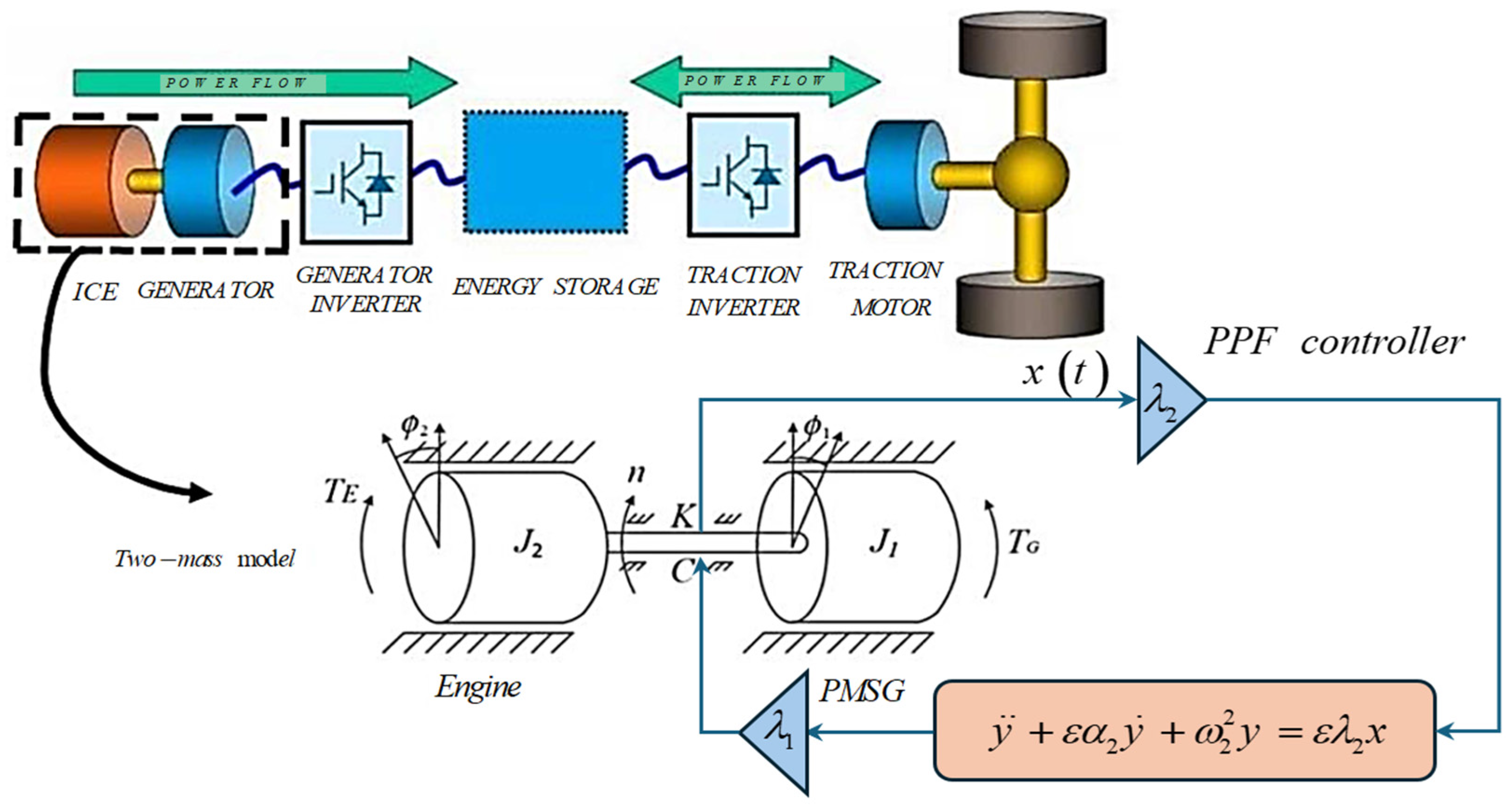
2. Closed Loop Model

2.1. System Dynamics without Control

The equation of motion of a one-degree-of-freedom series hybrid electric vehicle obtained by [6] is as follows:

$$\ddot{x}+\epsilon {\alpha }_1\dot{x}+{{\omega }_1}^{2}x+\epsilon \eta x^2+\epsilon \beta x^3+\epsilon \gamma x^4+2\mu x^5=\epsilon f\sin \left(2\omega t\right).$$

(1)

Figure 1 in a series hybrid electric vehicle, the engine, or power generator, directly charges the batteries or powers an electric motor.

2.2. System Dynamics with PPF Control

Figure 2 depicts a two-mass model and a schematic illustration of a series hybrid electric vehicle incorporating a PPF controller. $T_E$ denotes engine torque, $T_G$ denotes PMSG torque, $J_1$ denotes PMSG inertia, $J_2$ denotes engine inertia, ${\varphi }_1$ and ${\varphi }_2$ denote the torsional vibration angles at the shaft’s end under various excitations, where C represents the damping coefficient, and $K$ denotes equivalent shaft stiffness. $x$ is the displacement of the system. The damping factor epitomized by ${\alpha }_1$, The nonlinearities terms factors are $\eta ,\beta ,\gamma ,\mu$. The excitation frequency and amplitude are $\omega$ and $f$. ${\omega }_1$ is the natural frequency with the addition of the positive position feedback controller on the system.

The effective PPF controller design hinges on aligning its natural frequency, denoted as ${\omega }_1$ with both the external force frequency symbolized by $\omega$, while the natural frequency of the hybrid electric vehicles (HEVs) is represented by ${\omega }_2$. This synchronization is essential for achieving optimal performance and stability and enables the controller to accurately respond to the external force and the intrinsic dynamics of the HEVs system. However, when resonance conditions between the main system and the PPF controller are disrupted, the controller may inadvertently inject excessive vibrational energy into the main system instead of damping it.

Therefore, the equations of the motions of the system with PPF control found in Figure 2 can be constructed as follows:

$$\ddot{x}+\epsilon {\alpha }_1\dot{x}+{{\omega }_1}^{2}x+\epsilon \eta x^2+\epsilon \beta x^3+\epsilon \gamma x^4+2\mu x^5=\epsilon f\sin \left(2\omega t\right)+\epsilon {\lambda }_{1}y,$$

(2)

$$\ddot{y}+\epsilon {\alpha }_2\dot{y}+{{\omega }_2}^{2}y=\epsilon {\lambda }_{2}x.$$

(3)

3. Mathematical Investigations

3.1. Perturbation Analysis

This section employs the multiple scales perturbation technique to determine an ap-proximate solution for the nonlinear dynamical system controlled by the proposed PPF method outlined in Equations (2) and (3). This approach allows us to derive a first-order approximate solution, as detailed in references [25,26,27].

$$\begin{array}{l}t={\epsilon }^n{T}_n,\\ x(t;\epsilon )=x_0(T_0,T_1)+\epsilon x_1(T_0,T_1)+O({\epsilon }^2),\\ y(t;\epsilon )=y_0(T_0,T_1)+\epsilon y_1(T_0,T_1)+O({\epsilon }^2).\end{array}\}$$

(4)

Within this setting, the “fast scale” is represented by $T_0$, and the “slow scale” is denoted as $T_1=\epsilon t$. When employing (MTSM), the derivatives assume the following forms:

$$\begin{array}{l}{\displaystyle \frac{d}{dt}}=D_0+\epsilon D_1+{\epsilon }^2{D}_2+\dots ,\\ {\displaystyle \frac{d^2}{d{t}^2}}=D_0^2+2\epsilon D_0{D}_1+\dots ,\end{array}\} D_j={\displaystyle \frac{\partial }{\partial T_j}} (j=0,1).$$

(5)

Announcing equivalences (4) and (5) in Equations (2) and (3) such that

$$\begin{array}{ll}\left({D_0}^2+{{\omega }_1}^2\right)x_0+\epsilon \left({D_0}^2+{{\omega }_1}^2\right)x_1& =\epsilon f\sin \left(2\omega t\right)+ {\lambda }_1{y}_0-2D_0{D}_1{x}_0-{\alpha }_1{D}_0{x}_0-\eta {x_0}^2\\ & -\beta {x_0}^3-\gamma {x_0}^4-\mu {x_0}^5+O({\epsilon }^2),\end{array}$$

(6)

$$\left({D_0}^2+{{\omega }_2}^2\right)y_0+\epsilon \left({D_0}^2+{{\omega }_2}^2\right)y_1=\epsilon \left({\lambda }_2{x}_0-2D_0{D}_1{y}_0-{\alpha }_2{D}_0{y}_0\right)+O({\epsilon }^2).$$

(7)

Comparing the quantities of the same power of $\epsilon$:

$O({\epsilon }^0)$

$$({D_0}^2+{{\omega }_1}^2)x_0=0,$$

(8)

$$\left({D_0}^2+{{\omega }_2}^2\right)y_0=0.$$

(9)

$O(\epsilon )$

$$\left({D_0}^2+{{\omega }_1}^2\right)x_1=f\sin \left(2\omega t\right)+{\lambda }_1{y}_0-2D_0{D}_1{x}_0-{\alpha }_1{D}_0{x}_0-\eta {x_0}^2-\beta {x_0}^3-\gamma {x_0}^4-\mu {x_0}^5,$$

(10)

$$\left({D_0}^2+{{\omega }_2}^2\right)y_1={\lambda }_2{x}_0-2D_0{D}_1{y}_0-{\alpha }_2{D}_0{y}_0.$$

(11)

From Equations (8) and (9) Resolution the homogenous differential equations we obtain the following:

$$x_0(T_0,T_1)=A(T_1) e^{i{\omega }_1\left(T_0\right)}+\overline{A}(T_1) e^{-i{\omega }_1\left(T_0\right)},$$

(12)

$$y_0(T_0,T_1)=B(T_1) e^{i{\omega }_2\left(T_0\right)}+\overline{B}(T_1) e^{-i{\omega }_2\left(T_0\right)}.$$

(13)

Differentiate Equations (12) and (13) with respect to $t$ and submit in Equations (10) and (11).

$$\begin{array}{ll}\left({D_0}^2+{{\omega }_1}^2\right)x_1& =\left(-2i{\omega }_{1}DA-{\alpha }_{1}i{\omega }_{1}A-3\beta A^2\overline{A}-10\mu A^3{\overline{A}}^2\right)e^{i{\omega }_1(T_0)}-2\eta A\overline{A}\\ & -\left(\eta A^2+4\gamma A^3\overline{A}\right)e^{2i{\omega }_1(T_0)}+f\sin \left(2\omega t\right)+{\lambda }_{1}B{e}^{i{\omega }_2(T_0)}-6\gamma A^2{\overline{A}}^2\\ & -\left(\beta A^3+5\mu A^4\overline{A}\right)e^{3i{\omega }_1(T_0)}-4\gamma A^4{e}^{4i{\omega }_1(T_0)}-\mu A^5{e}^{5i{\omega }_1(T_0)}+C.C.,\end{array}$$

(14)

$$\left({D_0}^2+{{\omega }_2}^2\right)y_1={\lambda }_{2}A{e}^{i{\omega }_1(T_0)}-2i{\omega }_{2}DB{e}^{i{\omega }_2(T_0)}-i{\alpha }_2{\omega }_{2}B{e}^{i{\omega }_2(T_0)}+C.C.$$

(15)

The components that are complex conjugates are gathered in the term denoted as C.C.

After eliminating, the secular terms take the followings forms:

$$\left(-2i{\omega }_{1}DA-{\alpha }_{1}i{\omega }_{1}A-3\beta A^2\overline{A}-10\mu A^3{\overline{A}}^2\right)e^{i{\omega }_1(T_0)}+f\sin \left(2\omega t\right)+{\lambda }_{1}B{e}^{i{\omega }_2(T_0)}=0,$$

(16)

$$\left(-2i{\omega }_{2}DB-i{\alpha }_2{\omega }_{2}B\right)e^{i{\omega }_2(T_0)}+{\lambda }_{2}A{e}^{i{\omega }_1(T_0)}=0.$$

(17)

Based on the primary estimate, we determined the resonance cases that follow include

• SHR: $\omega \cong {\omega }_1/2$.
• IR: ${\omega }_1\cong {\omega }_2$.

3.2. Periodic Solutions

Then, we discuss the solvability conditions and introduce detuning parameters $({\sigma }_1)\&({\sigma }_2)$ to achieve:

$$\begin{array}{l}\omega ={\displaystyle \frac{1}{2}}{\omega }_1+\epsilon {\sigma }_1,\\ {\omega }_2={\omega }_1+\epsilon {\sigma }_2.\end{array}\}$$

(18)

Including Equation (18) the equation is divided into secular and small terms by separating (16) and (17). To gather the solvability conditions, the process involves:

$$\left(-2i{\omega }_{1}DA-{\alpha }_{1}i{\omega }_{1}A-3\beta A^2\overline{A}-10\mu A^3{\overline{A}}^2\right)+{\displaystyle \frac{f}{2i}}{e}^{2i{\sigma }_1{T}_1}+{\lambda }_{1}B{e}^{i{\sigma }_2{T}_1}=0,$$

(19)

$$-2i{\omega }_{2}DB-i{\alpha }_2{\omega }_{2}B+{\lambda }_{2}A{e}^{-i{\sigma }_2{T}_1}=0.$$

(20)

To scrutinize the key of (19) and (20) exchanging $A$ and $B$ by the polar form as follows:

$$A(T_1)={\displaystyle \frac{1}{2}}{a}_1(T_1) e^{i{\theta }_1(T_1)},DA(T_1)={\displaystyle \frac{1}{2}}\left({\dot{a}}_1(T_1) +i{a}_1(T_1){\dot{\theta }}_1(T_1)\right)e^{i{\theta }_1(T_1)},$$

(21)

$$B(T_1)={\displaystyle \frac{1}{2}}{a}_2(T_1) e^{i{\theta }_2(T_1)},DB(T_1)={\displaystyle \frac{1}{2}}\left({\dot{a}}_2(T_1) +i{a}_2(T_1){\dot{\theta }}_2(T_1)\right)e^{i{\theta }_2(T_1)}.$$

(22)

where $a_1$ and $a_2$ are the steady state phases and amplitudes of the motion of the system and controller, respectively, and the phases of motion are signified by ${\varphi }_1\&{\varphi }_2$. Inserting (21) and (22) into (19) and (20), upon calculation, the resulting equations governing amplitude and phase modulation are as follows:

$${\dot{a}}_1=-{\displaystyle \frac{1}{2}}{\alpha }_1{a}_1-{\displaystyle \frac{f}{2{\omega }_1}}\cos {\varphi }_1+{\displaystyle \frac{{\lambda }_1}{2{\omega }_1}}{a}_2\sin {\varphi }_2,$$

(23)

$$a_1{\dot{\theta }}_1={\displaystyle \frac{3}{8{\omega }_1}}\beta {a_1}^3+{\displaystyle \frac{5}{16{\omega }_1}}\mu {a_1}^5-{\displaystyle \frac{f}{2{\omega }_1}}\sin {\varphi }_1-{\displaystyle \frac{{\lambda }_1}{2{\omega }_1}}{a}_2\cos {\varphi }_2,$$

(24)

$${\dot{a}}_2=-{\displaystyle \frac{1}{2}}{\alpha }_2{a}_2-{\displaystyle \frac{{\lambda }_2}{2{\omega }_2}}{a}_1\sin {\varphi }_2,$$

(25)

$$a_2{\dot{\theta }}_2=-{\displaystyle \frac{{\lambda }_2}{2{\omega }_2}}{a}_1\cos {\varphi }_2.$$

(26)

where ${\varphi }_1=2{\sigma }_1{T}_1-{\theta }_1$ & ${\varphi }_2={\sigma }_2{T}_1+{\theta }_2-{\theta }_1$. To return to the major system parameters, consider the following equations:

$${\dot{a}}_1=-{\displaystyle \frac{1}{2}}{\alpha }_1{a}_1-{\displaystyle \frac{f}{2{\omega }_1}}\cos {\varphi }_1+{\displaystyle \frac{{\lambda }_1}{2{\omega }_1}}{a}_2\sin {\varphi }_2,$$

(27)

$$a_1{\dot{\varphi }}_1=2{\sigma }_1{a}_1-{\displaystyle \frac{3}{8{\omega }_1}}\beta {a_1}^3-{\displaystyle \frac{5}{16{\omega }_1}}\mu {a_1}^5+{\displaystyle \frac{f}{2{\omega }_1}}\sin {\varphi }_1+{\displaystyle \frac{{\lambda }_1{a}_2}{2{\omega }_1}}\cos {\varphi }_2,$$

(28)

$${\dot{a}}_2=-{\displaystyle \frac{1}{2}}{\alpha }_2{a}_2-{\displaystyle \frac{{\lambda }_2}{2{\omega }_2}}{a}_1\sin {\varphi }_2,$$

(29)

$$a_2{\dot{\varphi }}_2=({\sigma }_2-2{\sigma }_1)a_2+a_2{\dot{\varphi }}_1-{\displaystyle \frac{{\lambda }_2}{2{\omega }_2}}{a}_1\cos {\varphi }_2.$$

(30)

The control rule’s performance will be assessed by calculating the equilibrium solutions of (27), (28), (29) and (30) and assessing their stability as a function of the parameters ${\sigma }_1,{\sigma }_2,\eta ,\beta ,\gamma ,{\lambda }_1,{\lambda }_2$ and $f$.

3.3. A Certain Solution

We can potentially identify the steady-state solution fixed point of Equations (27)–(30) by inserting ${\dot{a}}_1={\dot{a}}_2={\dot{\varphi }}_1={\dot{\varphi }}_2=0$

$${\displaystyle \frac{1}{2}}{\alpha }_1{a}_1=-{\displaystyle \frac{f}{2{\omega }_1}}\cos {\varphi }_1+{\displaystyle \frac{{\lambda }_1}{2{\omega }_1}}{a}_2\sin {\varphi }_2,$$

(31)

$${\displaystyle \frac{3}{8{\omega }_1}}\beta {a_1}^3+{\displaystyle \frac{5}{16{\omega }_1}}\mu {a_1}^5-2a_1{\sigma }_1={\displaystyle \frac{f}{2{\omega }_1}}\sin {\varphi }_1+{\displaystyle \frac{{\lambda }_1}{2{\omega }_1}}{a}_2\cos {\varphi }_2,$$

(32)

$${\displaystyle \frac{1}{2}}{\alpha }_2{a}_2=-{\displaystyle \frac{{\lambda }_2}{2{\omega }_2}}{a}_1\sin {\varphi }_2,$$

(33)

$$\left({\sigma }_2-2{\sigma }_1\right)a_2={\displaystyle \frac{{\lambda }_2}{2{\omega }_2}}{a}_1\cos {\varphi }_2.$$

(34)

Squaring then adding both sides of Equations (33) and (34) to obtain the following one:

$$\left(4{{\omega }_2}^2{\left({\sigma }_2-2{\sigma }_1\right)}^2+{{\alpha }_2}^2{{\omega }_2}^2\right){a_2}^2={{\lambda }_2}^2{a_1}^2.$$

(35)

From (33) and (34), we have the following:

$$\cos {\varphi }_2={\displaystyle \frac{2{\omega }_2\left({\sigma }_2-2{\sigma }_1\right)a_2}{{\lambda }_2{a}_1}},$$

(36)

$$\sin {\varphi }_2=-{\displaystyle \frac{{\omega }_2{\alpha }_2{a}_2}{{\lambda }_2{a}_1}}.$$

(37)

Inserting (36) and (37) into (32) and (33), we obtain

$${\displaystyle \frac{f}{2{\omega }_1}}\cos {\varphi }_1=-{\displaystyle \frac{1}{2}}{\alpha }_1{a}_1-{\displaystyle \frac{{\lambda }_1{\omega }_2{\alpha }_2{a_2}^2}{2{\omega }_1{\lambda }_2{a}_1}},$$

(38)

$$\cos {\varphi }_1=-{\displaystyle \frac{2{\omega }_1}{f}}\left({\displaystyle \frac{{\lambda }_1{\omega }_2{\alpha }_2{a_2}^2}{2{\omega }_1{\lambda }_2{a}_1}}+{\displaystyle \frac{1}{2}}{\alpha }_1{a}_1\right),$$

(39)

$${\displaystyle \frac{f}{2{\omega }_1}}\sin {\varphi }_1={\displaystyle \frac{3}{8{\omega }_1}}\beta {a_1}^3+{\displaystyle \frac{5}{16{\omega }_1}}\mu {a_1}^5-2a_1{\sigma }_1-{\displaystyle \frac{{\lambda }_1{\omega }_2\left({\sigma }_2-2{\sigma }_1\right){a_2}^2}{{\omega }_1{\lambda }_2{a}_1}},$$

(40)

$$\sin {\varphi }_1=-{\displaystyle \frac{2{\omega }_1}{f}}\left(2a_1{\sigma }_1-{\displaystyle \frac{3}{8{\omega }_1}}\beta {a_1}^3-{\displaystyle \frac{5}{16{\omega }_1}}\mu {a_1}^5+{\displaystyle \frac{{\lambda }_1{\omega }_2\left({\sigma }_2-2{\sigma }_1\right){a_2}^2}{{\omega }_1{\lambda }_2{a}_1}}\right).$$

(41)

By squaring and summing the Equations (39) and (41), we obtain

$${\left(\begin{array}{l}2a_1{\sigma }_1-{\displaystyle \frac{3}{8{\omega }_1}}\beta {a_1}^3-{\displaystyle \frac{5}{16{\omega }_1}}\mu {a_1}^5-\\ +{\displaystyle \frac{{\lambda }_1{\omega }_2\left({\sigma }_2-2{\sigma }_1\right){a_2}^2}{{\omega }_1{\lambda }_2{a}_1}}\end{array}\right)}^2+{\left(-{\displaystyle \frac{{\lambda }_1{\omega }_2{\alpha }_2{a_2}^2}{2{\omega }_1{\lambda }_2{a}_1}}-{\displaystyle \frac{1}{2}}{\alpha }_1{a}_1\right)}^2={\displaystyle \frac{f^2}{4{{\omega }_1}^2}}.$$

(42)

Equations (35) and (42), known as the frequency response equations, are employed to explain how the system behaves in practical situations under steady-state conditions. These equations illustrate the system’s response across different frequencies when exposed to constant input signals. i.e., ($a_1\ne 0,a_2\ne 0$).

3.4. Stability Analysis via Linearizing the above System

The equilibrium solution’s stability was evaluated by analyzing the eigenvalues of the Jacobian matrix presented in Equations (27)–(30). Stability is assessed by focusing on the real components of these eigenvalues: if all eigenvalues exhibit a negative real part, the equilibrium solution is deemed asymptotically stable. Conversely, if any eigenvalue possesses a positive real component, the equilibrium solution is regarded as unstable. To provide further clarity on stability, the analysis initially involves examining small deviations from steady-state solutions to determine the stability criteria. This examination enables the understanding of the system’s response to small disturbances around the equilibrium $a_{10},a_{20},{\varphi }_{10}$ and ${\varphi }_{20}$. Thus, we assume that

$$\begin{array}{cc}{a}_1=a_{11}+a_{10},\hfill & a_2=a_{21}+a_{20},\\ {\varphi }_1={\varphi }_{11}+{\varphi }_{10},\hfill & {\varphi }_2={\varphi }_{21}+{\varphi }_{20},\\ {\dot{a}}_1={\dot{a}}_{11},\hfill & {\dot{a}}_2={\dot{a}}_{21},{\dot{\varphi }}_1={\dot{\varphi }}_{11},\\ {\dot{\varphi }}_2={\dot{\varphi }}_{21}.\hfill & \end{array}\}$$

(43)

where $a_{10},a_{20},{\varphi }_{10}$ and ${\varphi }_{20}$ satisfy (35) and (42). Also, $a_{11},a_{21},{\varphi }_{11}$ and ${\varphi }_{21}$ are perturbations assumed to be small compared to $a_{10},a_{20},{\varphi }_{10}$ and ${\varphi }_{20}$. Substituting (43) into (27)–(30), expanding for small $a_{11},a_{21},{\varphi }_{11}$ and ${\varphi }_{21}$, and keeping linear terms in $a_{11},a_{21},{\varphi }_{11}$ and ${\varphi }_{21}$, we obtain

$${\dot{a}}_{11}=r_{11}{a}_{11}+r_{12}{\varphi }_{11}+r_{13}{a}_{21}+r_{14}{\varphi }_{21},$$

(44)

$${\dot{\varphi }}_{11}=r_{21}{a}_{11}+r_{22}{\varphi }_{11}+r_{23}{a}_{21}+r_{24}{\varphi }_{21},$$

(45)

$${\dot{a}}_{21}=r_{31}{a}_{11}+r_{32}{\varphi }_{11}+r_{33}{a}_{21}+r_{34}{\varphi }_{21},$$

(46)

$${\dot{\varphi }}_{21}=r_{41}{a}_{11}+r_{42}{\varphi }_{11}+r_{43}{a}_{21}+r_{44}{\varphi }_{21}.$$

(47)

where $r_{ij},i=1,2,3,4$ and $j=1,2,3,4$ are given in the Appendix A.

Equations (43)–(46) can be presented in the following matrix form:

$${\left[{\dot{a}}_{11} {\dot{\varphi }}_{11}{\dot{a}}_{21} {\dot{\varphi }}_{21}\right]}^T=\left[J\right]{\left[a_{11} {\varphi }_{11}{a}_{21} {\varphi }_{21}\right]}^T,$$

(48)

$$\left[J\right]=\left[\begin{array}{l}{r}_{11} r_{12} r_{13} r_{14}\\ r_{21} r_{22} r_{23} r_{24}\\ r_{31} r_{32} r_{33} r_{34}\\ r_{41} r_{42} r_{43} r_{44}\end{array}\right].$$

(49)

where $\left[J\right]$ is the Jacobian matrix.

Therefore, the stability of the steady-state solutions is determined by examining the eigenvalues of the Jacobian matrix. This analysis yields the following eigenvalue equation:

$$\left|\begin{array}{cccc}{r}_{11}-\lambda & r_{12}& r_{13}& r_{14}\\ r_{21}& r_{22}-\lambda & r_{23}& r_{24}\\ r_{31}& r_{32}& r_{33}-\lambda & r_{34}\\ r_{41}& r_{42}& r_{43}& r_{44}-\lambda \end{array}\right|=0,$$

(50)

where the above polynomial has the following roots:

$${\lambda }^4+{\Gamma }_1{\lambda }^3+{\Gamma }_2{\lambda }^2+{\Gamma }_3\lambda +{\Gamma }_4=0,$$

(51)

where ${\Gamma }_i; (i=1,\dots ,4)$ are the coefficients of Equation (50) defined in the appendix. The Routh–Hurwitz criterion must be satisfied for the abovementioned system’s solution to be stable:

$${\Gamma }_1>0, {\Gamma }_1{\Gamma }_2-{\Gamma }_3>0,{\Gamma }_3({\Gamma }_1{\Gamma }_2-{\Gamma }_3)-{\Gamma }_1^2{\Gamma }_4>0,{\Gamma }_4>0.$$

(52)

4. Results and Discussion

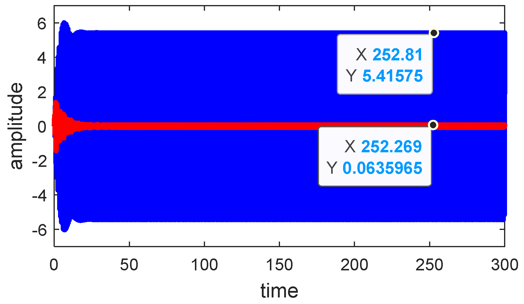
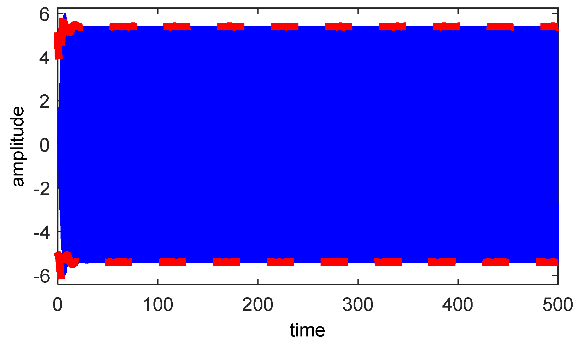
4.1. Effectiveness of PPF Control on Time History

We quantitatively investigated the system’s results using MATLAB’s (R2023b) “Ode 45” module. (MTSM) was also used to explain how different factors affected the behavior of the controlled system. This method has allowed investigation into how changes in certain parameters can affect the overall dynamics or performance of the system under control; Figure 2 depicts a schematic depiction and a simplified two-mass model of a series hybrid electric system [6]. In this section, a study is conducted to examine the steady-state responses of the primary system and its related controller. The examination focuses on several controller parameters under the situation of (SHR). This experimentation study resolves to establish the modifications in controller parameters that affect the system’s stability and performance in the 1:2 IR operational zone. The primary system’s results are plotted as steady-state amplitudes versus detuning parameters. Plotting figures requires the usage of the following system parameters.

$$\begin{array}{l}{\omega }_2={\omega }_1=10; \mu =0.01; \mathrm{f}=40; {\alpha }_1=0.5; {\alpha }_2=0.1; \omega =5; \gamma =0.005; \beta =0.005; \eta =0.0003; {\lambda }_1=25;\\ {\lambda }_2 =25.\end{array}$$

In Figure 3, the initial steady-state amplitudes of the basic system, before integrating PPF controllers, are depicted at approximately 5.41, representing the worst resonance case. Upon the incorporation of PPF controllers, the amplitudes of the primary system have notably decreased to a value of 0. 0635. This indicates that the efficacy of the PPF controllers is approximately 90%, resulting in a reduction in vibrations by roughly 99% compared to their levels without control.

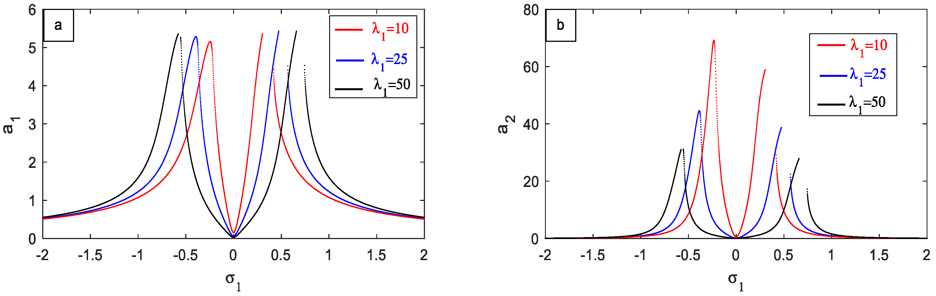
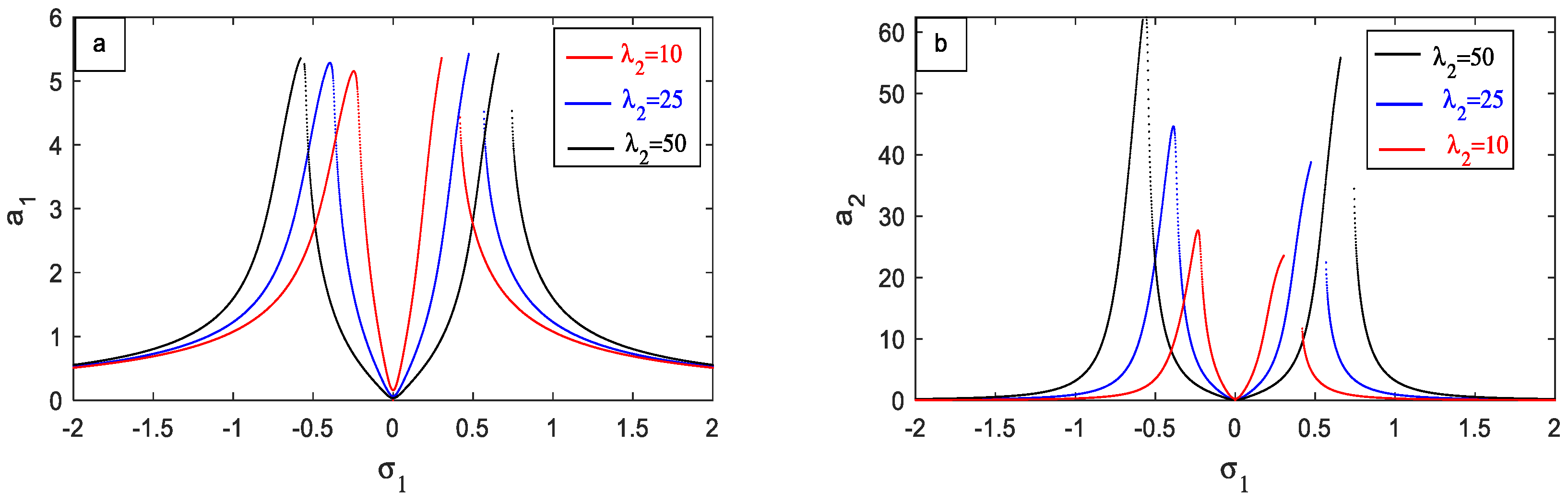
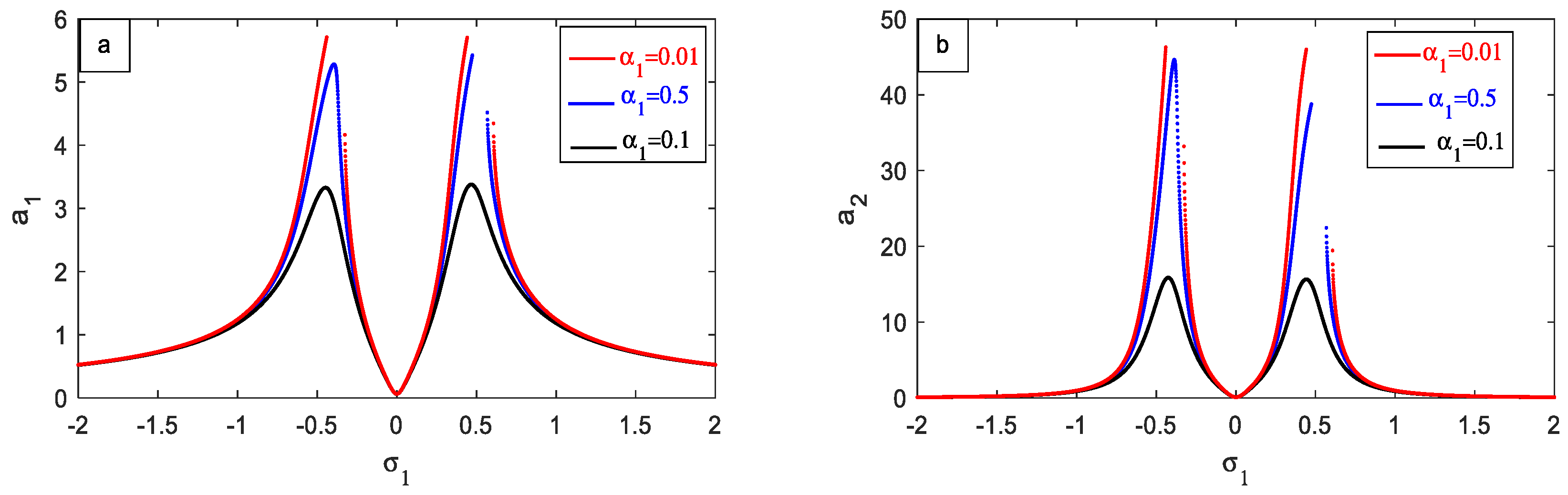
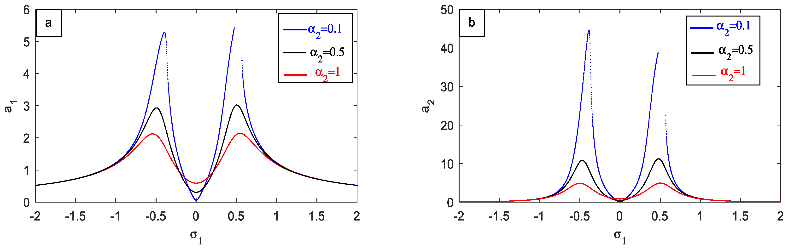
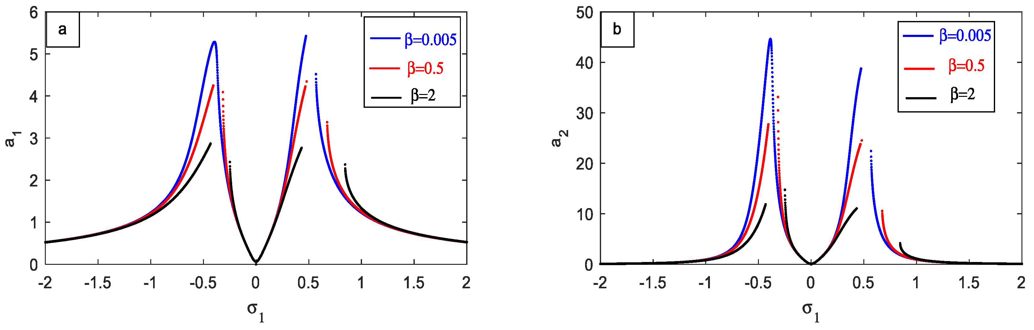
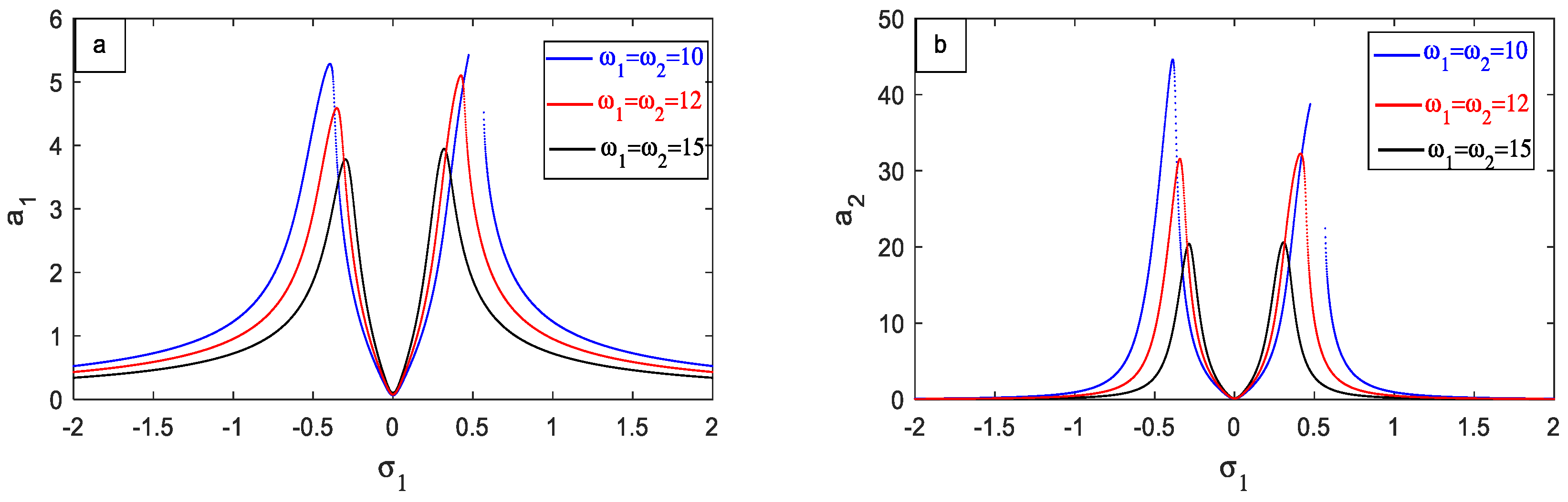
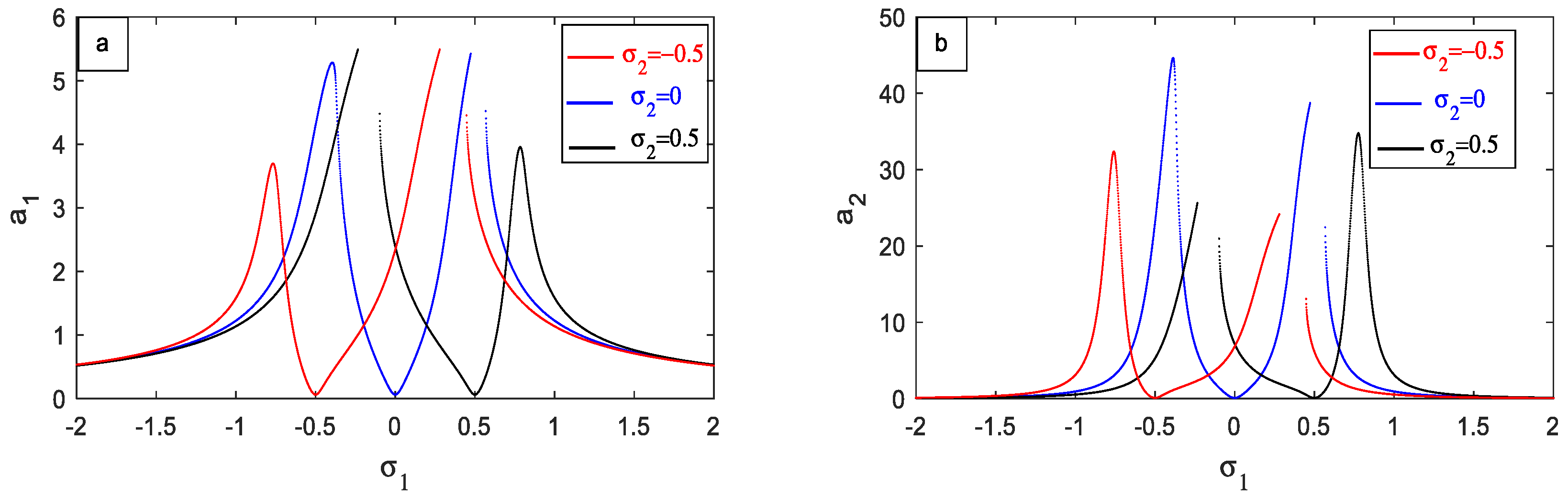
4.2. Frequency Response Curves (FRC)

The response amplitude is influenced by both the detuning parameter and the excitation amplitude $f$. Equations (35) and (42) are solved numerically and graphically to derive the solution for the amplitudes of all the main systems and the PPF controller at similar times. Figure 4, Figure 5, Figure 6, Figure 7, Figure 8, Figure 9, Figure 10, Figure 11, Figure 12, Figure 13 and Figure 14 are structured in two columns. The left column illustrates the capacity of the main system ($a_1$) on the vertical axis against the tuning parameter (${\sigma }_1$) on the horizontal axis. The right column similarly depicts the capacity of the control unit ($a_2$) on the vertical axis, also plotted against the tuning parameter (${\sigma }_1$) on the horizontal axis. The graphical solution is obtained concerning the detuning parameter, offering a visual depiction of how the amplitudes of these systems fluctuate as the detuning parameter ${\sigma }_1,{\sigma }_2$ changes two beaks are used to indicate this.

The frequency response curves depicted in Figure 4 exhibit the characteristics of the main system and the PPF controller. The frequency response of the controlled system is represented by a stable solution drawn as solid lines. Figure 4a depicts the frequency response curves of the main system, whereas Figure 4b shows the frequency response curves of the controller. These figures specify a visual comparison of how the systems perform at various frequencies and highlight the stability regions represented by the solid lines. We can conclude from this graph that the minimal value of the main system amplitude occurs at ${\sigma }_1=0$. This has implied that the PPF controller is intelligent in reducing main system vibrations in the super-harmonic resonance. The amplitudes of the main system and the PPF controller increase when the value of a harmonic excitation force grows, the jump phenomena happen, and the minimum value of the main system amplitude occurs at ${\sigma }_1=0$ as illustrated in Figure 5a,b.

The control signal gain ${\lambda }_1$ is represented in Figure 6a,b. It seems like a description of a series of results and observations related to the effects of the PPF controller and its parameters on the system behavior. The PPF controller’s amplitude shift to the right implies an expansion in the control signal’s bandwidth, as shown in Figure 6a. Figure 6b demonstrates that the PPF controller’s amplitude decreases monotonically, aligning with the intended purpose of the control signal gain.

Figure 7a,b depict the impact of the feedback signal ${\lambda }_2$; in Figure 7a, augmenting the feedback signal results in the vibration reduction frequency shift towards higher values for the controller. In Figure 7b, higher rates of the feedback signal have led to increased controller amplitudes.

Figure 8 illustrates the influence of the damping coefficient on the main system and the controller’s frequency response curves. Figure 8 shows that as ${\alpha }_1$ expands, the controller’s efficiency in deleting primary resonance excitations somewhat decreases, while the peak amplitudes of the main system and the controller decrease. Figure 9 shows that the damping coefficient ${\alpha }_2$ increases, and the controller’s effectiveness in mitigating super harmonic resonance excitations diminishes slightly, when both the main system and controller peak amplitudes decrease. Figure 10 demonstrates that the impact of the nonlinear parameters leads to an enhancement in the effectiveness of parameter $\beta$ whereas the vibration reduction frequency decreases. Figure 11 shows that when the effectiveness of parameter $\mu$ becomes higher, the vibration reduction frequency is decreasing. For small values of natural frequency for ${\sigma }_2=0$ i.e., (${\omega }_1={\omega }_2$), the peak amplitudes of both the main system and the PPF controller have shown an increase along with the expansion of the bandwidth for vibration reduction. Consequently, in scenarios where there is a low natural frequency, the PPF controller proves to be highly effective, as depicted in Figure 12. We select three distinct values of ${\sigma }_2$, the amplitude of the main system achieves its minimal value, as seen in Figure 13, when ${\sigma }_1={\sigma }_2$, which means that the PPF controller is more efficient in the resonance case.

5. Comparison

5.1. Comparison between Different Controllers with Time History Performance

Figure 14 illustrates the effectiveness of various control methods in mitigating vibrations under the most challenging conditions. The comparison encompasses positive position feedback (PPF), negative velocity (NVC), and propositional-derivative (PD) controllers. The results demonstrate that the PPF proves most effective in controlling and minimizing vibrations.

5.2. Comparison between Time History and Frequency Response Curves

Figure 15 demonstrates a strong agreement between the frequency response curves and the numerical solution obtained using RK-4. Figure 15a illustrates the previously mentioned comparison which discusses FRC from the main system’s capacity ($a_1$) with detuning parameter (${\sigma }_1$). Figure 15b depicts the previously mentioned comparison which discusses FRC from the control system’s capacity ($a_2$) with the tuning parameter (${\sigma }_1$). The above comparison results from Figure 15a,b can be summarized in

Table 1. Comparison of the results obtained for the FRC and RK-4 solution.

${\mathit{\sigma }}_{\mathbf{1}}$	RK-4 Solution	FRC	$\left|\mathit{R}\mathit{K}\mathbf{4} \mathit{S}\mathit{o}\mathit{l}\mathit{u}\mathit{t}\mathit{i}\mathit{o}\mathit{n}-\mathit{F}\mathit{R}\mathit{C}\right|$
−3	0.463124975460432	0.100187814076129	0.362937161384303
−2.7	0.463124975460483	0.111368846389836	0.351756129070647
−2.4	0.463124975460878	0.125367175821846	0.337757799639032
−2.1	0.463124975460678	0.143405678035335	0.319719297425343
−1.8	0.463124975460543	0.167538818881606	0.295586156578937
−1.5	0.463361256829522	0.201510240778341	0.261851016051181
−1.2	0.463124975460479	0.252961129489559	0.21016384597092
−0.9	0.463124975460708	0.340411579702025	0.122713395758683
−0.6	0.463124975460622	0.524477232033863	0.061352256573241
−0.3	0.463124975461229	1.22474096509607	0.761615989634841
0	0.463124975461430	0.063492063492063	0.399632911969367
0.3	0.463124975460857	1.226201951876355	0.763076976415498
0.6	0.463569183270159	0.524497879643075	0.060928696372916
0.9	0.463124975460831	0.340411579702025	0.122713395758806
1.2	0.463124975460638	0.252961129489559	0.210163845971079
1.5	0.463124975460543	0.201510240778341	0.261614734682202
1.8	0.463124975460607	0.167538818881606	0.295586156579001
2.1	0.463124975461053	0.100187814076129	0.362937161384924
2.4	0.463124975460740	0.111368846389836	0.351756129070904
2.7	0.463703390512664	0.125367175821846	0.338336214690818
3	0.463124975461298	0.143405678035335	0.319719297425963

.

5.3. Comparison between Analytical and Numerical Solutions before and after the Controller

Emphasizing the robust agreement and consistency observed between numerical simulations (solid line) and approximate solutions (dashed line) for the uncontrolled system and the system with the PPF controller.

Figure 16 showcases a significant correlation between the numerical and the approximate results for the uncontrolled system. This agreement underscores the compatibility and alignment of both methods in representing the behavior of the system without control. Furthermore, in Figure 17, a particularly strong correlation between numerical and approximate solutions is evident, specifically highlighting the impact of integrating the PPF controller into the system. This reinforces the reliability and consistency of both numerical simulations and approximate methods in depicting the system’s behavior when the PPF controller is implemented. While on one hand Figure 17a presents the previous comparison of the main system amplitude, on the other hand Figure 17b presents the same comparison but for the PPF controller amplitude. These observations underscore the robustness and accuracy of both numerical and approximate approaches in portraying the system’s behavior across various control scenarios, further validating their reliability in analyzing system dynamics.

5.4. Comparison with Previous Work

Reference [6] provides a comprehensive analysis of a nonlinear physical system within a series hybrid electric vehicle (SHEV) context. By closely examining the amplitude-frequency response curves (amplitude-FRCs), the study delves into the vibration properties of the new SHEV design. These amplitude-FRCs offer detailed insights into the stable and unstable motions of the SHEV. The investigation reveals the presence of multi-stability, with two or three distinct forms of attractors coexisting in the system. Furthermore, an analysis of the electromagnetic torque amplitude showcases additional dynamic regimes characterized by chaotic and periodic oscillations. Various phenomena such as hysteresis, period-doubling, and coexisting bifurcations with parallel branches are also identified. The study incorporates a Positive Position Feedback(PPF) controller into the system. By analyzing the time history and different parameters before and after the controller’s integration, it is observed that the system’s vibration is significantly reduced post-controller feedback addition, with the controller’s effectiveness $E_a$ ($E_a$ = amplitude without controller/amplitude with controller) reaching nearly 90. The amplitude of the vibrating system is lowered by approximately 98% compared to its value without control. Furthermore, there is a high degree of agreement between numerical and approximate solutions, enhancing the reliability and confidence in the analysis conducted.

6. Conclusions

Vehicle electrification has emerged as a definitive solution addressing air pollution issues in recent years; leading to a reduction in the reliance on non-renewable energy sources like gasoline that are commonly used in conventional vehicles. Including the various electrification options, hybrid electric vehicles (HEVs) have gained traction, particularly in the specialized domain of power distribution and transmission, they are often referred to as the HEV powertrain. HEVs utilize thermal and electrical energy sources to power their propulsion systems combining at least two distinct energy forms. In this paper, we aim to investigate the stability and behavior of the power generation set within the series equation of a hybrid electric vehicle.

To assess the viability conditions, we employed various time-scale techniques. We specifically utilized a Positive Position Feedback (PPF) controller in the Series Hybrid Vehicle (SHR) scenario to mitigate vibrations within the main system. These investigations were carried out using the MATLAB application. Throughout our analysis, we showcased the efficacy of different PPF controller gains while examining various settings. Our findings have emphasized the superiority of numerical solutions over approximate ones in accurately capturing the system’s behavior and stability characteristics. The analysis of hybrid electric vehicle powertrain stability findings are as follows:

Our research focuses on using a positive position feedback controller to improve the stability of a Series Hybrid Vehicle powertrain, particularly in mitigating vibrations. Here is a breakdown of our key findings:

• In order to design the PPF controller effectively, it is essential to adjust its natural frequency, denoted as ${\omega }_2$, to match the frequencies of both the external force, represented by $\omega$, and the natural frequency of the (HEVs), denoted as ${\omega }_1$. This alignment ensures the optimal performance and stability of the controller in response to the external force and the inherent dynamics of the (HEVs) system.
• The positive position feedback (PPF) controller demonstrates notable effectiveness in mitigating high-amplitude vibrations within nonlinear systems.
• The SHR and IR case $\omega \cong {\displaystyle \frac{1}{2}}{\omega }_1$ & ${\omega }_1={\omega }_2$ is one of the vibrating system’s most severe resonance cases.
• The amplitude of the vibrating system has decreased by approximately 98% after utilizing the PPF feedback controller compared to its value without control.
• The effectiveness of the PPF feedback controller, denoted as Ea_., reaches approximately 90, showcasing its high efficacy in controlling the system’s behavior.
• The response or behavior of the controlled system intensifies with the escalation of the external excitation force $f$.
• The response of the main system has decreased with increasing the natural frequency ${\omega }_1$.
• The curves are shifted to right with increasing the value of the PPF parameter ${\lambda }_1$, which is advantageous in the performance of the PPF controller.
• For the PPF parameter, the amplitude of the controlled system decreases very slowly.
• The solutions obtained from the frequency response curves (FRC) align well with those derived from the Runge–Kutta 4th order (RK-4) method.
• The closed loop response of relative displacement is obtained with PPF controller which comprises the peak-overshoot.
• The modified structure of the PPF controller is used for the control of relative displacement of suspension system. From the results, the PPF controller provided better closed loop performance in terms peak overshoot and settling time are minimized.

Overall Impression:

Our findings provide valuable insights into the stability characteristics of HEV powertrains and the effectiveness of using a PPF controller for vibration mitigation. The systematic analysis and validation of our results strengthen the significance of our research.

References

1. Wang, H.; Huang, Y.; Khajepour, A.; Zhang, Y.; Rasekhipour, Y.; Cao, D. Crash mitigation in motion planning for autonomous vehicles. IEEE Trans. Intell. Transp. Syst. 2019, 20, 3313–3323. [Google Scholar] [CrossRef]
2. Matharu, H.S.; Girase, V.; Pardeshi, D.B.; William, P. Design and deployment of hybrid electric vehicle. In Proceedings of the 2022 International Conference on Electronics and Renewable Systems (ICEARS), Tuticorin, India, 16–18 March 2022; pp. 331–334. [Google Scholar]
3. Belkhier, Y.; Oubelaid, A.; Shaw, R.N. Hybrid power management and control of fuel cells-battery energy storage system in hybrid electric vehicle under three different modes. Energy Storage 2024, 6, e511. [Google Scholar] [CrossRef]
4. Al Hla, Y.A.; Othman, M.; Saleh, Y. Optimizing an eco-friendly vehicle routing problem model using regular and occasional drivers integrated with driver behavior control. J. Clean. Prod. 2019, 234, 984–1001. [Google Scholar] [CrossRef]
5. Rajagopal, K.; Hussain, I.; Rostami, Z.; Li, C.; Pham, V.T.; Jafari, S. Magnetic induction can control the effect of external electrical stimuli on the spiral wave. Appl. Math. Comput. 2021, 390, 125608. [Google Scholar] [CrossRef]
6. Tame tang Meli, M.I.; Leutcho, G.D.; Yemele, D. Multistability analysis and nonlinear vibration for generator set in series hybrid electric vehicle through electromechanical coupling. Chaos: Interdiscip. J. Nonlinear Sci. 2021, 31, 073126. [Google Scholar] [CrossRef]
7. Shen, Z.; Luo, C.; Dong, X.; Lu, W.; Lv, Y.; Xiong, G.; Wang, F.Y. Two-Level Energy Control Strategy Based on ADP and A-ECMS for Series Hybrid Electric Vehicles. IEEE Trans. Intell. Transp. Syst. 2022, 23, 13178–13189. [Google Scholar] [CrossRef]
8. Wang, J.; Yang, H. Low carbon future of vehicle sharing, automation, and electrification: A review of modeling mobility behavior and demand. Renew. Sustain. Energy Rev. 2023, 177, 113212. [Google Scholar] [CrossRef]
9. Alatise, O.; Deb, A.; Bashar, E.; Ortiz Gonzalez, J.; Jahdi, S.; Issa, W. A Review of Power Electronic Devices for Heavy Goods Vehicles Electrification: Performance and Reliability. Energies 2023, 16, 4380. [Google Scholar] [CrossRef]
10. Smith, D.; Ozpineci, B.; Graves, R.L.; Jones, P.T.; Lustbader, J.; Kelly, K.; Mosbacher, J. Medium-and Heavy-Duty Vehicle Electrification: An Assessment of Technology and Knowledge Gaps (No. ORNL/SPR-2020/7); Oak Ridge National Lab. (ORNL): Oak Ridge, TN, USA; National Renewable Energy Lab. (NREL): Golden, CO, USA, 2020.
11. Amer, Y.A.; EL-Sayed, A.T.; Abd EL-Salam, M.N. On controlling of vibrations of a suspended cable via positive position feedback controller. Int. J. Dyn. Control 2023, 11, 370–384. [Google Scholar] [CrossRef]
12. He, C.; Tian, D.; Moatimid, G.M.; Salman, H.F.; Zekry, M.H. Hybrid rayleigh–van der pol–duffing oscillator: Stability analysis and controller. J. Low Freq. Noise Vib. Act. Control. 2022, 41, 244–268. [Google Scholar] [CrossRef]
13. Jamshidi, R.; Collette, C. Optimal negative derivative feedback controller design for collocated systems based on H2 and H∞ method. Mech. Syst. Signal Process. 2022, 181, 109497. [Google Scholar] [CrossRef]
14. Saeed, N.A.; El-Shourbagy, S.M.; Kamel, M.; Raslan, K.R.; Aboudaif, M.K. Nonlinear dynamics and static bifurcations control of the 12-pole magnetic bearings system utilizing the integral resonant control strategy. J. Low Freq. Noise Vib. Act. Control 2022, 41, 1532–1560. [Google Scholar] [CrossRef]
15. Ebrahimi, F.; Ahari, M.F. Active vibration control of the multilayered smart nanobeams: Velocity feedback gain effects on the system’s behavior. Acta Mech. 2024, 235, 493–510. [Google Scholar] [CrossRef]
16. Kandil, A.; Hamed, Y.S.; Alsharif, A.M. Rotor active magnetic bearings system control via a tuned nonlinear saturation oscillator. IEEE Access 2021, 9, 133694–133709. [Google Scholar] [CrossRef]
17. Saeed, N.A.; Awrejcewicz, J.; Elashmawey, R.A.; El-Ganaini, W.A.; Hou, L.; Sharaf, M. On 1/2-DOF active dampers to suppress multistability vibration of a 2-DOF rotor model subjected to simultaneous multiparametric and external harmonic excitations. Nonlinear Dyn. 2024, 112, 12061–12094. [Google Scholar] [CrossRef]
18. Amer, Y.A.; El-Sayed, A.T.; Abdel-Wahab, A.M.; Salman, H.F. Positive position feedback controller for nonlinear beam subject to harmonically excitation. Asian Res. J. Math. 2019, 12, 1–19. [Google Scholar] [CrossRef]
19. El-Shourbagy, S.M.; Saeed, N.A.; Kamel, M.; Raslan, K.R.; Abouel Nasr, E.; Awrejcewicz, J. On the performance of a nonlinear position-velocity controller to stabilize rotor-active magnetic-bearings system. Symmetry 2021, 13, 2069. [Google Scholar] [CrossRef]
20. Bauomy, H.; Taha, A. Nonlinear saturation controller simulation for reducing the high vibrations of a dynamical system. Math. Biosci. Eng. 2022, 19, 3487–3508. [Google Scholar] [CrossRef]
21. Moatimid, G.M.; El-Sayed, A.T.; Salman, H.F. Different controllers for suppressing oscillations of a hybrid oscillator via non-perturbative analysis. Sci. Rep. 2024, 14, 307. [Google Scholar] [CrossRef] [PubMed]
22. Bauomy, H. Safety action over oscillations of a beam excited by moving load via a new active vibration controller. Math. Biosci. Eng. 2023, 20, 5135–5158. [Google Scholar] [CrossRef]
23. Amer, Y.A.; Abd EL-Salam, M.N.; EL-Sayed, M.A. Behavior of a Hybrid Rayleigh-Van der Pol-Duffing Oscillator with a PD Controller. J. Appl. Res. Technol. 2022, 20, 58–67. [Google Scholar]
24. Hamed, Y.S.; Alotaibi, H.; El-Zahar, E.R. Nonlinear vibrations analysis and dynamic responses of a vertical conveyor system controlled by a proportional derivative controller. IEEE Access 2020, 8, 119082–119093. [Google Scholar] [CrossRef]
25. Kevorkian, J.; Cole, J.D.; Kevorkian, J.; Cole, J.D. The method of multiple scales for ordinary differential equations. In Multiple Scale and Singular Perturbation Methods; Springer: Berlin/Heidelberg, Germany, 1996; pp. 267–409. [Google Scholar]
26. Nayfeh, A. Perturbation Methods; Wiley: New York, NY, USA, 1973. [Google Scholar]
27. Dukkipati, R.V. Solving Vibration Analysis Problems Using Matlab; New Age International Pvt Ltd. Publishers: Delhi, India, 2007. [Google Scholar]
Figure 1. Diagram of the series hybrid electric vehicle.
Applsci 14 07215 g001
Figure 2. A two-mass model and a schematic illustration of a series hybrid electric vehicle [6].
Applsci 14 07215 g002
Figure 3. The amplitude of the main system before and after adding a positive position feedback (PPF) controller.
Applsci 14 07215 g003
Figure 4. Frequency resonance curves of (a) main system and (b) PPF controller.
Applsci 14 07215 g004
Figure 5. The effectiveness of the external excitation force f on (a) the main system (b) the PPF controller.
Applsci 14 07215 g005
Figure 6. The effectiveness of control signal gain λ 1 on (a) the main system (b) the PPF controller.
Applsci 14 07215 g006
Figure 7. The effectiveness of feedback signal λ 2 on (a) the main system (b) the PPF controller.
Applsci 14 07215 g007
Figure 8. The effectiveness of damping parameter α 1 on (a) the main system (b) the PPF controller.
Applsci 14 07215 g008
Figure 9. The effectiveness of damping parameter α 2 on (a) the main system (b) the PPF controller.
Applsci 14 07215 g009
Figure 10. The effectiveness of nonlinear parameter β on (a) the main system (b) the PPF controller.
Applsci 14 07215 g010
Figure 11. The effectiveness of the nonlinear parameter μ on (a) the main system (b) the PPF controller.
Applsci 14 07215 g011
Figure 12. Effect of varying the natural frequency ( ω 1 = ω 2 ) for σ 2 = 0 on the frequency response curves of (a) the main system (b) the PPF controller.
Applsci 14 07215 g012
Figure 13. Effect of varying σ 2 on the frequency response curves of (a) the main system (b) the PPF controller.
Applsci 14 07215 g013
Figure 14. Effect between the different types of controllers (PPF-NVC-PD).
Applsci 14 07215 g014
Figure 15. Comparison between FRC: from approximate solution (solid line) and RK-4 numerical solution (Green Circle) (a) the main system (b) the PPF controller.
Applsci 14 07215 g015
Figure 16. Comparison between approximate solution (dashed line) and numerical solution (solid line) for the vibration amplitude of uncontrolled main system.
Applsci 14 07215 g016
Figure 17. Comparison between approximate solution (dashed line) and numerical solution (solid line) for the vibration amplitude of (a) the main system (b) the PPF controller.
Applsci 14 07215 g017