Abstract
Ocean circulation plays an important role in the formation and occurrence of extreme climate events. The study shows that the periodic variation of ocean circulation under strong wind stress is closely related to climate oscillation. Ocean circulation is a nonlinear dynamic system, which shows complex nonlinear characteristics, so the essence behind ocean circulation has not been clearly explained. Therefore, the response and evolution of the circulation system to wind stress are studied based on the bifurcation and catastrophe theories in nonlinear dynamics. First, the quasi-geostrophic gyre equation and the normalized gravity model are introduced and developed to study ocean circulation driven by wind stress, and solved using the Galerkin method. Then, the bifurcation and catastrophe behaviors of the system governed by the low-order ocean circulation model during the change in wind stress intensity and the coexistence of multiple equilibria in the circulation system are studied in detail. The results show that saddle and unstable nodes appear in the system after a cusp catastrophe. With the change in model parameters, the unstable node becomes the unstable focus, and then the subcritical Hopf bifurcation occurs. The system forms a bistable interval when the system undergoes a catastrophe twice, and the system shows hysteresis. In addition, multiple equilibrium states are coexisting in the circulating system, and the unstable equilibrium state always changes into a stable equilibrium state through vortex movement. Therefore, there is a route for the system to induce short-term climate oscillation, that is, in the multi-stable equilibrium state of the system, the vortex oscillates after being subject to small disturbances, and then triggers climate oscillation.
1. Introduction
Ocean circulation is a fundamental component of Earth’s climate system, influencing weather patterns and contributing to the development of extreme climate events. Currently, the nature of ocean circulation and its evolution on time scales ranging from several months to several years are critical issues in oceanography [1]. Ocean circulation exhibits several distinct features. For instance, the thickness of the boundary layer formed by the atmosphere on the sea surface is greater due to the significantly lower density of wind-driven circulation compared with seawater [2]. Under the influence of wind stress, atmospheric momentum is transferred to the water body, causing the water to move along with the wind. Notable examples of this phenomenon are the Kuroshio in the North Pacific and the Gulf Stream in the North Atlantic, which represent the major western boundary currents in the Northern Hemisphere [1,3,4].
Historically, much of our understanding of ocean circulation was derived from observations. In 1898, Nansen, a Norwegian scientist, was likely the first to qualitatively describe the formation process of wind-driven circulation. According to his theories, wind stress acts upon the sea surface, transferring kinetic energy into the water body and causing surface water movement. He also observed that, in the Northern Hemisphere, the flow shifts to the right of the wind direction due to the Coriolis force. Subsequent theoretical research can be traced back to Ekman, who quantitatively described wind-driven circulation and studied the circulation structure within the sea surface boundary layer [5]. Ekman’s theory suggests that velocity within the boundary layer exhibits a spiral distribution, with the flow direction deviating to the right of the wind stress. This boundary layer has since been termed the Ekman layer. However, Ekman’s model assumes that wind stress on seawater acts solely as a frictional force, which does not fully align with actual observations. In 1947, building on Ekman’s quantitative model, Sverdrup considered the horizontal pressure gradient force in the wind-driven circulation model, establishing the relationship between basin-wide circulation and the wind stress curl [6]. Although Sverdrup innovatively proposed the formation process of wind-driven ocean circulation, he did not account for the western boundary effect (such as the formation of the Atlantic Gulf Stream, which includes the western boundary effect).
Based on previous theoretical frameworks and actual wind field characteristics, Munk introduced lateral friction in his model to represent the western boundary effect [3]. This model was later refined by Charney, who developed the inertial western boundary layer theory [7]. The series of studies conducted in the mid-20th century significantly deepened our understanding of ocean circulation. However, the spatial distribution of wind-driven circulation and the evolution of ocean currents were not accurately characterized due to the limitations of computing technology at the time. Pedlosky and Gill synthesized the results of previous research on geophysical flows, starting from the three-dimensional spherical rotation equations, and simplified the barotropic quasi-geostrophic model and the shallow water model [8,9]. Subsequent research on geophysical fluid dynamics has since been based heavily on their foundational work.
In the atmosphere–ocean system, the ocean serves as the largest reservoir of heat and water, with the movement of ocean currents exerting a significant impact on the climate of coastal areas, particularly on temperature and precipitation. The most direct meteorological manifestation of changes in ocean circulation is short-term climate oscillation. The study of this phenomenon is crucial, as common weather models, constrained by computational resources, are often inadequate for predicting climate changes over longer time scales. This limitation can lead to large-scale natural disasters when extreme climate events occur [10]. Two of the most significant examples are the El Niño Southern Oscillation in the equatorial Pacific and the Atlantic multi-decadal oscillation in the North Atlantic [11,12]. Indeed, the study of the El Niño–Southern Oscillation (ENSO) has long been a central topic in ocean and atmospheric sciences, with particular focus on the relationship between oceanic and atmospheric variables, their spatial structures, and temporal evolution.
By analyzing the singular frequency spectrum of various global average temperature records, it has been shown that the ocean surface temperature in the North Atlantic exhibits inter-annual variability [11]. Through spectral analysis, Delworth and Mann identified distinct spectral peaks within the 50–70 year frequency band [13]. This short-term climate oscillation in the Atlantic Ocean is termed the Atlantic multi-decadal oscillation (AMO), with the AMO index defined as the 10-year running average of ocean surface temperature, exhibiting an anomalous trend north of the equator. Interestingly, results indicate a strong negative correlation between AMO and precipitation across the continental United States. Specifically, during periods of a high (low) AMO index, precipitation is reduced (increased) across much of central United States [14,15]. McCarthy’s research demonstrates that the evolution of ocean circulation between the subtropical and subpolar zones can influence the development of AMO, and a negative AMO has been closely linked to the accelerated sea level rise along the northeast coast of the United States [12]. Consequently, some researchers suggest that inter-annual periodic climate changes in the atmosphere–ocean system are highly correlated with the influence of external atmospheric wind fields on ocean circulation [16].
In addition, the marginal seas, such as the South China Sea, exhibit evident characteristics of low-frequency periodic oscillation. Yang and Wu studied the climate evolution characteristics of the South China Sea using a two-layer quasi-geostrophic model, and found that the periodic behavior of the local climate is closely related to monsoonal patterns. They concluded that the monsoon first influences the evolution of ocean circulation, thereby inducing periodic climate oscillations [17]. The Kuroshio Extension (KE), an extension of the Kuroshio warm current in the North Pacific Ocean, is the region with the highest gyre kinetic energy in the North Pacific [4]. Observations indicate that the large-scale periodic oscillation of the KE can transport high-temperature, high-salinity seawater from the Pacific Ocean to coastal areas, affecting the meteorology and hydrology of North America’s coastal regions, leading to abnormally high temperatures [18,19].
The broader impact of wind on climate systems and ocean circulation has also been a focal point of recent studies. Liang examined how low- and mid-level wind couplings and topography affect mesoscale convective systems (MCSs) in Northwest China, discovering that low-level anticyclonic circulation impacts the distribution of high humidity zones [20]. Clancy et al. analyzed Arctic cyclones, identifying asymmetries in atmospheric and sea ice structures that resemble mid-latitude cyclones with distinct warm and cold sectors [21]. Zuo and Hasager assessed the impact of Aeolus wind data on near-surface wind forecasts, noting positive effects in high-latitude regions, particularly with extended forecast time steps [22]. McMonigal et al. investigated the effects of wind-driven ocean circulation on global warming, finding that these changes amplified the warming rate by 17% from 1979 to 2014, underscoring the importance of atmospheric circulation changes for accurate climate predictions [23]. Li et al. (2023) explored tropical cyclone (TC) wind forcing within a fully coupled climate model, demonstrating that TCs increase ocean heat content through effects on vertical mixing, air–sea enthalpy fluxes, and cloud cover [24].
From an ocean dynamics perspective, Paldor and Friedland (2023) extended Ekman’s wind-driven transport theory to the plane by introducing pseudo-angular momentum, which simplifies the understanding of water column trajectories near the equator [25]. Kong and Jansen (2021) emphasized the role of ocean topography in modulating Southern Ocean circulation responses to wind stress changes, demonstrating that stationary eddies play a dominant role in these responses [26]. Additionally, Thomsen et al. (2021) found that eddy effects generally counteract Ekman circulation, with changes in air–sea heat flux influencing the strength of eddy cancellation. Specifically, as heat flux increases, eddy cancellation decreases, causing the flow to gradually approach classical Ekman circulation [27].
To explore the nature of ocean circulation evolution, scholars have developed an idealized multi-gyre model, grounded in the study of wind-driven circulation. In a confined fluid region, the system satisfies the governing equations of quasi-geostrophic (QG) or shallow water (SW) dynamics under a normalized gravity mode. When the system is forced by a wind field composed of multiple gyres, these gyres can represent subpolar cyclones and subtropical anticyclones, which correspond to ocean gyres in the real-world ocean environment. Consequently, such an idealized gyre model has been widely applied in studies of large-scale mid-latitude ocean circulation responses to wind forcing [28,29,30].
In conjunction with the wind-driven circulation model and actual observational data, statistical analysis methods have been extensively utilized to study complex ocean currents. Methods such as empirical orthogonal function (EOF) analysis [31] and nonlinear time series analysis [32,33] have proven effective in climate change and oceanographic research. However, a limitation of these methods is the need for additional models to establish causal relationships between key physical quantities. Moreover, statistical integral quantities are often used to analyze interactions between mean physical quantities and perturbations [8]. Nonetheless, the complexity of most ocean circulation problems often results in significant deviations in statistical integrals, as observational or ocean models may not fully satisfy the necessary conditions.
As discussed earlier, certain behaviors of ocean circulation exhibit dynamic properties, making it feasible to study these systems from a dynamical perspective. Bryan and Holland identified that inter-annual phenomena in the ocean–atmosphere system’s climate change process possess dynamic characteristics [34,35]. In open ocean areas, Kondrashov analyzed gyres using adaptive harmonic decomposition and inverse stochastic modeling techniques, revealing that wind-driven ocean circulation exhibits quasi-periodic variations [28]. Indeed, understanding the evolution of ocean circulation by examining its sensitivity to various parameters using dynamic system theories is crucial. Since the 1990s, the dynamical system perspective has been introduced into oceanography, with researchers employing bifurcation theory from nonlinear dynamics to explain low-frequency periodic oscillations in ocean circulation [36]. Nonlinear dynamic theory suggests that low-frequency oscillations in the ocean are driven by attractors within the system, such as limit cycles, strange attractors, and homoclinic orbits [37,38].
The results from quasi-geostrophic (QG) models have been instrumental in explaining the asymptotic behavior of the shallow water system. Primeau’s investigation of a low-order quasi-geostrophic ocean circulation model revealed the presence of multiple equilibrium solutions, periodic solutions, and quasi-periodic solutions within the circulation system [39]. Notably, it was found that the circulation system can exhibit multiple equilibrium states. Through the stability analysis of nonlinear dynamics, it was determined that the system can possess both stable and unstable equilibria under identical parameters, where the circulation system in an unstable state will oscillate until it reaches a stable equilibrium [40]. Simonnet’s work demonstrated that the overall system maintains antisymmetry as long as the zonal wind stress is symmetric. However, as the wind stress intensifies and more energy is injected into the system, the symmetry of the circulation system can break, leading to the emergence of multiple equilibria [41]. Sheremet studied the Rossby resonance modes under single and double vortex wind stress, finding that the motion of vortices within the circulation system exhibits periodic variation characteristics following the system’s bifurcation, with vortices changing periodically as wind stress further increases [42]. Dijkstra and Katsman also posited that asymmetric oscillation modes are inherent in the circulation system, and a Hopf bifurcation occurs as wind stress increases [41,43].
Interestingly, Simonnet and Ghil discovered a homoclinic bifurcation by increasing lateral friction in the original antisymmetric model and by adding two higher-order meridional modes to the low-order simplified model. They identified the homoclinic bifurcation as a primary cause of irregular changes within the circulation system [41].
To gain a deeper understanding of the influence of ocean circulation on climate anomalies, it is crucial to examine the bifurcation and catastrophic behaviors of low-order circulation models as wind stress intensity changes. In subsequent studies, the quasi-geostrophic gyre equation, coupled with a normalized gravity model, will be employed to describe wind-driven ocean circulation. The Galerkin method will be introduced to approximate the solution. The nonlinear dynamics of ocean circulation, from stability to instability under varying wind stress, will be analyzed in detail. The findings of this research will hold significant implications for the prediction and prevention of extreme climate events.
2. Galerkin Procedure
Large-scale numerical simulation and analysis represent the most economical and effective approach to studying the infinite-dimensional dynamical systems composed of continuum media, which exhibit a rich variety of nonlinear behaviors. However, when simplifying such systems using classical linearization methods, some nonlinear behaviors may not be accurately captured [3]. The direct numerical integration method is commonly employed to investigate dissipative infinite-dimensional dynamical systems, particularly those of second order in time. Nevertheless, simulating the long-term behavior of these systems demands substantial computational resources [44]. Consequently, it is crucial to reduce the complexity of the system by decreasing the number of degrees of freedom.
In reality, the long-term dynamical behaviors of an infinite-dimensional dissipative dynamical system are often attracted to an invariant manifold of finite dimension. By projecting the solution of the governing equations onto this invariant manifold, the system can be significantly simplified. Therefore, the Galerkin procedure is introduced as a method to approximate the solution of the system [45].
Considering the nonlinear equation,
where is a mapping on and boundary corresponds to region , and is given. The eigenfunction set of the linear operator with orthogonality is selected, so u can be expressed as,
where is an unknown variable. There will be residuals generated from the corresponding differential equation and boundary conditions, Equation (1).
Considering the basis function set , the Galerkin procedure requires the weighted integral of residual Equation (3) over and to satisfy the relationship,
Then, a series of simple algebraic equations can be obtained and variables can be obtained simultaneously. Furthermore, the desired variable u can be obtained.
3. Governing Equations of Ocean Circulation
In geophysical fluid dynamics, Pedlosky and Gill proposed the shallow water (SW) equations, and simplified the equations with the different environments, having a profound impact on the quantitative analysis [8,9]. This paper mainly studies the ocean circulation driven by wind. The Rossby number corresponding to the SW model is very small, and the topological change at the bottom of the calculation area is also very small. In this case, the SW model can be simplified by assuming a small Rossby number. A single-layer quasi-geostrophic vorticity equation in a square region is obtained, using the equalization dimensionalization of characteristic flow rates and characteristic scales with the quasi-geostrophic theory.
where u and v denote the horizontal and vertical velocities, respectively. is the flow function, and is the vertical relative vorticity. and represent the horizontal and vertical wind stresses, respectively. In addition, Equation (7) shows the dimensionless parameters in Equation (5).
where is the Planetary vorticity gradient strength, F is the Rotating Froude number, is the Reynolds number, is the bottom friction coefficient, is the wind stress intensity, is the relative inertial boundary layer thickness, is the relative horizontal viscous boundary layer thickness, and is the relative vertical viscous boundary layer thickness. The dimensional parameters are listed in Table 1, and the values of these parameters refer to the settings in reference [17].

Table 1.
Dimensional parameters.
The normalized gravitational acceleration can be obtained by . The value in Ref. [17] is used, and the corresponding dimensionless parameters are given in Table 2, and the values of these parameters also refer to the settings in reference [17].
Table 2.
Dimensionless parameters.
It is worth noting that the velocity field of flow is expressed as a stream function in the field of geophysical fluid dynamics,
In the square region , Equation (5) satisfies the non-slip boundary condition and no penetration boundary condition, that is,
Also, for Equation (5), the system with respect to the central axis is antisymmetric without the wind stress term, and the relationship can be expressed as,
where the selection of will satisfy the antisymmetric relationship.
4. Results and Analysis
Based on the classic quasi-geostrophic vorticity equation, the governing equation of wind-driven ocean circulation is obtained, and the Galerkin method is used to approach the solution of the circulation model. Using Equation (8), Equation (5) can be rewritten as follows, namely, the quasi-geotranslocation potential equation,
where is the Jacobian determinant.
Simonnet [41] proposed to expand the quasi-geostrophic vorticity equation with the eigenfunction that is suitable for the specific problem in the x and y directions, so that the computation can become easy. Considering the long-term west boundary current in the ocean, the eigenfunction or mode that decays exponentially in the x direction and is sinusoidally distributed in the y direction is introduced in this study,
Obviously, the eigenfunctions in Equation (12) keep the orthogonals to each other, and their set can form a complete space. The solution of the quasi-geostationary potential equation, Equation (11), can be projected onto the space. In addition, because of the exponential attenuation in the x direction, the eigenfunction will have nonlinear characteristics. As a projection operator, the selection of the attenuation factor, s, only determines its attenuation rate and does not influence the result. In this study, the attenuation factor .
Therefore, the expansion of the stream function can be expressed as
where represents the amplitude of the k-th mode at time t. It is clear that the stream function, namely Equation (13), satisfies the symmetry relationship, Equation (10), and the flow velocities u and v naturally satisfy this relationship.
By using the Galerkin method (see Appendix A), it can be concluded that satisfies the following equation:
Therefore, the modal amplitudes, , of the system can be obtained, and the stream function, , and the velocities u and v also can be obtained. The set of the first-order differential equations can be solved by the Runge–Kutta methods with high precision.
Theoretically, the truncation of eigenfunctions used in the Galerkin procedure affects the accuracy of the solution. However, this paper seeks to explore the nature of ocean circulation through the lens of bifurcation and catastrophe theories within the framework of nonlinear dynamics. As such, a low-order model can still qualitatively capture the essential characteristics of the circulation system to a certain extent. This section will focus on the low-order model of wind-driven circulation, specifically the reduced positive pressure quasi-geostrophic potential equation, referred to as Equation (11). The influence of wind stress intensity on circulation will be examined in detail.
With the first two eigenfunction or modes,
It is assumed that the wind stress intensity parameters are constant. Then, Equation (14) can be obtained as follows,
Following Equation (A10) in Appendix A, the coefficients of the coupling terms can be given as in Equation (16). Considering that the coefficient of horizontal momentum exchange, , is relatively large, it might as well be given as . Then, the coefficient of the linear term is . For the constant term, and are variable parameters, and the coefficient is taken as .
According to Appendix B, through the analysis of the equilibrium position of Equation (16), it can be concluded that the equilibrium position can be governed by the following equations,
Therefore, as parameters and are determined, the equilibrium position can be obtained according to Equation (18). The derivative operator of the system, Equation (16), at the equilibrium position is given by the Jacobian matrix,
The eigenvalues, , of the matrix are given by the following quadratic equation,
Note that Equation (20) is defined in the complex domain, and the type of equilibrium position depends on the eigenvalues. Since the equilibrium position is governed by the one-dimensional cubic equation, namely Equation (17) with two parameters , it is clear that such an equation is an extension of the governing equation for the system with a cusp catastrophe. According to the cusp catastrophe theory, Equation (17) gives an equilibrium surface or catastrophe manifold. From Equations (17)–(20), the equilibrium surface shown in Figure 1 and changes with the wind stress intensity parameters and can be obtained. The red areas and are stable equilibrium states, and the blue area is the unstable equilibrium state. On the manifold, it shows that the value of in the phase point changes steadily as the control parameter changes, and only abruptly changes at some specific positions.
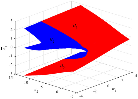
Figure 1.
Equilibrium surface (red for stability, blue for instability).
According to Appendix B, combined with the one-dimensional cubic equation with one variable, it can be seen that the catastrophe position corresponds to the critical point of the discriminant . Therefore, the condition that the catastrophe point should meet on the parameter surface is
Therefore, the catastrophe point can be obtained to form a singular point set. Figure 2 shows its projection onto the control parameter plane , which is also called a bifurcation set. The curve is a half cubic parabola, which has a cusp at , so it is called a cusp catastrophe. As the phase point moves continuously to the catastrophe point at the upper of the equilibrium surface, it will jump directly over and enter the stable equilibrium surface , since the middle of the equilibrium surface is in an unstable state.
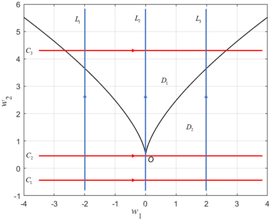
Figure 2.
The bifurcation set of system Equation (16) with the variation of control parameter .
In fact, as the control parameters change, the number and type of catastrophe are also different, that is, the system will have multiple equilibrium states under certain control parameters. As control parameter () is a fixed value, the curve L or C relevant to the other parameter () is given in Figure 2. As change along curve , the control parameter first enters area from area, and then passes back to area, it is clear that the phase point will undergo two jumps. Of course, the phase point will also experience only one or no sudden jump while changing along other curves (curve , , or , etc.). Using the corresponding curve of the parametric curve C or L on the equilibrium surface, as shown in Figure 1, the bifurcation diagram of the equilibrium point can be obtained. Then the number and the type of equilibrium points change during the catastrophe process. The bifurcation of the equilibrium point and the corresponding phase diagram are given below, as the parameters change with the series of curves C and L.
4.1. Bifurcation Analysis of the System under First-Order Wind Stress
As the corresponding second-order wind stress intensity parameter is a fixed value, is the bifurcation parameter. First, let and focus on the parameter curve shown in Figure 2. Figure 3 is the bifurcation diagram of equilibrium value of the first-order modal amplitude varying with the wind stress intensity parameter . In Figure 3, the equilibrium points in the red solid lines and indicate stable focus. The equilibrium points in the blue dashed lines and are unstable. focuses. The equilibrium points in the purple–red dashed lines and are unstable nodes. The equilibrium points in the black dashed line are saddle points. Correspondingly, the distribution of the real part, , of the eigenvalues of the derivative operator in the system at the equilibrium position is also given in Figure 4.
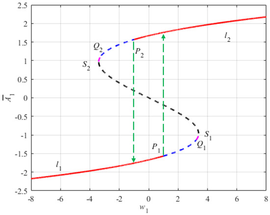
Figure 3.
Parametric curve corresponding bifurcation diagram.
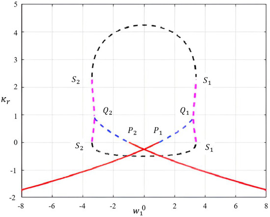
Figure 4.
The distribution of the real part, q, of the derivative operator of the equilibrium position system.
The two sudden changes occur at and on the curve, respectively. At , the equilibrium positions of the system change from one stable focus to one unstable node and one saddle point. However, the equilibrium positions at change from one stable focus, one unstable node, and one saddle point to one stable focus. With the further increase or decrease of , the unstable node becomes the unstable focus at and . It can be seen that an unstable node is experienced during the bifurcation process from the saddle point to the unstable focus. In addition, it changes from the left to the right of point , meaning it changes from a stable focus to an unstable focus. So, the system is unstable, and a supercritical Hopf bifurcation occurs at . Similarly, a subcritical Hopf bifurcation occurs as the unstable focus changes to the stable focus at .
As the bifurcation parameter increases from infinitesimal value, the phase trajectory is initially attracted to the stable branch of . As it reaches the equilibrium point at , a jump occurs. The phase trajectory jumps over the unstable branch along the green dotted line and is directly attracted to the stable branch . Conversely, as the bifurcation parameter decreases from infinity, the phase trajectory at point reaches the stable state attracted to the branch. Then it jumps over the unstable branch and is attracted to the stable branch . Therefore, in the middle area of the jump between and , there are two possible stable states of the system, which are in the black dashed part. That is, the saddle point on the unstable branch can jump to the stable upper branch or the stable lower branch, meaning the system is in a bistable state.
Figure 5 shows the corresponding bifurcation diagrams as the parameter curves and change along the bifurcation set. In Figure 5a, a sudden change occurs at with the continuous increase of . A stable point is added from the state of no equilibrium point, and then it changes to a stable focus at point B. In Figure 5b, there is no sudden change. Although the equilibrium point is always in a stable state, the type of equilibrium position switches many times as increases continuously. The stable node at the position changes to the stable focus, and the focus of position changes to a stable node. Then it changes to a stable focus at , and finally returns to a stable node at the position.
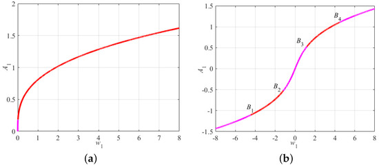
Figure 5.
Bifurcation diagram of system Equation (16) when is fixed. (a) Along parametric curve ; (b) along parametric curve .
4.2. Bifurcation Analysis of the System under Second-Order Wind Stress
As the circulation system has only second-order wind stress, the corresponding intensity parameter of the first-order wind stress is a fixed value, and is the bifurcation parameter. First, let and focus on the parameter curve in Figure 2. Figure 6 is a bifurcation diagram of the value of the first-order modal amplitude equilibrium point changing with the wind stress intensity parameter . In Figure 6, the equilibrium points in the purple solid line are stable nodes. The equilibrium points in the red solid lines and are stable focuses. However, the equilibrium points in the black dashed line are saddle points, the equilibrium points in the purple–red dashed line are unstable nodes, and the equilibrium points in the blue dashed line are unstable focuses.
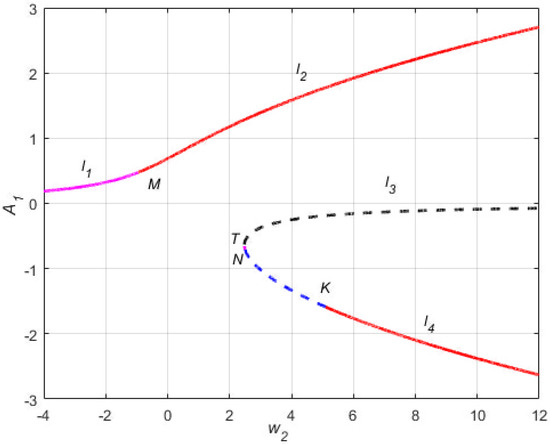
Figure 6.
The bifurcation diagram corresponding to the parameter curve .
The sudden change in the system only occurs at point T on the parameter curve . In this situation, an unstable node and a saddle point are added from the stable focus state on branch . With the further increase in the parameter , the unstable node becomes an unstable focus at N. Finally, the subcritical Hopf bifurcation occurs in the lower part of the equilibrium curve at K from an unstable focus to a stable focus, which is consistent with the sudden change along the parameter curve . At M, the transition from a stable node to a stable focus is consistent with switching the stable point as changing along the parameter curves and .
In fact, as the parameter increases, the phase trajectory of the system is always attracted to the stable node branch or the stable focus branch before point K. However, the phase trajectory of the system may be attracted to the stable focus branch or after point K. In this situation, the system has two possible stable states, i.e., in a bistable state.
Figure 7 shows the bifurcation diagrams as the parameter curves and change along the bifurcation set. For the parametric curve , the bifurcation behavior is similar to the variation along the parametric curve , as shown in Figure 7a. The stable branch is continuous in the lower branch after bifurcation, while an unstable state appears in the upper branch. From Figure 7b, it can be seen that a sudden change occurs at point O as the parameter curve changes. Then, the number and type of equilibrium points before and after point O change topologically, which is a fork bifurcation. In addition, it is clear that the bifurcation occurring along the parameter curves and is an imperfection bifurcation, and its prototype is a fork bifurcation that occurs as changes. The transition from stable nodes to stable focus also occurs at and , which is the same as the change along curve with abrupt changes at the cusp.
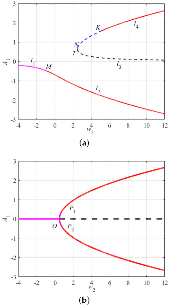
Figure 7.
Bifurcation diagram of system Equation (16) when is fixed. (a) Along parametric curve ; (b) along parametric curve .
Overall, as the value of the system parameters is distributed in the area on the corresponding bifurcation set (Figure 2), system Equation (16) has only one equilibrium state and is a stable node, , as shown in Figure 8a, or stable focus, , as shown in Figure 8b. As the wind stress intensity changes, three equilibrium states coexist in the system after passing through the catastrophe point set and entering the area, which can be divided into the following four situations: (1) unstable node, , saddle point, , and stable focus, , coexist, as shown in Figure 8c; (2) two stable focuses, and , and saddle point, , coexist, as shown in Figure 8d; (3) unstable focus, , saddle point, , and stable focus, , coexist, as shown in Figure 8e; and (4) two stable nodes, and , and saddle point, , coexist, as shown in Figure 8f.
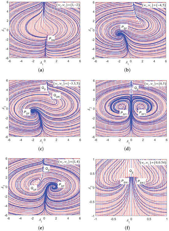
Figure 8.
The six existing states of the equilibrium point of system Equation (16). (a) Stable nodes; (b) stable focus; (c) unstable nodes, saddle points, and stable focus; (d) two stable focuses and saddle points; (e) unstable focus, saddle point, and stable focus; (f) two stable nodes and saddle points.
Although the system exhibits different types of equilibrium states depending on the wind stress intensity, there is always a stable equilibrium state present in the dynamical system, typically characterized as a stable node or stable focus. Additionally, the phase diagram reveals that, over time, the trajectory of each point tends to approach the stable equilibrium position from an unstable equilibrium position after a prolonged period of evolution.
In the study of the low-order model of the circulation system, it has been observed that the amplitude of the first two modes corresponding to the system exhibits catastrophic behavior as the wind stress intensity changes. The number and types of equilibrium states within the system undergo significant changes before and after the catastrophe. This observation further confirms that multiple equilibrium states coexist in the wind-driven ocean circulation system, and vortex motion facilitates the transition from an unstable to a stable state. As the system possesses multiple stable equilibrium states, as illustrated in Figure 8d,f, a slight disturbance can alter the final equilibrium position. In the context of the circulation system, when vortex motion is slightly perturbed by environmental factors, its state may oscillate between stable equilibrium states, potentially contributing to low-frequency oscillations observed in the atmosphere–ocean system.
5. Discussion
The results of this study provide insights into the complex dynamics of wind-driven ocean circulation systems using a Galerkin low-order model. By analyzing singular phenomena, we have demonstrated that such systems exhibit bifurcation and catastrophe behaviors under varying wind stress intensities. These findings have significant implications for understanding real-world ocean circulation structures and their influence on climate variability.
Our model highlights the intricate interplay between wind-driven forces and oceanic responses, which is essential for understanding major oceanic phenomena such as the Gulf Stream, El Niño–Southern Oscillation (ENSO), and North Atlantic Oscillation (NAO). These systems are not purely stochastic; instead, they exhibit quasi-cyclical behaviors that can be partially explained by the self-oscillation phenomena identified in our model. For instance, the Gulf Stream, a major western boundary current in the North Atlantic, plays a critical role in regulating the climate of the surrounding regions. Our findings on bifurcation and multistability align with observations that the Gulf Stream can maintain stable states, even amidst external perturbations. This stability is essential for its role in heat transport across the Atlantic Ocean, affecting weather patterns in North America and Europe.
The El Niño–Southern Oscillation (ENSO) is characterized by periodic variations in sea surface temperatures and atmospheric conditions in the equatorial Pacific. The oscillatory nature of the ENSO can be linked to the multi-equilibria states and the sensitivity of the circulation system to wind stress changes, as demonstrated in our model. The model suggests that the ENSO’s predictable patterns may result from the interaction between oceanic gyres and atmospheric winds, as discussed by McCarthy et al. (2015) and Delworth and Mann (2000) [12,13]. Similarly, the North Atlantic Oscillation (NAO) involves shifts in atmospheric pressure and wind patterns that significantly impact climate variability in the Northern Hemisphere. Our study’s insights into wind stress-induced bifurcations provide a framework for understanding how such oscillations might arise from intrinsic properties of the ocean–atmosphere system rather than being purely driven by external forces.
While our model focuses on the intrinsic dynamics of ocean circulation, it is crucial to acknowledge the role of extraterrestrial factors in shaping Earth’s climate systems. Historical and paleoclimate data suggest that factors such as Milankovitch cycles (orbital and rotational changes of Earth), solar activity variations, lunar and planetary tidal effects, and volcanic eruptions contribute to statistically significant oscillations in climate phenomena. These long-term cycles, driven by changes in Earth’s orbit and axial tilt, influence the distribution of solar energy received by Earth, thereby affecting ocean circulation patterns. Our model’s emphasis on sensitivity to parameter changes could be extended to explore how such cycles impact circulation stability and transitions. Solar radiation cycles, ranging from a few years to millennia, are known to influence Earth’s climate by altering atmospheric and oceanic circulations. The quasi-cyclical nature of ocean currents in our model may be modulated by these solar cycles, as proposed by researchers studying the ENSO and other oscillations [16].
Tidal forces exerted by the Moon and planets, along with sudden climatic shifts caused by volcanic eruptions, introduce variability in oceanic systems. The model’s ability to simulate bifurcations and transitions between stable states can help explain how such external perturbations lead to observable changes in circulation patterns. The relative stability of phenomena like the Gulf Stream, ENSO, and other large-scale ocean–atmosphere structures stems from their inherent dynamical properties. As discussed, these systems often exhibit stable and predictable behaviors due to the interplay between multiple equilibrium states and external forcing. Our model provides a theoretical foundation for understanding this stability by demonstrating how wind-driven circulation can transition between states while maintaining overall system coherence.
The methodologies presented in this study have practical applications in climate modeling and prediction. By incorporating real-world datasets, the model can be adapted to simulate specific oceanic phenomena and forecast potential changes due to varying wind stress conditions. This capability is crucial for improving weather predictions and developing strategies for climate adaptation and mitigation. In conclusion, our study advances the understanding of wind-driven ocean circulation’s complex dynamics, offering a framework to explore the multifaceted interactions between atmospheric winds, ocean currents, and climate variability. Future research should aim to integrate extraterrestrial influences and real-world data to further refine and validate the model’s predictive capabilities.
6. Conclusions
A wind-driven ocean circulation model is established based on the quasi-geostrophic vorticity equation, and the Galerkin method is used to approach the solution, resulting in a nonlinear differential dynamic system with first-order in time. Further, the dynamic behaviors of the low-order circulation model under different wind stress intensities are studied from the viewpoint of bifurcation and catastrophe theories in nonlinear dynamics, and the main conclusions can be drawn as follows.
It has been shown that there exists a cusp catastrophe in the low-order circulation system. At the catastrophe position, the state of the system changes from an unstable equilibrium to a stable equilibrium. After the cusp catastrophe, saddle nodes and unstable nodes are added to the system, and then the unstable nodes transform into unstable focuses. As wind stress intensity is constant, there is a bistable region in the circulation system as changes, and it shows hysteresis. However, as wind stress intensity parameter is constant, the fork bifurcation appears firstly in the circulation system, and then the subcritical Hopf bifurcation occurs with the increase of . In addition to the above, the results show there is a phenomenon of coexistence of multiple equilibria in the wind-driven circulation system. Interestingly, the circulation system is changed from an unstable equilibrium state to a stable equilibrium state by the vortex, and, as there are multiple stable equilibrium states, the vortex motion can be induced to oscillate by small perturbations, which could lead to a short-term climate oscillation.
Author Contributions
Conceptualization, P.F.; methodology, P.F.; software, P.F.; validation, Z.L.; formal analysis, Z.L.; investigation, P.F., S.C. and Z.L.; resources, S.C.; data curation, P.F.; writing—original draft preparation, P.F.; writing—review and editing, S.C.; visualization, S.C.; supervision, S.C.; funding acquisition, S.C. All authors have read and agreed to the published version of the manuscript.
Funding
This work is supported by the Youth program of National Natural Science Foundation of China (Grant No. 12002252), Opening project of the State Key Laboratory of Compressor Technology (No. SKL-YSJ201913), and Natural Science Basic Research Program of Shaanxi (Grant No. 2023-JC-QN-0002).
Institutional Review Board Statement
Not applicable.
Informed Consent Statement
Not applicable.
Data Availability Statement
The data used in this study are available from the corresponding author upon reasonable request.
Conflicts of Interest
The authors declare no conflicts of interest.
Appendix A. Approaching Circulation Model Using the Galerkin Method
Based on the classic quasi-geostrophic vorticity equation, the governing equation of wind-driven ocean circulation is obtained, and the Galerkin method is used to approach the solution of the circulation model. Using Equation (8), Equation (5) can be rewritten as following, namely, the quasi-geotranslocation potential equation Equation (11). Simonnet [41] proposed to expand the quasi-geostrophic vorticity equation with the eigenfunction that is suitable for the specific problem in the x and y directions, so that the computation can become easy. Considering the long-term west boundary current in the ocean, the eigenfunction or mode, that decays exponentially in the x direction and sinusoidally distributed in the y direction, is introduced in this study as Equation (12) Obviously, the eigenfunctions in Equation (12) keep orthogonal to each other, and their set can form a complete space. The solution of the quasi-geostationary potential equation Equation (11) can be projected onto the space. In addition, because of the exponential attenuation in the x direction, the eigenfunction will have nonlinear characteristics. As a projection operator, the selection of the attenuation factor s only determines its attenuation rate and does not influence the result. In this study, the attenuation factor .
Obviously, the eigenfunctions in Equation (12) keep the orthogonals to each other, and their set can form a complete space. The solution of the quasi-geostationary potential equation, Equation (11), can be projected onto the space. In addition, because of the exponential attenuation in the x direction, the eigenfunction will have nonlinear characteristics. As a projection operator, the selection of the attenuation factor, s, only determines its attenuation rate and does not influence the result. In this study, the attenuation factor .
Therefore, the expansion of the stream function can be expressed as
where represents the amplitude of the -th mode at time t. It is clear that the stream function, namely Equation (A1), satisfies the symmetry relationship, Equation (10), and the flow velocities u and v naturally satisfy this relationship.
Let the complementary function be
Using the Galerkin method, the following equations are obtained,
where is the inner product. With the Galerkin method, the unsteady term can be obtained,
Further, the convection term can be obtained,
Also, the dissipation term can be obtained,
The wind stress term should satisfy the antisymmetric relationship , which can be expressed as
where is the intensity parameter relevant to the antisymmetric wind stress. In this study, the first two modes are used. The first mode is in the form of a double-gyre, and the second mode is in the form of a four-gyre. Finally, yields,
Therefore, the solution to Equation (A3) is as follows,
where is the Kronecker symbol. As ; otherwise, it is zero. As
Then, Equation (A9) can be rewritten as follows,
Therefore, the modal amplitudes, , of the system can be obtained, and the stream function, , and the velocities u and v also can be obtained. The set of the first-order differential equations can be solved using the Runge–Kutta methods with high precision.
Appendix B. Catastrophe Behaviors of Reduced Models of Circulation System
Theoretically, the truncation of the eigenfunction used in the Galerkin procedure influences the accuracy of the solution. However, this paper aims to study the nature of ocean circulation from the viewpoint of bifurcation and catastrophe theories in nonlinear dynamics, so the low-order model can also qualitatively describe the nature of the circulation to a certain degree. This section will consider the low-order model of wind-driven circulation, i.e., the reduced positive pressure quasi-geostationary potential equation, namely Equation (11). And the influence of wind stress intensity on circulation is studied in detail.
With the first two eigenfunction or modes,
It is assumed that the wind stress intensity parameters are constant. Then, Equation (14) can be obtained as follows,
Following Equation (A10), the coefficients of the coupling terms can be given as in Equation (A13). Considering that the coefficient of horizontal momentum exchange, , is relatively large, it might as well be given as . Then the coefficient of the linear term is . For the constant term, and are variable parameters, and the coefficient is taken as .
Following the definition, the equilibrium position of system Equation (A13) satisfies . Thus the equilibrium position can be governed by the following equations,
For Equation (A14), set
So the discriminant can be obtained,
As ,
As ,
As ,
where . Therefore, as parameters and are determined, the equilibrium position can be obtained according to Equation (A15). The derivative operator of system Equation (A13) at the equilibrium position is given by the Jacobian matrix,
The eigenvalues, , of the matrix are given by the following quadratic equation,
Note that Equation (A22) is defined in the complex domain, and the type of equilibrium position depends on the eigenvalues. Since the equilibrium position is governed by the one-dimensional cubic equation, namely, Equation (A14) with two parameters , it is clear that such an equation is an extension of the governing equation for the system with a cusp catastrophe. According to the cusp catastrophe theory, Equation (A14) gives an equilibrium surface or catastrophe manifold.
Combined with the one-dimensional cubic equation with one variable, it can be seen that the catastrophe position corresponds to the critical point of the discriminant . Therefore, the condition that the catastrophe point should meet on the parameter surface is
Therefore, the catastrophe point can be obtained to form a singular point set.
References
- Ghil, M. The wind-driven ocean circulation: Applying dynamical systems theory to a climate problem. Discret. Contin. Dyn. Syst. 2017, 37, 189–228. [Google Scholar] [CrossRef]
- De Szoeke, R.A. A model of wind-and buoyancy-driven ocean circulation. J. Phys. Oceanogr. 1995, 25, 918–941. [Google Scholar] [CrossRef]
- Munk, W.H. On the wind-driven ocean circulation. J. Meteorol. 1950, 7, 80–93. [Google Scholar] [CrossRef]
- Geng, Y.; Wang, Q.; Mu, M. Effect of the Decadal Kuroshio Extension Variability on the Seasonal Changes of the Mixed-Layer Salinity Anomalies in the Kuroshio-Oyashio Confluence Region. J. Geophys. Res. Ocean. 2018, 123, 8849–8861. [Google Scholar] [CrossRef]
- Ekman, V.W. On the Influence of the Earth’s Rotation on Ocean-Currents; Almqvist & Wiksells boktryckeri, A.-B.: Uppsala, Sweden, 1905. [Google Scholar]
- Sverdrup, H.U. Wind-driven currents in a baroclinic ocean; with application to the equatorial currents of the eastern Pacific. Proc. Natl. Acad. Sci. USA 1947, 33, 318. [Google Scholar] [CrossRef] [PubMed]
- Charney, J. Generation of oceanic currents by wind. J. Mar. Res. 1955, 14, 477–498. [Google Scholar]
- Pedlosky, J. Geophysical fluid dynamics, 2nd ed.; Springer Earth Sciences: New York, NY, USA, 1987. [Google Scholar]
- Gill, A.E. Atmosphere—Ocean Dynamics; Academic Press: Cambridge, MA, USA, 1982. [Google Scholar]
- Liu, G.; Perrie, W. Sea-state-dependent wind work on the oceanic general circulation. Geophys. Res. Lett. 2013, 40, 3150–3156. [Google Scholar] [CrossRef]
- Sung, M.K.; An, S.I.; Kim, B.M.; Kug, J.S. Asymmetric impact of Atlantic multidecadal oscillation on El Niño and La Niña characteristics. Geophys. Res. Lett. 2015, 42, 4998–5004. [Google Scholar] [CrossRef]
- McCarthy, G.D.; Haigh, I.D.; Hirschi, J.J.M.; Grist, J.P.; Smeed, D.A. Ocean impact on decadal Atlantic climate variability revealed by sea-level observations. Nature 2015, 521, 508–510. [Google Scholar] [CrossRef] [PubMed]
- Delworth, T.L.; Mann, M.E. Observed and simulated multidecadal variability in the Northern Hemisphere. Clim. Dyn. 2000, 16, 661–676. [Google Scholar] [CrossRef]
- Wu, C.R.; Lin, Y.F.; Qiu, B. Impact of the Atlantic Multidecadal Oscillation on the Pacific North Equatorial Current bifurcation. Sci. Rep. 2019, 9, 1–8. [Google Scholar] [CrossRef]
- Wills, R.C.; Armour, K.C.; Battisti, D.S.; Hartmann, D.L. Ocean–atmosphere dynamical coupling fundamental to the Atlantic multidecadal oscillation. J. Clim. 2019, 32, 251–272. [Google Scholar] [CrossRef]
- Cronin, M.F.; Pelland, N.A.; Emerson, S.R.; Crawford, W.R. Estimating diffusivity from the mixed layer heat and salt balances in the N orth P acific. J. Geophys. Res. Ocean. 2015, 120, 7346–7362. [Google Scholar] [CrossRef]
- Yang, H.; Wu, L.; Shantong, S.; Zhaohui, C. Low-frequency variability of monsoon-driven circulation with application to the South China Sea. J. Phys. Oceanogr. 2015, 45, 1632–1650. [Google Scholar] [CrossRef]
- Qiu, B.; Chen, S.; Schneider, N. Dynamical links between the decadal variability of the Oyashio and Kuroshio extensions. J. Clim. 2017, 30, 9591–9605. [Google Scholar] [CrossRef]
- Wang, Q.; Pierini, S. On the role of the Kuroshio Extension bimodality in modulating the surface eddy kinetic energy seasonal variability. Geophys. Res. Lett. 2020, 47, e2019GL086308. [Google Scholar] [CrossRef]
- Liang, Z. Influence of the interaction between different low-and mid-level wind couplings and orography on the evolution of mesoscale convective systems in northwest China: A case study. Q. J. R. Meteorol. Soc. 2022, 148, 3010–3032. [Google Scholar] [CrossRef]
- Clancy, R.; Bitz, C.M.; Blanchard-Wrigglesworth, E.; McGraw, M.C.; Cavallo, S.M. A cyclone-centered perspective on the drivers of asymmetric patterns in the atmosphere and sea ice during Arctic cyclones. J. Clim. 2022, 35, 73–89. [Google Scholar] [CrossRef]
- Zuo, H.; Hasager, C.B. The impact of Aeolus winds on near-surface wind forecasts over tropical ocean and high-latitude regions. Atmos. Meas. Tech. 2023, 16, 3901–3913. [Google Scholar] [CrossRef]
- McMonigal, K.; Larson, S.; Hu, S.; Kramer, R. Historical changes in wind-driven ocean circulation can accelerate global warming. Geophys. Res. Lett. 2023, 50, e2023GL102846. [Google Scholar] [CrossRef]
- Li, H.; Hu, A.; Meehl, G.A.; Rosenbloom, N.; Strand, W.G. Impact of tropical cyclone wind forcing on the global climate in a fully coupled climate model. J. Clim. 2023, 36, 111–129. [Google Scholar] [CrossRef]
- Paldor, N.; Friedland, L. Extension of Ekman (1905) wind-driven transport theory to the β plane. Ocean Sci. 2023, 19, 93–100. [Google Scholar] [CrossRef]
- Kong, H.; Jansen, M.F. The impact of topography and eddy parameterization on the simulated Southern Ocean circulation response to changes in surface wind stress. J. Phys. Oceanogr. 2021, 51, 825–843. [Google Scholar] [CrossRef]
- Thomsen, S.; Capet, X.; Echevin, V. Competition between baroclinic instability and Ekman transport under varying buoyancy forcings in upwelling systems: An idealized analog to the Southern Ocean. J. Phys. Oceanogr. 2021, 51, 3347–3364. [Google Scholar] [CrossRef]
- Kondrashov, D.; Chekroun, M.D.; Berloff, P. Multiscale Stuart-Landau emulators: Application to wind-driven ocean gyres. Fluids 2018, 3, 21. [Google Scholar] [CrossRef]
- Sirven, J.; Février, S.; Herbaut, C. Low-frequency variability of the separated western boundary current in response to a seasonal wind stress in a 2.5-layer model with outcropping. J. Mar. Res. 2015, 73, 153–184. [Google Scholar] [CrossRef]
- Sulalitha Priyankara, K.; Balasuriya, S.; Bollt, E. Quantifying the role of folding in nonautonomous flows: The unsteady double-gyre. Int. J. Bifurc. Chaos 2017, 27, 1750156. [Google Scholar] [CrossRef]
- Jolliffe, I.T.; Cadima, J. Principal component analysis: A review and recent developments. Philos. Trans. R. Soc. A Math. Phys. Eng. Sci. 2016, 374, 20150202. [Google Scholar] [CrossRef] [PubMed]
- Golyandina, N.; Korobeynikov, A. Basic singular spectrum analysis and forecasting with R. Comput. Stat. Data Anal. 2014, 71, 934–954. [Google Scholar] [CrossRef]
- Zou, Y.; Donner, R.V.; Marwan, N.; Donges, J.F.; Kurths, J. Complex network approaches to nonlinear time series analysis. Phys. Rep. 2019, 787, 1–97. [Google Scholar] [CrossRef]
- Bryan, K.; Manabe, S.; Pacanowski, R.C. A global ocean-atmosphere climate model. Part II. The oceanic circulation. J. Phys. Oceanogr. 1975, 5, 30–46. [Google Scholar] [CrossRef][Green Version]
- Holland, W.R.; Lin, L.B. On the generation of mesoscale eddies and their contribution to the oceanicgeneral circulation. i. a preliminary numerical experiment. J. Phys. Oceanogr. 1975, 5, 642–657. [Google Scholar] [CrossRef]
- Speich, S.; Dijkstra, H.; Ghil, M. Successive bifurcations in a shallow-water model applied to the wind-driven ocean circulation. Nonlinear Process. Geophys. 1995, 2, 241–268. [Google Scholar] [CrossRef][Green Version]
- Shevchenko, I.; Berloff, P.; Guerrero-López, D.; Roman, J. On low-frequency variability of the midlatitude ocean gyres. J. Fluid Mech. 2016, 795, 423–442. [Google Scholar] [CrossRef]
- Shimokawa, S.; Matsuura, T. Chaos Excitation and Stochastic Synchronization in an Oceanic Double Gyre. Theor. Appl. Mech. Jpn. 2018, 64, 15–22. [Google Scholar]
- Primeau, F. Multiple equilibria and low-frequency variability of the wind-driven ocean circulation. J. Phys. Oceanogr. 2002, 32, 2236–2256. [Google Scholar] [CrossRef][Green Version]
- Deremble, B.; Simonnet, E.; Ghil, M. Multiple equilibria and oscillatory modes in a mid-latitude ocean-forced atmospheric model. Nonlinear Process. Geophys. 2012, 19, 479–499. [Google Scholar] [CrossRef][Green Version]
- Simonnet, E.; Ghil, M.; Ide, K.; Temam, R.; Wang, S. Low-frequency variability in shallow-water models of the wind-driven ocean circulation. Part II: Time-dependent solutions. J. Phys. Oceanogr. 2003, 33, 729–752. [Google Scholar] [CrossRef]
- Sheremet, V.; Ierley, G.; Kamenkovich, V. Eigenanalysis of the two-dimensional wind-driven ocean circulation problem. J. Mar. Res. 1997, 55, 57–92. [Google Scholar] [CrossRef]
- Dijkstra, H.A.; Katsman, C.A. Temporal variability of the wind-driven quasi-geostrophic double gyre ocean circulation: Basic bifurcation diagrams. Geophys. Astrophys. Fluid Dyn. 1997, 85, 195–232. [Google Scholar] [CrossRef]
- Ascani, F.; Firing, E.; McCreary, J.P.; Brandt, P.; Greatbatch, R.J. The deep equatorial ocean circulation in wind-forced numerical solutions. J. Phys. Oceanogr. 2015, 45, 1709–1734. [Google Scholar] [CrossRef]
- Zelik, S. Inertial manifolds and finite-dimensional reduction for dissipative PDEs. Proc. R. Soc. Edinb. Sect. A Math. 2014, 144, 1245–1327. [Google Scholar] [CrossRef]


Disclaimer/Publisher’s Note: The statements, opinions and data contained in all publications are solely those of the individual author(s) and contributor(s) and not of MDPI and/or the editor(s). MDPI and/or the editor(s) disclaim responsibility for any injury to people or property resulting from any ideas, methods, instructions or products referred to in the content. |
© 2024 by the authors. Licensee MDPI, Basel, Switzerland. This article is an open access article distributed under the terms and conditions of the Creative Commons Attribution (CC BY) license (https://creativecommons.org/licenses/by/4.0/).