Transformer-Based High-Speed Train Axle Temperature Monitoring and Alarm System for Enhanced Safety and Performance

Abstract

As the fleet of high-speed rail vehicles expands, ensuring train safety is of the utmost importance, emphasizing the critical need to enhance the precision of axel temperature warning systems. Yet, the limited availability of data on the unique features of high thermal axis temperature conditions in railway systems hinders the optimal performance of intelligent algorithms in alarm detection models. To address these challenges, this study introduces a novel dynamic principal component analysis preprocessing technique for tolerance temperature data to effectively manage missing data and outliers. Furthermore, a customized generative adversarial network is devised to generate distinct data related to high thermal axis temperature, focusing on optimizing the network’s objective functions and distinctions to bolster the efficiency and diversity of the generated data. Finally, an integrated model with an optimized transformer module is established to accurately classify alarm levels, provide a comprehensive solution to pressing train safety issues, and, in a timely manner, notify drivers and maintenance departments (DEPOs) of high-temperature warnings.

1. Introduction

Railway transportation plays a crucial role in contemporary social development [1]. In recent years, rail transit, represented by high-speed rail, has developed rapidly. As a high-quality “name card” of China, it has promoted the development and realization of the “belt and road” strategy and the “going global” strategy of China’s high-speed railway [2]. In the context of railway systems, a train is typically classified as “high-speed” if it can travel at speeds of 250 km/h (155 mph) or more on newly built tracks, or 200 km/h (124 mph) on existing tracks. This classification is essentially based on international standards set by organizations such as the International Union of Railways (UIC) and is crucial for differentiating between conventional and high-speed rail systems. The axles of high-speed trains are specifically designed to withstand these higher operational speeds, which requires enhanced durability and safety standards. How to incorporate the rapid development of big data technology to enhance the safety of train operations has become the top priority of current high-speed train development. As a crucial part of the train, the train bearing and axle box must withstand all the train’s weight. Since the train should commonly run at high speed during operation, the vibration shock due to the rough track and irregular road crossings could exhibit a remarkable impact on the bearing, so the most vulnerable parts of the train include the bearings and the axle box [3]. In general, high-speed train bearings are also the main pieces of equipment to ensure the safe operation of trains [4]. When the bearing fails and deteriorates quickly, it even endangers the safety of the train operation [5]. Therefore, effective monitoring and fault diagnosis of high-speed train bearings is an essential way to ensure the safety of train operations [6]. High-speed train axles are subject to significant mechanical and thermal stress during operation, making temperature monitoring crucial for ensuring safety and performance. While much attention has been paid to bearing temperatures, other key components, such as brake systems, also experience substantial thermal loads. In particular, brake friction pairs can be exposed to extreme temperatures, especially under conditions of brake blockage or malfunction. In such scenarios, excessive heat can be generated, which could potentially impact axle safety and performance. Therefore, comprehensive temperature monitoring, which includes the thermal behavior of both bearings and brake systems, is essential to effectively detect and mitigate risks. At present, the bearing fault diagnosis method mainly includes the diagnosis approach based on temperature data [7], the diagnostic method based on fault signal (such as acoustic signal [8,9] and vibration signal [10,11,12]), the detection and diagnosis method based on ferro-spectral analysis, the oil-based diagnosis method [13], and the diagnosis method based on oil film resistance monitoring. However, in practical application, the bearing monitoring method, which is extensively accepted in China, collects the axial temperature data through the bearing monitoring system’s sensor [14].

Since train operation monitoring and fault diagnosis technology plays a significant role in railway transportation, companies and investigators at home and abroad significantly contribute to the research of train operation monitoring and fault diagnosis technology. In the 1980s, the United States developed a bypass acoustic detection system. Through the analysis of the sound signal of the train bearings, it was combined with the infrared thermal shaft detection system to achieve the effect of detecting bearing faults in advance. SKF in Sweden proposed to use the vibration signal and shaft temperature data of bearings to monitor the working state of the axle system. The on-board fault diagnosis system was investigated at the University of Southampton, installed on a passenger train, and then utilized Perpetuum wireless sensors to measure train vibrations. The system transmits raw data and calculates measurement data to the cloud, with train number, wheel position, recording time, speed, position, direction, ambient temperature, and bearing and wheel health indexes. The operators and maintenance personnel can access real-time data through the website, monitor the health status of bearings and wheels, and determine whether failures occur [15]. Until the end of the 20th century, the railways in China began to pay attention to the detection and fault diagnosis of train bearings by utilizing the infrared axle temperature detection system and on-mounted axle temperature detection device. China Railway also adopts monitoring technology at the infrastructure management level as a diagnostic solution to improve the safety and reliability of railway operations. By deploying a large number of sensors and intelligent monitoring systems along the railway, these devices can monitor the vibration, temperature, stress, and other parameters during the operation of the train, especially the health of the axles and the status of the welding points. Although these systems are useful for fault warning, usually when the alarm is issued, the bearing damage has typically advanced to a more serious stage, still posing significant safety risks [16].

Based on the above reasons, herein, the obtained data are first methodically pre-processed, which mainly includes missing values’ treatment, outlier treatment, and normalization treatment. The axial temperature feature data with a strong thermal level is difficult to obtain, which is generated by the optimized adversary-generated network, and the objective function and discriminator in the network are optimized to enhance the effectiveness and diversity of the generated data. Finally, an optimal integration model based on the transformer module is designed to detect the alarm level. The novelty of this approach lies in the utilization of an optimized adversary-generated network to create realistic and diverse strong heat state data, overcoming the scarcity of such data. This approach ensures better generalization and robustness in the model’s performance, enhancing its ability to accurately detect alarm levels. In this way, when the abnormal increase in bearing temperature is detected, the system will immediately issue a high-temperature warning, and convey in a timely manner the warning information to the driver and relevant service departments (such as maintenance workshop, DEPO), to ensure that potential problems are quickly responded to and dealt with, and ensure the safe operation of the train and the maintenance efficiency of the equipment to the greatest extent.

2. Data Processing

The train’s advanced on-board axle temperature monitoring system ensures the accurate collection of bearing temperature data. Using the axle temperature host, the system effectively captures temperature data transmitted by sensors on the bearings and axle boxes. These critical data can then be efficiently transmitted through the network to ground storage or downloaded by personnel using the on-board temperature detection system [17]. The axle temperature data collected by the on-board axle temperature monitoring system on the train often exhibit some deficiencies. In particular, the following two issues are more common:

(1) Communication anomalies often result in partial periods of missing bearing temperature data when the train passes through tunnels or areas with weak network signals.

(2) Temperature sensor failure due to poor connections, electromagnetic interference, and other factors can lead to transient abnormalities in certain axle temperature variables that subsequently recover. These anomalies usually do not occur simultaneously in multiple sensors and therefore lead to outliers in the bearing temperature data.

The proposed methodology here is essentially based on a data-driven latent structure approach that requires normalized data during modeling. Introducing a small amount of missing axle temperature data or outliers during the modeling process could lead to noticeable modeling errors and thus affect the accuracy of fault diagnosis. As a result, appropriate data preprocessing is also performed on the acquired axle temperature data.

2.1. Missing Data Handling

In cases where there are low-density missing values in the data, common approaches include missing data removal, manual completion, regression estimation completion, or data interpolation for handling. Removing missing data can ensure data integrity but may lead to a significant waste of data resources and affect the objectivity and accuracy of the results. Manual completion is labor-intensive and not very accurate, while completing the regression estimate is complex for data with low densities of missing values. Therefore, we herein choose to use linear interpolation, a data interpolation method, as a suitable approach to deal with missing values. Common data interpolation methodologies include spline interpolation, mean imputation, multiple imputation, and maximum likelihood estimation imputation. In the present paper, linear interpolation is employed to interpolate the missing data. The main idea is that, after obtaining the historical bearing temperature data, the axial temperature data and the previous moment of the missing data are selected to estimate the missing data value. In practical applications, the reported temperature typically represents an average or maximum value, which provides a general indication of the thermal state of the axle without delving into the complexities of spatial variations. However, it is crucial to recognize the significance of temperature gradients along the axle. These gradients can cause differential expansion and contraction, leading to additional stresses and potential damage over time [18]. Studies have shown that temperature variations can indeed impact the mechanical properties and longevity of axles [19,20]. Furthermore, the temperature field along the axles is generally both time-varying and spatial-varying. The temperature field is able to vary significantly across the diameter and length of the axle, leading to gradients that may induce forces and stresses, potentially affecting the service life of the axle. These spatial and temporal variations are critical for understanding the thermal behavior of the axle but have not been accurately taken into account in the linear interpolation model used for handling missing data. Linear interpolation, while effective for simple data gaps, does not capture the complex variations in the temperature field. Future research could focus on developing more sophisticated models that account for these spatial temperature variations to enhance predictive maintenance strategies. Advanced interpolation techniques or models that consider both time-varying and spatial-varying characteristics could improve the accuracy and reliability of temperature data reconstruction, thereby providing a more comprehensive understanding of the axle’s thermal behavior and contributing to better maintenance and safety strategies.

The experimental data for this study were obtained from an on-board axle temperature monitoring system. We collected axle temperature data using 36 sensors. Data from the first 10 days were utilized to train a neural network model, and 1 day was randomly selected from eight typical locations for missing data processing. Initially, the axle temperature data collected from the temperature sensors on the train bearings were transmitted to the axle temperature monitoring system and then submitted to the ground system through network transmission. Let us assume that the train operating temperature data are represented as a data matrix X∈R^N×m, where N represents the number of samples, and m denotes the number of bearing temperature variables. In addition, the period of missing data is denoted by t∈[t₁,t₂], where t₁ represents the start time of the missing data period, and t₂ denotes the end time of the missing data period. The sampled values of bearing temperature within the period of missing data are empty. Let X be denoted as follows:

$$\mathbf{X}=\left(\begin{array}{cccc}{x}_1\left(1\right)& x_2\left(1\right)& \cdots & x_m\left(1\right)\\ x_1\left(2\right)& x_2\left(2\right)& \cdots & x_m\left(2\right)\\ ⋮& ⋮& & ⋮\\ x_1\left(N\right)& x_2\left(N\right)& \cdots & x_m\left(N\right)\end{array}\right)$$

(1)

where each row represents the axle temperature data collected at the same time for different bearing temperature variables, while each column denotes the axle temperature data collected at different times for the same bearing temperature variable. Assuming $x_i\left(k\right)$ to $x_i(k+\partial )$ for $0<\partial <N-k$ is represented as a segment of missing data. Firstly, locate the nearest data segments before and after the missing data $x_i\left(k^{\prime }\right)$ and $x_i\left(k^{″}\right)(k^{\prime }<k,k+\partial <k^{″})$.

$$x_{i,L}\left(k\right)=x\left(k^{\prime }\right)+{\displaystyle \frac{x_i\left(k^{″}\right)-x\left(k^{\prime }\right)}{k^{″}-k^{\prime }}}(k-k^{\prime })$$

(2)

where $x_{i,L}\left(k\right)$ denotes the estimated value of the missing data segment from $x_i\left(k\right)$ to $x_i(k+\partial )$, which is the result value that should be inserted into the time period with missing data. The data matrix after the interpolation of the missing data segments is denoted by X_s.

The experimental data in this article are derived from the on-board axle temperature monitoring system. During transmission, data defects may occur at points with missing data due to weak network signals when the train passes through such areas. Figure 1 shows the shaft temperature data of the vehicle after startup and before storage. A data preprocessing method based on linear interpolation is adopted to properly fill in the missing data points in the bearing temperature data. The missing values in the bearing temperature data exhibit characteristics of sparse points. Interpolation results of missing data are shown in Figure 1.

After interpolation is completed, it is also necessary to verify whether the interpolated data are significantly different from the original data. At this time, the Kolmogorov–Smirnov test (K-S test) is a commonly utilized non-parametric statistical method used to compare whether the distribution of the two sets of data is significantly different. The detailed step of the K-S one-sample test method is to exploit the actual cumulative distribution of sample sampling with the comparison of the hypothetical theoretical distribution, calculate the cumulative distribution function of the two functions, and then evaluate the maximum value D of the distance between the distribution function, and check the D-value distribution table to determine the confidence interval of the D value. If the D value is placed in the corresponding confidence interval, that is, when the maximum difference value D is in the specified numerical range, you can determine the data sample by approximately obeying or obeying the distribution of the hypothesis. However, when the difference exceeds the specified range when testing that the two data samples have a remarkable difference, the detected data samples do not meet the requirements.

In the K-S test, the primary task is to calculate the cumulative empirical distribution function of the two sets of observed data. Assuming that the samples of the datasets are expressed as (x₁, x₂, x₃,…, x_n), the cumulative distribution function is expressed as:

$$F_n\left(x\right)={\displaystyle \frac{1}{n}}{\sum }_{i=1}^i{I}_{\left[-\infty ,x\right]}\left(x_i\right)$$

(3)

where I represents the indicator function, expressed by:

$$I_{\left[-\infty ,x\right]}\left(x_i\right)=\{\begin{array}{c}1,x_i\le x;\\ 0,x_i>x;\end{array}$$

(4)

The K-S test generates a p-value for judging the distribution of the two sets of data. If the p-value is large, it means that the interpolation possesses less influence on the data distribution, and the interpolated data can be taken as consistent with the original data.

2.2. Outlier Treatment

To ensure the accuracy of the modeling and subsequent monitoring and fault diagnosis, outlier treatment is performed on the transient anomalies in certain axle temperature variable data caused by factors such as weak connections and electromagnetic interference in the collected bearing temperature data. Based on industry standards and our findings, the typical operational limit for axle-bearing temperatures in passenger trains usually ranges from 80 °C to 120 °C under normal conditions. However, temperatures could reach up to 140 °C under extreme situations without immediate risk when cooling systems and monitoring mechanisms are in place. Outliers are usually points that are significantly different from the surrounding data, so that a gradually varying temperature gradient should not be considered as outliers. This can happen by considering the continuity of the data, namely that this phenomenon should not be regarded as abnormal if the temperature value gradually rises or decreases. Smooth methods, such as moving window or sliding average, are used to identify progressive trends and avoid misidentification of temperature gradient changes as anomalies. For the anomaly detected automatically by the program, the anomaly is confirmed by manual secondary verification or a more detailed physical measurement. This can effectively prevent the true temperature change from being misjudged.

The outliers present in the data can also be considered as a type of fault. In 2014, Li et al. [21] proposed a reconstruction-based contribution method based on dynamic principal component analysis (DPCA), namely the multi-directional reconstruction contribution method. Using a continuous stirred-tank reactor (CSTR) as an example, the effectiveness of their proposed method was validated. By combining the dynamic characteristics of the axle temperature data used in this study and the long-term scale axle temperature data, the outliers belong to sparse points. Therefore, the present study also attempts to propose an effective approach for outlier reconstruction by combining DPCA and principal component search, mainly dynamic principal component search (DPCS) [22]. To this end, we commence with integrating the DPCA-based approach with variable delay expansion to extract the dynamic relationships between variables, and the matrix X_d of delayed data is obtained from X_s based on the delay time d in the following form:

$${\mathbf{X}}_d=\left(\begin{array}{c}{\mathbf{X}}_s^T(1:N-d+\mathrm{1,1}:m)\\ {\mathbf{X}}_s^T(2:N-d+\mathrm{2,1}:m)\\ {\mathbf{X}}_s^T(d:N,1:m)\end{array}\right)$$

(5)

Based on the delayed data matrix, X_d is decomposed into X_d = L+S+N as per the formula, where L,S, andNrepresent the low-rank data matrix, the sparse outlier data, and noise, respectively. By combining DPCA with DPCS via L₁-norm and convex optimization [23], the method could reconstruct the outlier data to obtain a matrix X_r of normal axle temperature data. The results of the outlier treatment of the axial temperature data used in this experiment are shown in Figure 2 and Figure 3.

In order to reduce the experimental error and improve the performance and generalization ability of the machine learning model, this paper selected the k-fold cross-validation method, and the ratio of the training set, validation set, and test set was 7:2:1, and the number of iterations was 50. The original dataset was randomly split into 3 equal-sized sub-cross validation sets, with 2 sub-cross validation sets used for model training and the remaining sub-cross validation set for model testing. The above process was repeated three times, and finally three independent model performance assessments were obtained. Using k-fold cross-validation ensured that the program had consistent performance on different subsets of the data, avoiding overfitting or underfitting.

2.3. Normalization Processing

Due to the various dimensions and magnitudes among various types of data (such as train speed, train axle temperature, and train load), the direct analysis of diverse data would affect the analysis results. Similarly, if there is a significant difference in magnitude between the data used, it would greatly affect the analysis results. To guarantee precise data analysis and reliable data modeling results, it is therefore crucial to first preprocess the raw axle temperature data by addressing missing values and outliers and then applying normalization processing. Normalization processing is able to standardize data of various types on the same scale. In the present investigation, the normalization method applied to the axle temperature data matrix after missing value handling is standard deviation normalization, which makes the data conform to a standard normal distribution with a mean of 0 and a standard deviation of 1 [24]. For the data matrix that has not been normalized, normalization processing is conducted to obtain the normalized data matrix X_p:

$$X_p={\displaystyle \frac{X_s-\mu }{\sigma }}$$

(6)

3. Screening and Regeneration of Strong Thermal Grade Characteristic Data

Due to the infrequent occurrence of strong heat states in trains, the characteristic axle temperature data for such states are relatively scarce. Using a significant amount of normal and mild heat state data alongside a limited quantity of strong heat state data could lead to poor generalization abilities of the trained model. To acquire more data regarding high-intensity heat levels in axle temperature characteristics, this chapter focuses on data generation for robust heat features and presents a methodology for generating simulated data. Based on the processed data, the results are divided into datasets that facilitate the generation of simulated data, ensuring a more balanced and comprehensive representation of high-intensity heat levels.

3.1. Selection of Axle Temperature Features

According to Chinese domestic axle temperature designs, an axle temperature raised to a level in the range of 40–60 °C is taken as mild heat, the so-called alert level; exceeding 60 °C is regarded as intense heat, classified as the alarm level [25]. However, this discrimination approach faces issues. Firstly, it involves numerous parameters such as train weight and speed, which interact and intersect with each other. Secondly, the mixture of old and new bearing types broadens the normal operating temperature range. Therefore, this study selects the temperature rise, column temperature rise difference, and vehicle temperature rise difference as the main features of the axle temperature status. By employing the same train and same car approach, the present study is capable of eliminating the influence of some crucial factors such as vehicle type, speed, and load on the axle temperature. These three indicators also serve as the main basis for axle temperature discrimination by the current HDBS-III type infrared detection equipment, validated through years of on-site experiments for their scientific validity.

The present study utilizes the Pearson correlation coefficient method for feature selection. The collected features related to axle temperature are evaluated via the Pearson correlation coefficient method to determine the correlation coefficient γ between the features and the axle temperature [26]. The range of γ is set as [−1, 1], where a higher correlation coefficient γ indicates a stronger correlation between the feature and the axle temperature. By employing this approach, irrelevant or weakly related features with the target feature are removed from the sample set. The formula for calculating the Pearson correlation coefficient can be provided as:

$$\gamma ={\displaystyle \frac{N\sum x_i{y}_i-\sum x_i\sum y_i}{\sqrt{N{\sum x_i^2-\left(\sum x_i\right)}^2}\sqrt{N{\sum y_i^2-\left(\sum y_i\right)}^2}}}$$

(7)

where N represents the number of feature samples, x_i denotes the axle temperature at the i-th instance, and y_i signifies the feature value at the i-th instance.

In this study, there exists a total of 500 data points for normal and mild heat-level axle temperature states and 200 data points for intense heat-level axle temperature states. Initially, it is necessary to expand the 200 data points for intense heat-level axle temperature states to 500 to serve as the final dataset for intense heat axle temperature states.

3.2. Generation of Intense Heat-Level Axle Temperature Feature Data

Different to the traditional generative network, the adversarial generative network consists of a generative model that captures the training set distribution and a discriminant model that tests the truth and falsehood of the data. The main task of the generative model is to receive a random noise vector as input and translate it into features similar to the real data. The initial output of the generative model may be very random, but as the number of model training epochs increases, it gradually generates more realistic samples. The training goal of the generative model is to deceive the discriminant model, making it impossible to accurately distinguish the generated samples from the real samples. The discriminant model is commonly employed to evaluate the authenticity of the input sample, and it is essentially a dichotomous model. It receives data from the generative model and real data and attempts to correctly classify them as “true” or “false” samples. The training goal of the discriminative model is to distinguish between the generated data and the real data as accurately as possible, forcing the output of the generated model to be more realistic.

This paper utilizes generative adversarial networks (GANs) for data generation. Wang et al. [27] established a fault sample generation approach with heterogeneous imbalanced monitoring data proposed by a modified GAN (the so-called mixed dual discriminator GAN, MD2GAN). As in this article, the first discriminator D is utilized to discriminate whether the generated sample is real, whereas the second discriminator F is employed to discriminate whether the generated sample is a faulty one. During the training process, the generative and discriminator models engage in adversarial learning, until the generated examples are realistic enough that the discriminator cannot effectively distinguish between real and fake examples, reaching a Nash equilibrium [28]. Finally, during sample generation, only the model generator is utilized for the generation process. The flowchart of the overall procedure is presented in Figure 4.

3.3. Discriminative Model Optimization for the Adversarial Generative Model

The reason for the pattern collapse of the GAN network is that the real data often possess a multimodal distribution, but the scoring output of the discrimination model can only be utilized to distinguish whether the input is real data or generated data, and the difference between the characteristics of the data cannot be known. This will cause the generated feature data to be concentrated at the peak of the distribution, while the data at the peak of the other distribution are almost absent. To solve this problem, in this study, an optimization layer is added to its discriminant model, so that different samples can be connected to each other, thus avoiding the pattern collapse. The schematic representation of the added optimization layer is presented in Figure 5.

For the input X∈R^N×A of the optimization layer, it is obtained after the input of the whole discriminant model goes through a fully connected layer. In the optimization layer, it first passes through a trainable 3D matrix T∈R^A×B×C to obtain M∈R^N×B×C, where N represents the total number of samples of the input discriminator. Each sample has B features, and the length of each feature is C. Taking the B feature as an example, the sum of the difference of the B feature of the current sample and the B feature of all samples should be appropriately calculated. The formula is presented in Equation (6). At present, the difference between the two samples is evaluated via the paradigm distance formula L1:

$$\begin{gathered} c_b(x_i,x_j)=\mathit{exp}(-‖M_{i,b}-{M_{j,b}‖}_{L1}) \\ o(x_i{)}_b={\sum }_{j=1}^N{c}_b(x_i,x_j) \end{gathered}$$

(8)

Each feature of each sample is calculated according to the above expression, and the sum of distance differences between the i-th sample and the corresponding features of the other sample is taken as the output o(x_i) of the sample after the optimization layer, whose expression is illustrated in Equation (7):

$$o\left(x_i\right)=\left[o(x_i{)}_1,o(x_i{)}_2,\dots ,o(x_i{)}_B\right]$$

(9)

At this time, the output of the optimization layer for all samples is described by Y∈R^N×B, whose expression is given by Equation (8):

$$Y=\left[o\left(x_1\right),o\left(x_2\right),\dots ,o\left(x_N\right)\right]$$

(10)

Finally, the optimization layer of output and input after combining columns as the input is included, and the optimization layer of the output and the basic output of the generated network are added. Thereafter, each sample will receive a score to judge the input data after iteration according to the target function of the model parameters.

3.4. Generation of the Strong Thermal Signature Data

One of the aims of this study is to generate 500 intense heat state feature data based on the existing 200 intense heat state feature data. During the model training process, the shapes of the input noise for the generator are (Batch and Feature), where batch represents the batch of input noise to the generator model, and feature denotes the dimension of the noise shape. At this stage, the Batch value is 40 and the Feature value is 16. During parameter iteration, the detector parameters are fixed when the generator model parameters are updated, and, similarly, the generator parameters are frozen when the detector model parameters are updated [29]. Both models utilize the Adam optimizer with beta parameters (0.5, 0.999). The training phase includes a total of 2000 iterations, where the model storage is performed every 200 iterations. Upon the completion of model training, generating intense heat axle temperature state features only requires the use of the generator model. At this stage, 10,000 noise features of length 16 are input for generation, and 500 generated feature data are randomly selected according to the criteria of concern.

For the three features of temperature rise, column temperature rise difference, and vehicle temperature rise difference, the temperature rise value must be greater than both the temperature rise differences of the column and the vehicle. This limitation is very important. To ensure that the generated intense heat-level feature data demonstrate diversity, the Euclidean distance between the samples generated by the generator G must exceed 2, which ensures great dissimilarity between the samples. In addition, a random selection of generated and authentic intense heat samples can be performed, followed by dimensionality reduction to two dimensions using the T-SNE method, to facilitate subsequent training of the alarm system model [30]. Subsequently, the reduced dimensional data for real and generated data are extracted separately and visualized, as depicted in Figure 5.

The left shows the feature data generated using the adversarial generative network before optimization, and the left demonstrates the optimized feature data on the right. In fact, the principle of T-SNE is a probabilistic-based approach to measure the similarity between high dimensional data points and try to preserve these similarities in low dimensional space. Therefore, the results of the feature data of the real strong thermal axis temperature state in the two graphs after employing the T-SNE algorithm are not identical, but this does not affect the distinction between the distribution of the strong thermal feature data generated before and after optimization and the real feature distribution. After comparison, the two graphs show that the data distribution of the optimized adversarial generated network is closer to the distribution of real data compared with the unoptimized generated data.

In the optimized adversarial generated network according to the definition of adversarial generative network, in the process of network training, the parameters of the discriminative model are iterated by comparing the real feature data and the feature data generated by the generative model through the difference output after the discriminative model. With the increase in the iterations of the adversarial generation network, the difference between the two will gradually decrease, making it impossible for the discriminant model to judge whether the data are generated or real. Based on this idea, the quality of the generated data is judged by the comparison of the difference between the output of the generated feature data and the real data input. The experimental results show that the absolute difference of the output before optimization is 0.39 and the optimized output is 0.25, indicating that the quality of the strong thermal axis temperature state feature data generated after optimization is higher.

Figure 6 indicates on the right side that the strong thermal-level axial temperature data can generate the characteristic data, and the real characteristic data distribution is roughly the same. After dimension reduction in many real feature data distributions, denser peaks exhibit more generated feature data. In addition, these data indicate that it is easier to identify the strong thermal-level of axial temperature data, generated in the peak connection and the rest of the axial temperature state of the strong thermal characteristic data. The addition of these axial temperature data could assist the alarm model to better distinguish between the two states of strong heat and micro heat.

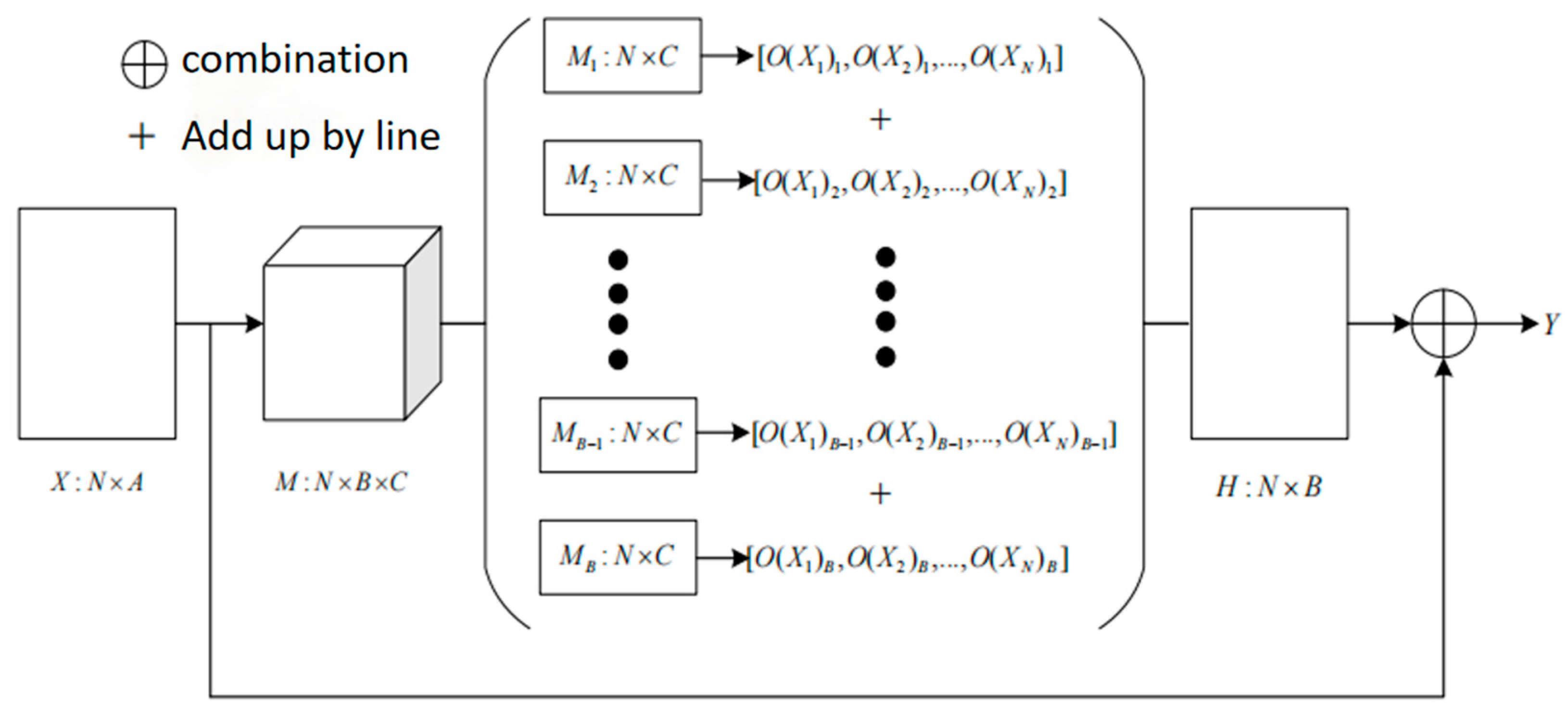
4. Intelligent Algorithm Model for Determination of the Axle Temperature Alarm Level

4.1. Training the Axle Temperature Alarm-Level Discrimination Model

This paper adopts a discriminative approach that determines the relationship weights between sequences through the collective action of multiple attention mechanism layers and finally integrates the results of each attention mechanism layer to obtain the final information [31]. In terms of training the alarm level discrimination network, the whole discrimination model consists of a transformer module and an output layer. To construct the transformer, the most crucial aspect of the whole model is the selection of the number of layers of the attention mechanism and the number of neurons in the hidden layer. Since the number of input features is small, only one transformer module is utilized to extract information from the input sequence samples. The components of a transformer are presented in

Table 1. Test set accuracy and loss values.

The Fold Times k	Loss Value/%	Precision/%
1	4.63	98.62
2	9.52	97.88
3	7.36	98.03
Average	7.17	98.17

.

As shown in

Table 2. Structure of the transformer model.

Layer Type	Output Type	Parameter Value
Embedding	(Batch, 3, 3)	256
Multi-head attention	(Batch, 3, 64)	16,640
Add	(Batch, 3, 64)	0
Layer norm	(Batch, 3, 64)	0
FFN	(Batch, 3, 64)	33,088
Add	(Batch, 3, 64)	0
Layer norm	(Batch, 3, 64)	0
Output	(Batch, 3, 4)	260

, is a component of a Transformer. For the basic axle temperature alarm-level determination model, since the total number of parameters in the model is very small, with only fifty thousand learnable parameters, the excessive number of neurons in the hidden layer could lead to overfitting of the discrimination model [31]. Therefore, the number of neurons in the hidden layer is herein set as 64. Additionally, to ensure the effectiveness of the multi-head attention mechanism layer, the dimensions of the Q, K, and V vectors for each attention mechanism cannot be too low. Simultaneously, the number of neurons in the hidden layer must be divisible by the number of attention layers in the multi-head attention mechanism layer. Therefore, the number of attention layers in the multi-head attention mechanism layer is set to 2, which means that the dimensions of the Q, K, and V vectors for each attention mechanism are 32.

The alarm-level discrimination model benefits from two sets of inputs: the sequence features of the input sequence and the position vector of the detection station. The sequence features of the input sequence, denoted by X in the model training phase, have the form (Batch, Seq, Feature), where the first, second, and third dimensions represent the data batch processed simultaneously, the number of detection stations considered, and the selected number of features, respectively. In the model training stage, Batch in X can be selected based on the computer performance, while Seq and Feature sizes are fixed at 3. For instance, consider the i-th sample X_i within a sequence of samples X as follows: X_i = (x1, x2, x3), where X_i represents a vector of axle temperature features detected by the detection station, with corresponding values (f1, f2, f3). Specifically, the arrangement of axle temperature feature data obtained by the i-th detection station in order are temperature rise, column temperature rise difference, and vehicle temperature rise difference. For the sequence length in the alarm rule Seq less than 3 optimized timing sample data, the missing part of the corresponding vector is [−2, −2, −2]. For example, for a training sample, only the first detection station of axial temperature characteristic information, then for the second and three detection stations corresponding to the vector [−2, −2,−2]. For another discriminant model, the input position vector is denoted by P, which is a fixed vector [1, 2, 3], so the input formula of the multi-head attention mechanism layer is given by:

$$E=drop(W_{xe}X+W_{pe}P)$$

(11)

In Formula (9), W_xe is the timing of the input feature vector by embedding layer mapping to hidden layer neurons a number of the weight matrix, W_pe is used for position information mapping weight matrix, eventually both and through the dropout layer containing the output of position information and characteristic information of E, after the long attention mechanism layer and the residual connection for the first time.

$$MultiHead(Q,K,V)=Concat(hea{d}_1,\dots ,hea{d}_h)W_o$$

(12)

$$hea{d}_i=Attention(Q{W}_i^Q,K{W}_i^K,V{W}_i^V)$$

(13)

$$Attention(Q,K,V)=soft\mathit{max}(Q{K}^T/\sqrt{d_k})V$$

(14)

$$A=E+Norm\left(MultiHead\right(Q,K,V\left)\right)$$

(15)

The first formula above represents the output of the multi-head attention mechanism layer composed of the output of multiple attention mechanism layers. W_o is the output transformation matrix. h represents the number of attention mechanism layers contained in the multi-head attention mechanism layer. The output of each header can be expressed by the second formula, where W_i^Q, W_i^K, and W_i^V are the query, key, and value transformation matrix of the i-th head. Q, K, and V represent the query vector, the key vector, and the value vector, respectively. In this study, since the self-attention mechanism is used, the values of Q, K, and V are all from E. The output of the attention mechanism layer is calculated as shown in the third formula, where d_k is the dimensional size of the vector Q. The final output is shown in the fourth formula, where the residual connection and norm layer normalization are used to improve the generalization ability of the model.

Then, there is a normalization layer, which is composed of two fully connected layers, and the final output result is obtained through the second residual connection.

4.2. Axle Temperature Alarm-Level Discrimination

For the prediction stage, the input is the same as the training stage, but, at this point, the Batch value of X is fixed to 1, Feature to 3, and Seq can be of any length. Figure 7 illustrates the input scenario during the model’s decision-making process.

The entire section in Figure 7 represents the sequence of input features X to the model during the prediction process. Taking a time window as an example, the width of the time window corresponds to the sequence length Seq in the training process of the discrimination model, while the height represents the selected number of features, the so-called Feature. As the time window continuously slides, the single-time feature samples obtained by detection station 3 will integrate the axle temperature feature information obtained by the previous two detection stations. In the case of a train start-up, when the sequence length Seq is less than 3, only the feature data obtained by the current detection station are considered. In the final validation process of this study, the accuracy of detection is considered based on various sequence lengths of feature data input to the discrimination model. The values of the input sequence length range from 1 to 10, which ensures the efficiency of the model in predicting alarm levels.

4.3. Optimization of the Axle Temperature Alarm-Level AdamW-Based Discriminator Model

In the former process of determination of the axle temperature alarm level, only the prediction and evaluation of axle temperature alarm levels are conducted. At this stage, the model acquires the probability values associated with various levels of alarm grades through three main steps. Firstly, useful information is extracted through the transformer model, and after passing through a fully connected layer, the output 0 is obtained. The shape of 0 is (Batch, 3, 4). After that, the maximum sequence corresponding to the predictions from the second dimension 0 is extracted (from right to left, where the rightmost is the first dimension), resulting in the prediction results in Pr with a shape of (Batch, 4). Finally, Pr is normalized along the first dimension to obtain the probability values of the model’s judgments at various alarm levels of the input data. In this step, the indicators used for model parameter iteration include the model-predicted probabilities of axle temperature alarm levels and the corresponding cross-entropy loss function values for the real alarm levels.

To optimize the existing loss function, the value of the cross-entropy loss function is therefore included between the predicted probability of axle temperature states based on the detection station judgment and the true axle temperature state labels. Consequently, for the output of the transformer module in the model, two distinct fully connected layers are required to extract the probabilities of each axle temperature alarm level and the probabilities of the axle temperature states for the three detection stations, as shown in Figure 8.

Due to the sequential nature of detection at detection stations, the input feature vector of the current detection station to the model should only interact with the features obtained from previous detection stations through the attention mechanism (i.e., interaction with the features obtained from subsequent detection stations should not occur). It is hence crucial to optimize the multi-head attention mechanism in the alarm-level discrimination by incorporating the masked multi-head attention mechanism. The loss function at this point can be calculated through the following formula:

$$L={\displaystyle \sum _{n=1}^N}-\log (y_i^{(n)})+\omega {\displaystyle \sum _{n=1}^N}-{\lambda }_1\log (p_1^{(n)})-{\lambda }_2\log (p_2^{(n)})-{\lambda }_3\log (p_3^{(n)})$$

(16)

In Equation (6), the first term on the right-hand side signifies the loss caused by the prediction of axle temperature alarm levels for the current batch of feature data, whereas the remaining terms denote the loss caused by the axle temperature states of the three detection stations. In addition, ω represents the proportion of the axle temperature state prediction to the total loss. The factors ${\lambda }_1$, ${\lambda }_2$, and ${\lambda }_3$ denote the weights of the entire axle temperature state loss pertinent to the first, second, and third detection stations, respectively, while $p_1^{(n)}$, $p_2^{(n)}$, and $p_3^{(n)}$ represent the model output probabilities associated with the correct axle temperature states for the first, second, and third detections. It should be herein emphasized that, in the case of a train just starting up or restarting (when the sequence length is less than 3 and the missing parts are replaced with vectors all set to −2), the corresponding loss should be removed.

The iteration curves for the training and validation sets at ${\lambda }_1$, ${\lambda }_2$, and ${\lambda }_3$ (corresponding to 1, 3, and 9) are presented in Figure 9.

The plotted results in Figure 9 reveal that, when the number of iterations reaches 4000, the validation loss and training loss become almost stabilized. At this stage, the accuracy of the training set reaches 87.8% and the accuracy of the validation set touches 90.9%. Subsequently, using the remaining 10% of “normal”- and “mild”-level feature data, along with all the real “intense”-level feature data, a test set sample is constructed via the same methodology and input in the trained model. The obtained results are indicative of the accuracy of the test set being 86.9% compared with designing an axle temperature alarm system based solely on the axle temperature states detected at each monitoring station, which yields an alarm accuracy of 76.8%, exhibiting an accuracy increase of 13.2%. In addition to the AdamW optimizer, incorporating momentum-based optimizers like Nesterov accelerated gradient (NAG) or using optimization algorithms such as RMSprop or AdaGrad might yield faster convergence. It should be emphasized here that gradient clipping could prevent exploding gradients, enhancing stability during training. Furthermore, for the trained model at this stage, predicting the axle temperature alarm level at time T only requires inputting the current detected axle temperature feature data. The model automatically combines previous axle temperature feature data to provide an alarm level at time T.

5. Conclusions and Perspectives

This study conducted data preprocessing on the collected data to effectively utilize temperature rise features, along with column and vehicle temperature rise difference features for axle temperature alarms. It also integrated the existing method of axle temperature alarm-level discrimination based on these features. Addressing the challenges posed by the infrequent occurrence and difficulty in obtaining data related to intense heat axle temperature states in trains, which results in a scarcity of intense heat axle temperature feature data and hinders the training of a generalized axle temperature alarm-level discrimination model, this study developed an optimized generative adversarial network (GAN) for simulating the generation of limited intense heat feature data. Subsequently, the generated intense heat feature data were integrated with existing intense heat, mild heat, and normal feature data to generate sequence feature data for the warning-level discrimination model. Finally, using a transformer block, the alarm-level discrimination model enhanced the loss function by introducing cross-entropy loss based on the axle temperature states. The present study aims to provide comprehensive training, validation, prediction, and in-depth analysis on hyperparameter design, loss function optimization, and model integration.

References

1. Lukianenko, N. Epistemological research problems of rail transport as a social institution. Transp. Res. Proceed. 2022, 63, 1826–1833. [Google Scholar] [CrossRef]
2. Chen, X. Cross-cultural communication in the belt and road strategy. Front. Soc. Sci. Technol. 2021, 3, 48–56. [Google Scholar] [CrossRef]
3. Tang, W.C.; Wang, M.J.; Chen, G.D. Analysis on temperature distribution of failure axle box bearings of high speed train. J. China Railw. Soc. 2016, 38, 50–56. [Google Scholar] [CrossRef]
4. Randall, R.B. Vibration-Based Condition Monitoring: Industrial, Aerospace and Automotive Applications; John Wiley & Sons: Hoboken, NJ, USA, 2011; pp. 13–20. [Google Scholar]
5. Yi, C.; Lin, J.; Zhang, W.; Ding, J. Faults diagnostics of railway axle bearings based on IMF’s confidence index algorithm for ensemble EMD. Sensors 2015, 15, 10991–11011. [Google Scholar] [CrossRef]
6. Henao, H.; Kia, S.H.; Capolino, G.-A. Torsional-vibration assessment and gear-fault diagnosis in railway traction system. IEEE Trans. Ind. Electron. 2011, 58, 1707–1717. [Google Scholar] [CrossRef]
7. Tchakoua, P.; Wamkeue, R.; Ouhrouche, M.; Slaoui-Hasnaoui, F.; Tameghe, T.A.; Ekemb, G. Wind turbine condition monitoring: State-of-the-art review, new trends, and future challenges. Energies 2014, 7, 2595–2630. [Google Scholar] [CrossRef]
8. Kilundu, B.; Chiementin, X.; Duez, J.; Mba, D. Cyclostationarity of Acoustic Emissions (AE) for monitoring bearing defects. Mech. Syst. Signal Process. 2011, 25, 2061–2072. [Google Scholar] [CrossRef]
9. Eftekharnejad, B.; Carrasco, M.R.; Charnley, B.; Mba, D. The application of spectral kurtosis on acoustic emission and vibrations from a defective bearing. Mech. Syst. Signal Process. 2011, 25, 266–284. [Google Scholar] [CrossRef]
10. Sun, H.; Zi, Y.; He, Z. Wind turbine fault detection using multiwavelet denoising with the data-driven block threshold. Appl. Acoust. 2014, 77, 122–129. [Google Scholar] [CrossRef]
11. Ming, A.B.; Zhang, W.; Qin, Z.Y.; Chu, F.L. Envelope calculation of the multi-component signal and its application to the deterministic component cancellation in bearing fault diagnosis. Mech. Syst. Signal Process. 2015, 50, 70–100. [Google Scholar] [CrossRef]
12. Zimroz, R.; Bartelmus, W.; Barszcz, T.; Urbanek, J. Diagnostics of bearings in presence of strong operating conditions non-stationarity—A procedure of load-dependent features processing with application to wind turbine bearings. Mech. Syst. Signal Process. 2014, 46, 16–27. [Google Scholar] [CrossRef]
13. Kharche, P.P.; Kshirsagar, S.V. Review of fault detection in rolling element bearing. Int. J. Innov. Res. Adv. Eng. 2014, 1, 169–174. [Google Scholar]
14. Liu, C.; Wang, F. A review of current condition monitoring and fault diagnosis methods for low-speed and heavy-load slewing bearings. In Proceedings of the 2017 9th International Conference on Modelling, Identification and Control (ICMIC), Kunming, China, 10–12 July 2017; pp. 104–109. [Google Scholar]
15. Corni, I.; Symonds, N.; Wood, R.J.K.; Wasenczuk, A.; Vincent, D. Real-time on-board condition monitoring of train axle bearings. In Proceedings of the Stephenson Conference, London, UK, 21–23 April 2015; p. 14. [Google Scholar]
16. Jayaswal, P.; Wadhwani, A.K.; Mulchandani, K.B. Machine fault signature analysis. Int. J. Rotat. Mach. 2008, 2008, 583982. [Google Scholar] [CrossRef]
17. Singh, K. Smart Components: Creating a Competitive Edge through Smart Connected Drive Train on Mining Machines. Master’s Thesis, KTH, School of Industrial Engineering and Management (ITM), Stockholm, Sweden, 2021. [Google Scholar]
18. Xu, Q.; Sun, S.; Xu, Y.; Hu, C.; Chen, W.; Xu, L. Influence of temperature gradient of slab track on the dynamic responses of the train-CRTS III slab track on subgrade nonlinear coupled system. Sci. Rep. 2022, 12, 14638. [Google Scholar] [CrossRef] [PubMed]
19. Yang, L.; Xu, P.; Yang, C.; Guo, W.; Yao, S. High-temperature mechanical properties and microstructure of 2.5 DC/C–SiC composites applied for the brake disc of high-speed train. J. Eur. Ceram. Soc. 2024, 44, 116683. [Google Scholar] [CrossRef]
20. Kebede, Y.B.; Yang, M.-D.; Huang, C.-W. Real-time pavement temperature prediction through ensemble machine learning. Eng. Appl. Artif. Intell. 2024, 135, 108870. [Google Scholar] [CrossRef]
21. Li, G.; Qin, S.J.; Chai, T. Multi-directional reconstruction based contributions for root-cause diagnosis of dynamic processes. In Proceedings of the 2014 American Control Conference, Portland, OR, USA, 4–6 June 2014; pp. 3500–3505. [Google Scholar]
22. Song, Y.; Ma, Q.; Zhang, T.; Li, F.; Yu, Y. Research on fault diagnosis strategy of air-conditioning systems based on DPCA and machine learning. Processes 2023, 11, 1192. [Google Scholar] [CrossRef]
23. Candès, E.J.; Li, X.; Ma, Y.; Wright, J. Robust principal component analysis? J. ACM 2011, 58, 1–37. [Google Scholar] [CrossRef]
24. Li, Z.; He, Q. Prediction of railcar remaining useful life by multiple data source fusion. IEEE Trans. Intell. Transp. Syst. 2015, 16, 2226–2235. [Google Scholar] [CrossRef]
25. Yan, G.; Yu, C.; Bai, Y. A new hybrid ensemble deep learning model for train axle temperature short term forecasting. Machines 2021, 9, 312. [Google Scholar] [CrossRef]
26. Pan, Z.; Xu, D.; Zhang, Y.; Wang, M.; Wang, Z.; Yu, J.; Zhang, G. New energy transmission line fault location method based on Pearson correlation coefficient. In Proceedings of the 2nd International Conference on Smart Energy, Fenghuang, China, 29–30 July 2024; p. 012007. [Google Scholar]
27. Wang, C.; Liu, J.; Zio, E. A modified generative adversarial network for fault diagnosis in high-speed train components with imbalanced and heterogeneous monitoring data. J. Dyn. Monit. Diagn. 2022, 1, 84–92. [Google Scholar] [CrossRef]
28. Jabbar, A.; Li, X.; Omar, B. A survey on generative adversarial networks: Variants, applications, and training. ACM Comput. Surv. (CSUR) 2021, 54, 1–49. [Google Scholar] [CrossRef]
29. Yildirim, M.; Sun, X.A.; Gebraeel, N.Z. Sensor-driven condition-based generator maintenance scheduling—Part I: Maintenance problem. IEEE Trans. Power Syst. 2016, 31, 4253–4262. [Google Scholar] [CrossRef]
30. Matetić, I.; Štajduhar, I.; Wolf, I.; Ljubic, S. A review of data-driven approaches and techniques for fault detection and diagnosis in HVAC systems. Sensors 2022, 23, 1. [Google Scholar] [CrossRef]
31. Lv, H.; Chen, J.; Pan, T.; Zhang, T.; Feng, Y.; Liu, S. Attention mechanism in intelligent fault diagnosis of machinery: A review of technique and application. Measurement 2022, 199, 111594. [Google Scholar] [CrossRef]
Figure 1. The time-varying temperature of various axles in 2 data samples: (a) axle 1; (b) axle 2; (c) axle 3; (d) axle 4; (e) axle 5; (f) axle 6; (g) axle 7; (h) axle 8.
Applsci 14 08643 g001
Figure 2. Before data processing of the outlier axle temperature.
Applsci 14 08643 g002
Figure 3. After data processing of the outlier axle temperature.
Applsci 14 08643 g003
Figure 4. Flowchart of training the adversarial generative networks.
Applsci 14 08643 g004
Figure 5. Schematic representation of the optimization layer for the discriminant model.
Applsci 14 08643 g005
Figure 6. Comparison of data visualization of strong thermal features generated before and after optimization.
Applsci 14 08643 g006
Figure 7. Input to the prediction stage model.
Applsci 14 08643 g007
Figure 8. Input to the new prediction stage model.
Applsci 14 08643 g008
Figure 9. Variations of λ1, λ2, and λ3 during iteration process.
Applsci 14 08643 g009