Abstract
Soil consolidation, particularly in fine-grained soils like clay, is crucial in predicting settlement and ensuring the stability of structures. Additionally, the compressibility of fine-grained soils is of critical importance not only in civil engineering but also in various other fields of study. The compression index (Cc), derived from soil properties such as the liquid limit (LL), plastic limit (PL), plasticity index (PI), water content (w), initial void ratio (e0), and specific gravity (Gs), plays a vital role in understanding soil behavior. This study employs machine learning algorithms—the random forest regressor (RFR), gradient boosting regressor (GBR), and AdaBoost regressor (ABR)—to predict the Cc values based on a dataset comprising 915 samples. The dataset includes LL, PL, W, PI, Gs, and e0 as the inputs, with Cc as the output parameter. The algorithms are trained and evaluated using metrics such as the coefficient of determination (R2), mean absolute error (MAE), mean squared error (MSE), and root mean squared error (RMSE). Hyperparameter optimization is performed to enhance the model performance. The best-performing model, the GBR model, achieves a training R2 of 0.925 and a testing R2 of 0.930 with the input combination [w, PL, LL, PI, e0, Gs]. The RFR model follows closely, with a training R2 of 0.970 and a testing R2 of 0.926 using the same input combination. The ABR model records a training R2 of 0.847 and a testing R2 of 0.921 under similar conditions. These results indicate superior predictive accuracy compared to previous studies using traditional statistical and machine learning methods. Machine learning algorithms, specifically the gradient boosting regressor and random forest regressor, demonstrate substantial potential in predicting the Cc value for fine-grained soils based on multiple soil parameters. This study involves leveraging the efficiency and effectiveness of these algorithms in geotechnical engineering applications, offering a promising alternative to traditional oedometer testing methods. Accurately predicting the compression index can significantly aid in the assessment of soil settlement and the design of stable foundations, thereby reducing the time and costs associated with laboratory testing.
1. Introduction
The compressibility of fine-grained soils is critically important across multiple fields of study. In civil engineering, the compression characteristics of fine-grained soils under a load affects the stability of structures such as buildings and roads; therefore, engineers must carefully account for this property to prevent issues like differential settlement and structural damage. In addition, in environmental engineering, understanding soil’s low permeability due to its compressibility helps in designing effective barriers against contaminant migration in groundwater [1,2,3]. This knowledge is vital for safeguarding water resources and managing hazardous waste disposal sites. Moreover, soil compressibility influences soil fertility, water retention, and drainage, directly impacting crop growth in agriculture [4,5,6]. Farmers adapt their irrigation and drainage practices to optimize agricultural productivity and prevent soil erosion. Additionally, in soil science, soil’s compressibility is integral to soil classification systems and understanding soil behavior under different conditions. This knowledge supports land use planning, environmental assessments, and sustainable soil management practices. Overall, a comprehensive understanding of the compressibility of soils enhances our ability to address challenges in infrastructure stability, environmental protection, agricultural productivity, and soil conservation across various disciplines.
Consolidation is a process applied to fine-grained soils. It involves slowly compressing the water in these soils under a load and removing it through drainage. Fine-grained soils, particularly clay, exhibit unique characteristics such as high compressibility, which play crucial roles across various disciplines. In the engineering field, this process increases the load carrying ability of the ground and minimizes long-term settlement, significantly affecting structural strength. Consolidation is particularly critical in fine-grained soils like clay because they react more slowly to the movement of water under a load. The compressibility of soils is quantified using the compression index (Cc), an important measurement for understanding settlement behavior. The compression index indicates the logarithmic amount of settlement per unit load increment and is typically determined in the laboratory through consolidation tests. This parameter is crucial in engineering applications for predicting soil behavior and developing appropriate foundation designs [7].
In geotechnical engineering, the evaluation and prediction of soil behavior under various loading conditions are critical for the stability and longevity of civil engineering structures. Key soil properties influencing such behavior include the liquid limit (LL), plastic limit (PL), water content (w), plasticity index (PI), specific gravity (Gs), and initial void ratio (e0), all of which are integral to calculating the compression index of soils. The liquid limit (LL) denotes the water content level at which the soil transitions from liquid to plastic, while the plastic limit (PL) marks the shift from plastic to semi-solid, essential for characterizing soil plasticity [8]. Water content directly impacts soil’s consistency and compressibility and is pivotal in soil behavior analysis [9]. The plasticity index, derived from the difference between the LL and PL, provides a comprehensive measure of soil plasticity, influencing its mechanical properties [7]. The initial void ratio (e0), expressing the volumetric relationship between soil voids and solids, significantly determines the soil compression and settlement potential under a load (Head, 1980). Furthermore, specific gravity (Gs), evaluating the particle density of soil relative to water, is crucial for understanding soil compressibility and stress behavior [10]. These parameters collectively contribute to determining the Cc value, a critical metric for predicting soil compression under loading [11]. The interrelation and influence of these soil properties on the Cc value are fundamental in geotechnical investigations and form the basis of effective soil behavior modeling and predictive analysis in civil engineering. From the 1950s to the present, research on consolidation processes has prompted the development of several important equations. These equations are critical in geotechnical engineering for understanding and predicting the compression behavior of fine-grained soils. These mathematical models are utilized to forecast how soils will respond under a load, offering precise settlement predictions for engineering applications. Table 1 summarizes the evolution of these equations over time.

Table 1.
Evolution of the prediction equations for the compression index (Cc) over history.
The use of computational intelligence methods, such as artificial neural networks (ANNs), is extensively combined with traditional statistical techniques like regressions [28,29,30]. These techniques have been widely employed in various geotechnical problems, such as estimating the Cc parameter [31,32,33]. However, different solution approaches for these problems yield varying results. The goal is to identify the algorithms that yield the most accurate predictions. Deep learning and machine learning algorithms, which are sub-branches of artificial intelligence, offer predictive equations.
An area of data science and artificial intelligence called machine learning (ML) makes use of algorithms and statistical models to facilitate the automated acquisition of knowledge by computers via experience so they can perform certain tasks without being explicitly programmed. This process provides the ability to recognize patterns from data and make decisions, allowing machines to solve complex problems and make predictions [34]. In fields such as geotechnical engineering and consolidation, machine learning methods are increasingly used to more accurately predict soil properties and behavior, model soil compaction and consolidation, and optimize engineering designs. These techniques can improve risk assessments, streamline construction processes, and increase the reliability of engineering solutions [35].
Studies have been published in the literature that accurately predict the compression index using various machine learning methods. Utilizing an artificial neural network (ANN), a machine learning technique, researchers predicted the compression index using a dataset that included parameters like w, LL, PI, and Gs [27]. Benbouras et al. [36] used ANN models, genetic programming, and multiple regression analysis to estimate the compression index on a dataset that contained LL, w, FCs (fine contents), Ph (wet density), PI, e0, and soil types. In addition, Tsang et al. [37] employed machine learning techniques like extreme gradient boosting and random forest models on a dataset comprising e0, w, LL, PI, and Gs to predict the compression index. Also, Chia et al. [38] utilized random forest (RF) and gradient boosting tree (GBT), tree-based machine learning techniques, with input parameters including LL, e0, PL, and moisture content (MC) to determine the value of Cc. Lastly, Kim et al. [39] predicted the compression index using an ANN model, a form of deep learning, on a dataset containing w, PI, LL, and the compression index (Cc).
Artificial intelligence methods are increasingly being used in various soil and rock analyses in geotechnical engineering, yielding successful results. Baghbani et al. [40] reported that artificial neural networks (ANNs) are the most widely used method and emphasized that artificial intelligence methods successfully predict complex relationships in geotechnical engineering, particularly in areas such as frozen soils, rock mechanics, and slope stability. Qader et al. [41] analyzed the geotechnical properties of soils in Erbil using geographic information systems (GISs) and artificial neural networks (ANNs), successfully estimating parameters such as SPT-N and the bearing capacity of soils, which were predominantly in the silty clay (CL) class. Their study demonstrated that these techniques provide valuable information for soil analysis. Additionally, Jolfaei and Troncone [42] examined the breakout dimensions caused by drilling in a rock environment using the finite element method. They then developed a model that estimated the breakout dimensions using artificial neural networks, finding that the internal friction angle has the greatest influence on the breakout dimensions.
The primary aim of this work is to conduct a comparative evaluation of various machine learning algorithms for predicting the compression index (Cc) of soils, using soil properties such as LL, PL, w, PI, Gs, and e0 as the inputs. The main objective is to identify the most effective ML algorithms that accurately predict the Cc value, thereby enhancing our understanding of soil behavior under a load. To achieve this goal, we employed various machine learning approaches in this study, including random forest, gradient boosting, and AdaBoost regressors. Each algorithm was rigorously evaluated using regression metrics such as the coefficient of determination (R2) and error metrics including the mean absolute error (MAE), mean squared error (MSE), and root mean squared error (RMSE). Additionally, this study aims to investigate the impact of each input parameter on the predictive capability of the algorithms and provide insights into their relative effects on soil compressibility. The ultimate objective is to develop a reliable and efficient prediction tool that can assist geotechnical engineers in assessing soil behavior for a wide range of engineering applications, thereby reducing the necessity for extensive and costly laboratory testing.
2. Dataset and Methods
2.1. Dataset
In this study, a new dataset was created by carefully selecting the data used in various studies from the literature [43,44,45,46,47]. The features of the new dataset were standardized by removing the mean and scaling the unit variance. The input parameters of the dataset included the liquid limit (LL), plastic limit (PL), water content (w), plasticity index (PI), specific gravity (Gs), and initial void ratio (e0), and the output parameter was the compression index (Cc). A classical technique called train–test split, used as an alternative to the cross-validation method, was employed to determine the most appropriate train and test split ratio by experimenting with several different splits. Based on the optimal train–test split ratio, the training and testing sets contained 732 and 183 samples, respectively. As a result of this technique, all the data in the testing set were entirely unseen during the training phase.
Table 2 contains statistical numerical data obtained from estimating the minimum value, arithmetic mean, maximum value, and standard deviation of the dataset variables. In addition, Figure 1 displays the value distributions of the dataset variables.
Table 2.
Statistic results of the dataset variables.
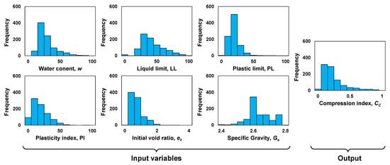
Figure 1.
Histogram of the variables in the dataset.
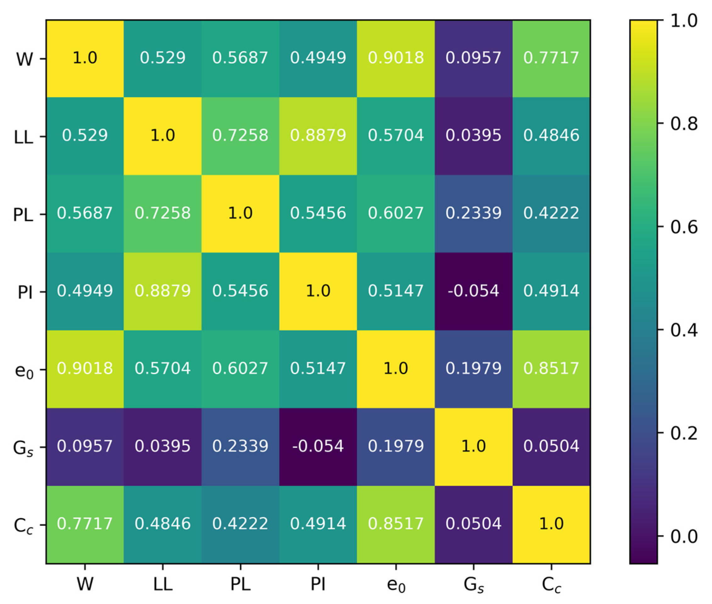
A statistical tool known as Spearman’s correlation coefficient was used to measure the direction and degree of the relationship between two variables. The coefficient value for these variable spans from −1 to 1, with 1 representing a fully positive monotonic connection, −1 representing a fully negative monotonic relationship, and 0 indicating the absence of a monotonic relationship between the variables. Figure 2 shows a Spearman’s correlation coefficient matrix of all the parameters in the dataset in this study. The p-value was used to assess whether the correlation between two variables was statistically significant. Generally, if the p-value is 0.05 or lower, the relationship is considered non-random and statistically significant. Figure 3 demonstrates the Spearman’s correlation coefficient p-value matrix of all the parameters in the dataset in this study. Table 3 lists Spearman’s correlation coefficient and its p-value for the input parameters LL, w, PL, PI, Gs, and e0 and the output parameter, Cc.
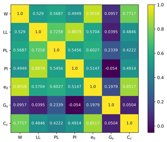
Figure 2.
Matrix of Spearman’s correlation coefficient.
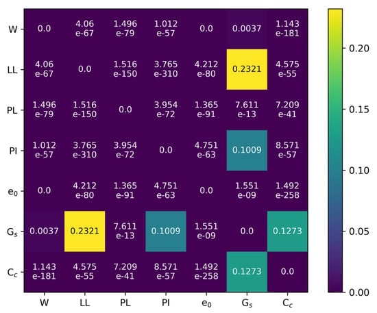
Figure 3.
Spearman’s correlation coefficient p-value matrix.
Table 3.
Spearman’s correlation coefficient and its p-value with compression index.
2.2. Machine Learning Algorithms
The field of machine learning (ML) encompasses the development of algorithms with the capacity to learn and make predictions from data without human intervention. Essentially, machine learning algorithms discover patterns and relationships by analyzing datasets and use this information to make predictions or decisions on new data. Among the most prevalent uses of machine learning is regression. Regression is a machine learning task that aims to predict numerical values. For example, predicting the cost of a house based on its characteristics (e.g., size, location, and age) is a regression problem. The algorithm learns the relationship between features and target values in the given dataset and uses this information to make predictions on new data. Regression is used in a variety of areas, from financial forecasting to risk assessments in the healthcare industry.
The success of machine learning depends on selecting the right datasets, using effective algorithms, and constantly evaluating the performance of the model. This process is becoming increasingly important in more industries due to its capacity to understand and analyze the complexity and diversity of data [48,49].
Machine learning algorithms such as random forest, gradient boosting, and AdaBoost each have their own strengths and weaknesses. The random forest algorithm reduces the risk of overfitting by using multiple decision trees and generally produces more stable results. However, when the model contains too many trees, the training time can be longer, and its performance may slow down on large datasets. The gradient boosting algorithm can provide high accuracy by correcting errors at each step and is particularly effective on complex datasets. However, its downside is that training can be time-consuming, and it may be prone to overfitting. The AdaBoost algorithm focuses on boosting simple models; while it can be effective on low-complexity datasets, it is sensitive to noisy data and may amplify small errors in the dataset. The choice of these models depends on the structure of the dataset and the nature of the problem.
2.2.1. The Random Forest Regressor Algorithm
The random forest regressor algorithm, first created by Breiman [50] and then expanded upon by Geurts et al. [51], is an ensemble learning technique that generates several decision trees during the training process and calculates the average prediction of these trees for regression problems. Each tree is built with randomly selected samples from the training set (e.g., bootstrap sample), and at each node, the best split is selected from a random subset of features, introducing useful randomness into the model [50]. Geurts et al. [51] extended this concept to Extremely Randomized Trees, where the split thresholds for each feature are randomly selected, adding an additional level of randomness. This approach provides a model that is effectively resistant to overfitting, an advantage derived from random feature selection and averaging the predictions from several trees. Although they are capable of modeling complex relationships with high accuracy, random forests can be computationally demanding, especially when composed of many large and deep trees. This method provides improved prediction accuracy and stability in regression tasks due to the combination of decision trees’ simplicity and ensembles’ power.
2.2.2. The Gradient Boosting Regressor Algorithm
Gradient boosting is a popular ML technique for both regression and classification. The model is built incrementally, meaning every new model is constructed with the purpose of rectifying errors caused by the preceding versions. The fundamental principle involves the amalgamation of many weak learners to construct a robust learner, usually decision trees. This algorithm generally starts with a constant, F0(x), aiming to minimize the loss function. Then, at each stage m up to stage ‘m’, a decision tree hm(x) is adapted to the loss function’s negative gradient, the basis of the gradient boosting process. The model is iteratively revised with the learning rate v, which scales the contribution of each tree [52,53]. The equation of the model is demonstrated in Equation (1).
After ‘m’ iterations, the final model, F(x), emerges as the sum of the initial model and all subsequent learners. Stochastic gradient boosting, an extension of this method, adds randomness by subsampling the training data at each stage, thereby increasing the robustness and generalization ability of the model [53]. As highlighted by [48], this approach is part of a broad ensemble learning framework in which each new tree is built on the sum of all previous trees, minimizing the overall prediction error. This structured methodology allows gradient boosting to effectively handle complex nonlinear interactions, making it a versatile tool for regression and classification in various data types.
2.2.3. The AdaBoost Regressor Algorithm
Conceptualized by Freund and Schapire [54] and further developed by Drucker [55], AdaBoost regression represents a significant advance in ensemble learning techniques. Initially, the algorithm assigns equal weights to all training samples, and these weights are dynamically adjusted in subsequent iterations to emphasize the importance of each sample, a method detailed by Freund and Schapire [54]. The basis of the algorithm lies in sequentially integrating weak learners, usually decision trees; the training of each learner is based on the current weight distribution of the samples. This training allows the model to progressively concentrate on more difficult parts of the data, highlighting samples that are difficult to predict. After training each learner, AdaBoost updates the sample weights, increasing them for incorrectly predicted samples and decreasing them for correctly predicted ones; the amount of updating is determined by the accuracy of the learner.
Drucker’s contribution to regression applications of AdaBoost concerns its adaptation with a customized loss function suitable for regression tasks, which led to the AdaBoost R2 algorithm. This adaptation minimizes the specific regression losses, usually by using squared error or absolute error loss functions, thus customizing the algorithm more effectively for continuous outcome prediction. In this context, the overarching objective of AdaBoost is to iteratively enhance the model’s focus on the most difficult-to-predict samples, thus increasing the model’s overall predictive ability across the dataset. The final model, containing the weighted total of all weak learners’ predictions, is robust and accurate, especially in scenarios where the data present complex and nuanced relationships. This adaptive and iterative approach of AdaBoost, especially in its specific form for regression, highlights its effectiveness in handling diverse and complex prediction tasks in various domains.
2.3. Performance Metrics of Regression
The performance metrics of regression are used to measure a model’s predictive ability. The most common error metrics include the mean absolute error (MAE), mean squared error (MSE), root mean squared error (RMSE), and R-squared (R2). In Equation (2), MAE is defined as the mean of the differences between the predicted values and the actual values. The MSE, as shown in Equation (3), is the mean of the squared errors, while the RMSE, as shown in Equation (4), measures the magnitude of the prediction errors by taking the square root of the MSE. Lower MAE, MSE, and RMSE values indicate a better model performance. R-squared, also known as the coefficient of determination, shows how much of the data’s variation the model can explain; its value ranges from 0 to 1, with a higher value indicating a better model. These metrics are critical for assessing the accuracy of the model’s predictions and understanding how closely they align with the actual values, as shown in Equation (5).
2.4. Outline of the Research and Analysis Procedures
We conducted all our research and analysis in this study using the software development environment Visual Studio Code (Version 1.93, Microsoft [56]). The programming language used in this environmental was Python3 (Van Rossum and Drake [57]). We implemented all the machine learning algorithms and calculated the resulting metrics using Scikit-Learn, a Python3 machine learning library (Pedregosa et al. [58]). Figure 4 illustrates the flowchart of the entire research and analysis process.
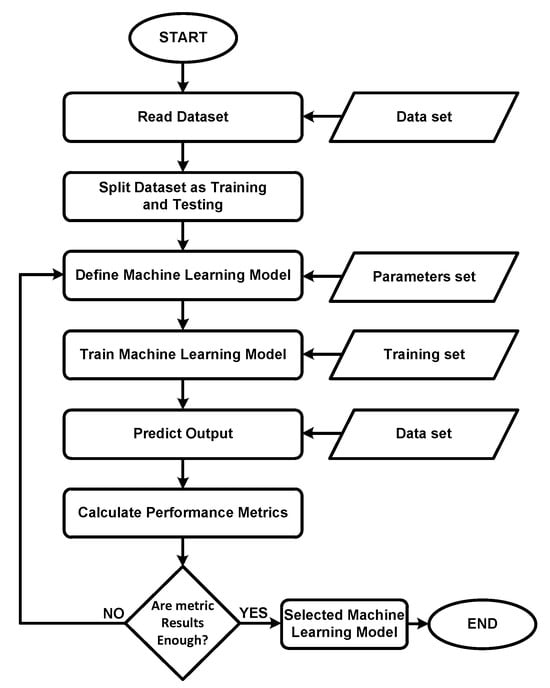
Figure 4.
Flowchart of all research and analysis procedures.
First, the process of loading the dataset into the software development environment, referred to as reading the dataset, was performed. Then, training and testing sets were created from the dataset. A model was defined according to the parameter set, trained with the training set, and used to predict the outputs with the testing set. Subsequently, the performance metrics of the predicted results were calculated. If the metric results were satisfactory, the most appropriate machine learning model was selected.
3. Results
Machine learning algorithms have variables called parameters, similar to mathematical equations. Just as changing the value of a variable in a mathematical equation alters the result, the same applies to machine learning algorithms. Therefore, each algorithm used in the study was trained and evaluated with the parameters LL, w, PL, PI, Gs, and e0 and the compression index (Cc) using the same training and testing sets.
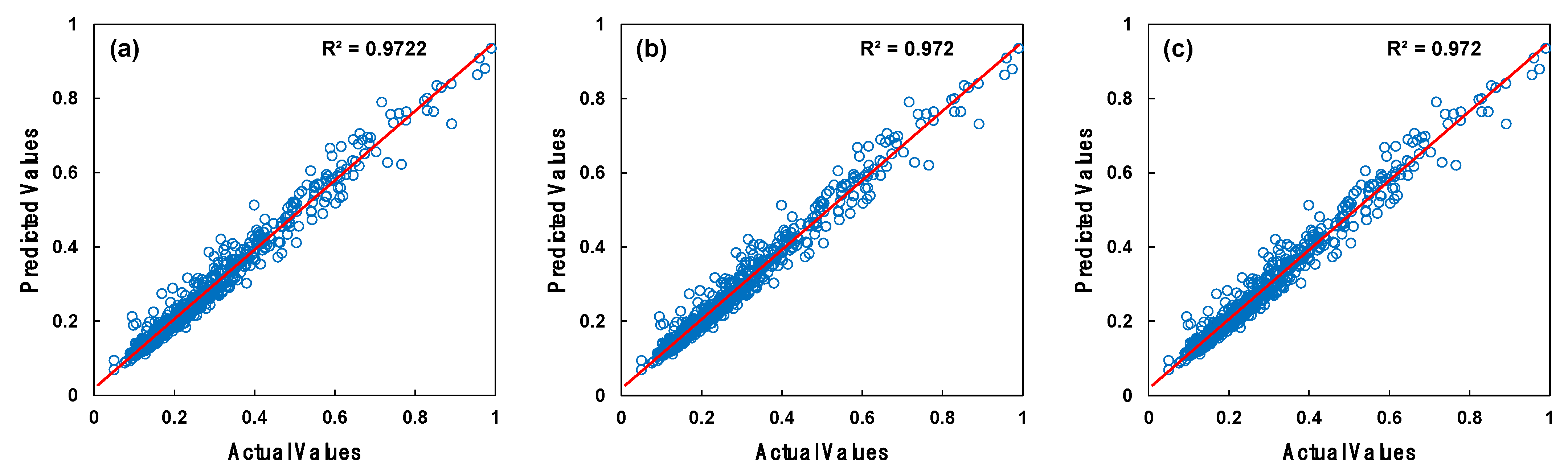
One of purposes of this study was to identify the parameter values that yielded the best outcomes by assigning different values to three parameters of the random forest regressor algorithm: the number of estimators, the number of maximum features, and the maximum depth of the tree. For the parameter of the number of estimators, which indicates the number of trees in the random forest, we used integer values of 10, 50, 100, 200, and 400, respectively. For the parameter of the number of maximum features, which determines the number of features to consider when seeking the best split, we used the options no change (1.0), square root, and logarithmic change. For the maximum depth of the tree parameter, we used integer values of 10, 20, 30, 40, and 50, respectively. Figure 5 and Figure 6 show the training and testing outcomes with blue circle symbols of the best parameter search for the random forest regressor algorithm. The optimal training R2 value of 0.970 and testing R2 value of 0.926 for the random forest regressor were obtained with the parameters number of estimators = 100, number of maximum features = 1.0, and maximum depth = 20.
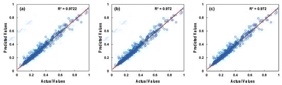
Figure 5.
Training results of the random forest regressor parameter search: (a) the most successful selection, (b) the second most successful selection, and (c) the third most successful selection.
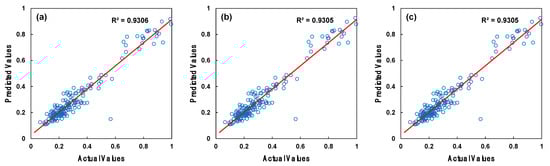
Figure 6.
Testing results of the random forest regressor parameter search: (a) the most successful selection, (b) the second most successful selection, and (c) the third most successful selection.
We aimed to identify the optimal values by experimenting with different values for the loss and learning rate parameters of the gradient boosting regressor algorithm. The learning rate parameter was set to multiples of 10 between and . For the loss function parameter, we employed loss functions including the squared error, absolute error, Huber loss, and quantile. Figure 7 and Figure 8 display the training and testing outcomes with blue circle symbols from the optimal parameter search for the gradient boosting regressor algorithm. The highest training R2 of 0.925 and the highest testing R2 of 0.930 for the gradient boosting regressor were achieved with the parameters set to a learning rate and using a squared error loss function.
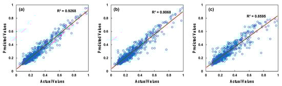
Figure 7.
Training results of the gradient boosting regressor parameter search: (a) the most successful selection, (b) the second most successful selection, and (c) the third most successful selection.
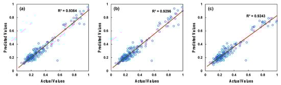
Figure 8.
Testing results of the gradient boosting regressor parameter search: (a) the most successful selection, (b) the second most successful selection, and (c) the third most successful selection.
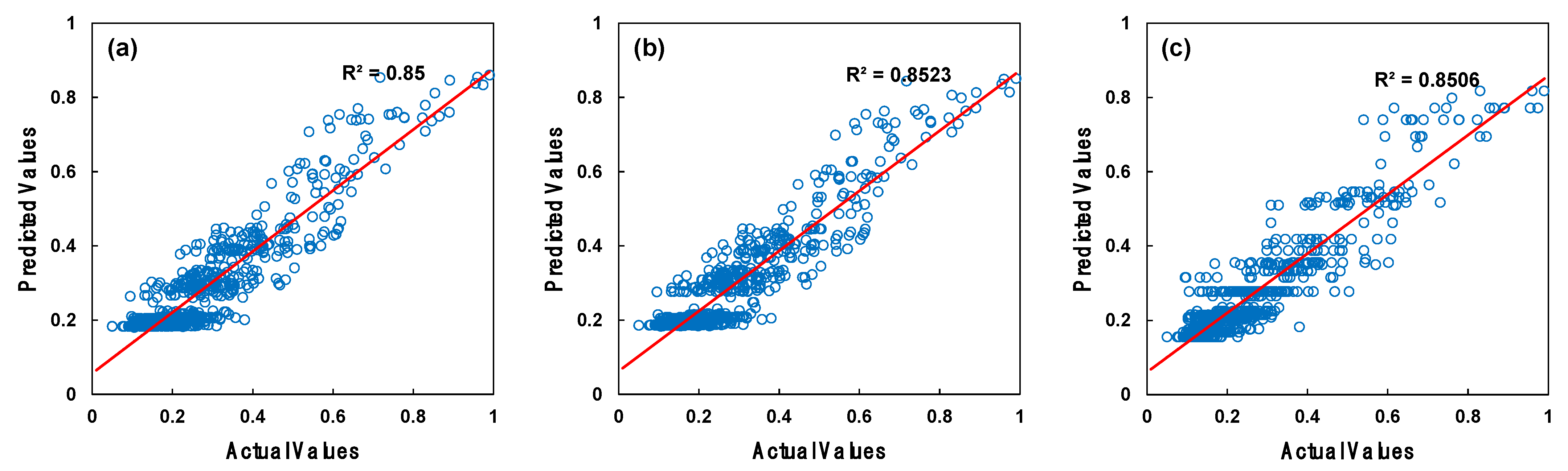
Experiments were conducted with various values for three parameters of the AdaBoost regressor algorithm—the learning rate, loss function, and number of estimators—to achieve the optimal performance. The learning rate parameter was adjusted to 1.0, 0, and multiples of 10 between and . We set the parameter of the number of estimators to integer values of 10, 50, 100, 200, and 400. For the loss function parameter, we applied linear, square, and exponential loss functions.
Figure 9 and Figure 10 present the training and testing results with bule circle symbols obtained during the optimal parameter search for the AdaBoost regressor algorithm. The AdaBoost regressor achieved an optimal training R2 value of 0.847 and testing R2 value of 0.921 with the following parameters: 200 estimators, a learning rate of 1.0, and a square loss function. Table 4 displays the training and testing R2 results for the top three selections, which had the highest values, obtained using different parameter combinations with the algorithms used in this study.
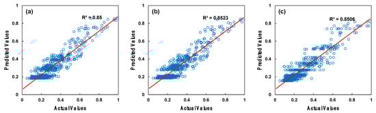
Figure 9.
Training results of the AdaBoost regressor parameter search: (a) the most successful selection, (b) the second most successful selection, and (c) the third most successful selection.
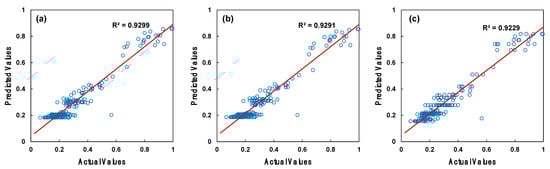
Figure 10.
Testing results of the AdaBoost regressor parameter search: (a) the most successful selection, (b) the second most successful selection, and (c) the third most successful selection.
Table 4.
The R2 results obtained from the training and testing of various parameter combinations.
We tested all combinations of the six inputs in our dataset one by one for the random forest regressor, gradient boosting regressor, and AdaBoost regressor algorithms. The combinations we tried, totaling 63 all in all, were as follows: single-input combinations ([w], [PL], [LL], etc.), two-input combinations ([w, PL], [w, LL], etc.), three-input combinations ([w, PL, LL], etc.), four-input combinations ([w, PL, LL, PI], etc.), five-input combinations ([w, PL, LL, PI, e0], etc.), and six-input combinations ([w, PL, LL, PI, e0, Gs]). Ignoring a few combinations that had very small differences of 0.002, the six-input combination, which included all the inputs in the dataset, showed the most successful results for all three algorithms. Table 5 displays only the highest training and testing R2 results obtained with different input combinations of the algorithms used in this study.
Table 5.
The R2 results obtained from the training and testing of various input combinations.
The random forest regressor with the six-input combination ([w, PL, LL, PI, e0, Gs]) achieved impressive R2 scores of 0.970 for training and 0.926 for testing. The gradient boosting regressor performed slightly better in testing with a four-input combination ([PL, LL, e0, Gs]), with a training R2 score of 0.916 and testing R2 score of 0.932, while the six-input combination yielded a marginally higher training R2 value of 0.925 but a slightly lower testing R2 value of 0.930. The AdaBoost regressor lagged slightly behind when using the six-input combination, with training and testing R2 scores of 0.847 and 0.921, respectively.
4. Discussion
When comparing the results obtained in the current study with those from similar studies in the literature, the three different algorithms used in our study stand out. Table 6 presents a comparison of this study and other works from the literature based on the testing R2 values obtained for predicting results using different algorithms and input parameters. Park and Lee [27] used artificial neural networks (ANNs) and achieved an R2 value of 0.885. Benbouras et al. [36] obtained R2 values of 0.562 with artificial neural networks, 0.360 with genetic programming, and 0.409 with multiple regression analysis. Tsang et al. [37] achieved R2 values of 0.833 with extreme gradient boosting and 0.818 with random forest methods. Chia et al. [38] reported an R2 value of 0.860 with random forest and a higher value of 0.890 with a gradient boosting tree, using a smaller number of parameters. Lastly, Kim et al. [39] reported an R2 value of 0.905 using artificial neural networks.
Table 6.
Comparison of the results of the testing R2 between this study and previous studies.
In this study, an impressive R2 value of 0.926 was achieved with the random forest model, while the gradient boosting and AdaBoost models showed R2 values of 0.930 and 0.921, respectively. Overall, the current study achieves superior results compared to those reported in the literature, particularly when using a comprehensive set of input parameters [w, LL, PL, PI, e0, Gs], highlighting the potential of the methods used in this study to improve the prediction performance.
5. Conclusions
The assessment of fine-grained soils settling under loads, such as buildings, vehicles, and infrastructure, heavily relies on the compression index (Cc). Calculating the Cc parameter is therefore crucial for determining the settlement in soil layers. However, using traditional methods, such as oedometer testing, to measure the value of Cc is time-consuming, requires specialized laboratory equipment, and needs expert staff. Predicting Cc values using additional fine-grained soil characteristics like w, PL, LL, PI, e0, and Gs can save time and costs compared to oedometer testing. In this study, machine learning algorithms, a subfield of artificial intelligence, were employed to estimate the values of Cc using these parameters. A dataset of 915 samples containing these parameters was used to train and test the model. This approach aims to assist geotechnical researchers in calculating the compression index (Cc) more efficiently, thereby saving time and reducing costs.
The compression index is crucial for soil consolidation computations in geotechnical engineering, especially for fine-grained soils. Various machine learning models have been used to predict this coefficient based on different soil properties, providing valuable insights into their relationships with the compression index. This study evaluated the effectiveness of machine learning techniques such as a random forest regressor, gradient boosting regressor, and AdaBoost regressor in predicting the compression index, highlighting the impact of the findings.
The machine learning algorithms in this study were tested with different parameters and various combinations of input parameters to determine the best results. The random forest regressor model demonstrated a significant coefficient of determination (R2) of 0.970 during training and 0.926 during testing when it was trained with the inputs [w, PL, LL, PI, e0, Gs], using parameters such as a maximum depth of 20, a maximum number of features of 1.0, and 100 estimators. The gradient boosting regressor model achieved R2 values of 0.925 for training and 0.930 for testing when trained with the same inputs and parameters, specifically at a learning rate of 0.1 and with a squared error loss function. The AdaBoost regressor model achieved R2 values of 0.847 for training and 0.921 for testing with the inputs [w, PL, LL, PI, e0, Gs] and parameters including 200 estimators, a learning rate of 1.0, and a square loss function. These results indicate that the input parameters—w, PL, LL, PI, e0, and Gs—are effective for successfully predicting the compression index (Cc). When compared with similar studies in the literature, this study achieved higher testing R2 results.
Traditional methods, such as empirical equations, do not typically report performance metrics like R2 because they do not directly focus on the data fit or model optimization. As a result, R2 values can only be calculated and compared for data-driven modeling techniques, such as machine learning algorithms. Machine learning algorithms reduce costs and shorten project durations by making fast and accurate predictions in geotechnical engineering. Compared to the traditional methods, these approaches provide reliable results in complex ground conditions, detect potential risks in advance, and enable safer designs. In this way, structural problems can be prevented in the long term.
This study demonstrated that machine learning models offer valuable insights into understanding the relationships between soil properties and the compression index (Cc). However, it also highlights the risk of overfitting, particularly when there is a significant disparity between the training and testing data. This underscores the importance of exploring other machine learning models or input combinations to improve the compression index predictions. Addressing these model limitations and exploring alternative methodologies can enhance the accuracy and reliability of soil consolidation predictions relevant to geotechnical engineering.
In future work, we plan to explore dimensionality reduction techniques, such as Principal Component Analysis (PCA) or t-SNE, to improve the efficiency of our machine learning models when applying them to high-dimensional geotechnical datasets. The current literature highlights that these methods reduce the computational complexity while preserving the data structure. For example, the book by Lespinats et al. [59] and the work by Van Der Maaten et al. [60] discuss the potential of dimensionality reduction techniques to improve the model performance and enhance our understanding of soil behavior in detail. Incorporating such methods may provide valuable insights to further improve the estimation of the compaction index (Cc).
Author Contributions
Conceptualization, M.K. and M.A.S.; methodology, M.A.S.; software, M.A.S.; validation, M.K., L.L., and M.A.S.; formal analysis, M.K.; investigation, M.K.; resources, L.L.; data curation, M.A.S.; writing—original draft preparation, M.K. and M.A.S.; writing—review and editing, M.K. and L.L.; visualization, M.K. and M.A.S.; supervision, M.K. and L.L; project administration, M.K. and M.A.S.; funding acquisition, L.L. All authors have read and agreed to the published version of the manuscript.
Funding
This research received no external funding.
Institutional Review Board Statement
Not applicable.
Informed Consent Statement
Not applicable.
Data Availability Statement
The data presented in this study are available on request from the corresponding author. The data are not publicly available due to privacy.
Conflicts of Interest
Author Liang Li is employed by the company Terracon Consultants, Inc. The remaining authors declare that the research was conducted in the absence of any commercial or financial relationships that could be construed as a potential conflict of interest.
References
- Sridharan, A.; Sivapullaiah, P.V. Engineering behaviour of soils contaminated with different pollutants. In Environmental Geotechnics, 1st ed.; CRC Press: Boca Raton, FL, USA, 1997; pp. 165–178. [Google Scholar]
- He, Y.; Hu, G.; Wu, D.Y.; Zhu, K.F.; Zhang, K.N. Contaminant migration and the retention behavior of a laterite–bentonite mixture engineered barrier in a landfill. J. Environ. Manag. 2022, 304, 114338. [Google Scholar] [CrossRef] [PubMed]
- Wang, C.; Liu, S.; Shi, X.; Cui, G.; Wang, H.; Jin, X.; Fan, K.; Hu, S. Numerical modeling of contaminant advection impact on hydrodynamic diffusion in a deformable medium. J. Rock Mech. Geotech. Eng. 2022, 14, 994–1004. [Google Scholar] [CrossRef]
- Wolkowski, R.P. Relationship between wheel-traffic-induced soil compaction, nutrient availability, and crop growth: A review. J. Prod. Agric. 1990, 3, 460–469. [Google Scholar] [CrossRef]
- Nawaz, M.F.; Bourrie, G.; Trolard, F. Soil compaction impact and modelling. A review. Agron. Sustain. Dev. 2013, 33, 291–309. [Google Scholar] [CrossRef]
- Shaheb, M.R.; Venkatesh, R.; Shearer, S.A. A review on the effect of soil compaction and its management for sustainable crop production. J. Biosyst. Eng. 2021, 46, 417–439. [Google Scholar] [CrossRef]
- Das, B.H. Principles of Geotechnical Engineering, 7th ed.; Cengage Learning: Stamford, CT, USA, 2009. [Google Scholar]
- Fredlund, D.G.; Rahardjo, H. Soil Mechanics for Unsaturated Soils; John Wiley & Sons: Hoboken, NJ, USA, 1993. [Google Scholar]
- Holtz, R.D.; Kovacs, W.D.; Sheahan, T.C. An Introduction to Geotechnical Engineering, 2nd ed.; Prentice-Hall: Hoboken, NJ, USA, 2011. [Google Scholar]
- Atkinson, J. The Mechanics of Soils and Foundations; CRC Press: Boca Raton, FL, USA, 2017. [Google Scholar]
- Terzaghi, K.; Peck, R.B.; Mesri, G. Soil Mechanics in Engineering Practice; John Wiley & Sons: Hoboken, NJ, USA, 1996. [Google Scholar]
- Sowers, G.B.; Sowers, G.F. Introductory Soil Mechanics and Foundations; Macmillan: New York, NY, USA, 1951. [Google Scholar]
- Nishida, Y. A brief note on compression index of soil. J. Soil Mech. Found. Div. 1956, 82, 1027. [Google Scholar] [CrossRef]
- Yamagutshi, H.T.R. Characteristics of alluvial clay. Rep. Kyushyu Agric. Investig. Cent. Jpn. 1959, 5, 349–358. [Google Scholar]
- Shouka, H. Relationship of compression index and liquid limit of alluvial clay. In Proceedings of the 19th Japan Civil Engineering Conference, Touhoku, Japan, 30–31 May 1964. [Google Scholar]
- Schofield, A.N.; Wroth, P. Critical State Soil Mechanics; McGraw-Hill: New York, NY, USA, 1968. [Google Scholar]
- Ozdikmen, A. Statistical Forecasting of Compression Index. Master’s Thesis, Middle East Technical University, Ankara, Turkey, 1972. [Google Scholar]
- Azzouz, A.S.; Krizek, R.J.; Corotis, R.B. Regression analysis of soil compressibility. Soils Found. 1976, 16, 19–29. [Google Scholar] [CrossRef]
- Koppula, S.D. Statistical estimation of compression index. Geotech. Test. J. 1981, 4, 68–73. [Google Scholar] [CrossRef]
- Nagaraj, T.S.; Srinivasa Murthy, B.R. Prediction of the preconsolidation pressure and recompression index of soils. Geotech. Test. J. 1985, 8, 199–202. [Google Scholar] [CrossRef]
- Pandian, N.S.; Nagaraj, T.S. Critical reappraisal of colloidal activity of clays. J. Geotech. Eng.-ASCE 1990, 116, 285–296. [Google Scholar] [CrossRef]
- Al-Khafaji, A.W.N.; Andersland, O.B. Equations for compression index approximation. J. Geotech. Eng.-ASCE 1992, 118, 148–153. [Google Scholar] [CrossRef]
- Sridharan, A.; Nagaraj, H.B.; Prasad, P.S. Liquid limit of soils from equilibrium water content in one-dimensional normal compression. Proc. Inst. Civ. Eng.-Geotech. Eng. 2000, 143, 165–169. [Google Scholar] [CrossRef]
- Nagaraj, T.S.; Miura, N. Soft Clay Behaviour Analysis and Assessment; CRC Press: Boca Raton, FL, USA, 2001. [Google Scholar]
- Lav, M.A.; Ansal, A.M. Regression analysis of soil compressibility. Turk. J. Eng. Environ. Sci. 2001, 25, 101–109. [Google Scholar]
- Yoon, G.L.; Kim, B.T. Regression analysis of compression index for Kwangyang marine clay. KSCE J. Civ. Eng. 2006, 10, 415–418. [Google Scholar] [CrossRef]
- Park, H.I.; Lee, S.R. Evaluation of the compression index of soils using an artificial neural network. Comput. Geotech. 2011, 38, 472–481. [Google Scholar] [CrossRef]
- Mosavi, A.; Ozturk, P.; Chau, K.W. Flood prediction using machine learning models: Literature review. Water 2018, 10, 1536. [Google Scholar] [CrossRef]
- Torabi, M.; Mosavi, A.; Ozturk, P.; Varkonyi-Koczy, A.; Istvan, V. A hybrid machine learning approach for daily prediction of solar radiation. In Proceedings of the 17th International Conference on Global Research and Education, INTER-ACADEMIA 2018, Kaunas, Lithuania, 24–27 September 2018. [Google Scholar]
- Choubin, B.; Moradi, E.; Golshan, M.; Adamowski, J.; Sajedi-Hosseini, F.; Mosavi, A. An ensemble prediction of flood susceptibility using multivariate discriminant analysis, classification and regression trees, and support vector machines. Sci. Total Environ. 2019, 651, 2087–2096. [Google Scholar] [CrossRef]
- Daryaei, M.; Kashefipour, S.M.; Ahadian, J.; Ghobadian, R. Modeling the compression index of fine soils using artificial neural network and comparison with the other empirical equations. J. Water Soil. 2010, 5, 312–333. [Google Scholar]
- Farkhonde, S.; Bolouri, J. Estimation of compression index of clayey soils using artificial neural network. In Proceedings of the 5th National Congress on Civil Engineering, Mashhad, Iran, 4 May 2010. [Google Scholar]
- Kumar, V.P.; Rani, C.S. Prediction of compression index of soils using artificial neural networks (ANNs). Int. J. Eng. Res. Appl. 2011, 1, 1554–1558. [Google Scholar]
- Alpaydin, E. Introduction to Machine Learning; MIT Press: Cambridge, MA, USA, 2020. [Google Scholar]
- Zhang, W.; Li, H.; Li, Y.; Liu, H.; Chen, Y.; Ding, X. Application of deep learning algorithms in geotechnical engineering: A short critical review. Artif. Intell. Rev. 2021, 54, 5633–5673. [Google Scholar] [CrossRef]
- Benbouras, M.A.; Kettab Mitiche, R.; Zedira, H.; Petrisor, A.I.; Mezouar, N.; Debiche, F. A new approach to predict the compression index using artificial intelligence methods. Mar. Geores. Geotechnol. 2019, 37, 704–720. [Google Scholar] [CrossRef]
- Tsang, L.; He, B.; Ghorbani, A.; Khatami, S.M.H. Tree-based techniques for predicting the compression index of clayey soils. J. Soft Comput. Civ. Eng. 2023, 7, 52–67. [Google Scholar] [CrossRef]
- Chia, Y.H.; Armaghani, D.J.; Lai, S.H. Predicting Soil Compression Index Using Random Forest and Gradient Boosting Tree. In Proceedings of the Chinese Institute of Engineers (CIE), the Hong Kong Institute of Engineers (HKIE), and the Institution of Engineers Malaysia (IEM) Tripartite Seminar, Taipei, Taiwan, 1 November 2023. [Google Scholar]
- Kim, M.; Senturk, M.A.; Tan, R.K.; Ordu, E.; Ko, J. Deep Learning Approach on Prediction of Soil Consolidation Characteristics. Buildings 2024, 14, 450. [Google Scholar] [CrossRef]
- Baghbani, A.; Choudhury, T.; Costa, S.; Reiner, J. Application of artificial intelligence in geotechnical engineering: A state-of-the-art review. Earth-Sci. Rev. 2022, 228, 103991. [Google Scholar] [CrossRef]
- Qader, Z.B.; Karabash, Z.; Cabalar, A.F. Analyzing geotechnical characteristics of soils in Erbil via GIS and ANNs. Sustainability 2023, 15, 4030. [Google Scholar] [CrossRef]
- Jolfaei, S.; Lakirouhani, A. Sensitivity analysis of effective parameters in borehole failure, using neural network. Adv. Civ. Eng. 2022, 2022, 4958004. [Google Scholar] [CrossRef]
- Ongun, Y.A. Determination of Ankara Clay Compression Index. Master’s Thesis, Gazi University, Ankara, Turkey, 2005. [Google Scholar]
- Kilic, E. Statistical Analysis of Consolidation Parameters. Master’s Thesis, Istanbul Technical University, Istanbul, Turkey, 2007. [Google Scholar]
- Satyanarayana, B.; Satyanarayana, R.C.N.V. Development of empirical Equation for compressibility of marine clays. In Proceedings of the Indian Geotechnical Conference, IGC 2010, Mumbai, India, 16–18 December 2010. [Google Scholar]
- Kahraman, E. Statistical Analysis of Consolidation Parameters with Data Set Increased. Master’s Thesis, Istanbul Technical University, Istanbul, Turkey, 2012. [Google Scholar]
- Kalantary, F.; Kordnaeij, A. Prediction of compression index using artificial neural network. Sci. Res. Essays 2012, 7, 2835–2848. [Google Scholar] [CrossRef]
- Hastie, T. The Elements of Statistical Learning: Data Mining, Inference, and Prediction; Springer: New York City, NY, USA, 2009. [Google Scholar]
- Russell, S.J.; Norvig, P. Artificial Intelligence: A Modern Approach; Pearson: London, UK, 2016. [Google Scholar]
- Breiman, L. Random forests. Mach. Learn. 2001, 45, 5–32. [Google Scholar] [CrossRef]
- Geurts, P.; Ernst, D.; Wehenkel, L. Extremely randomized trees. Mach. Learn. 2006, 63, 3–42. [Google Scholar] [CrossRef]
- Friedman, J.H. Greedy function approximation: A gradient boosting machine. Ann. Stat. 2001, 29, 1189–1232. [Google Scholar] [CrossRef]
- Friedman, J.H. Stochastic gradient boosting. Comput. Stat. Data Anal. 2002, 38, 367–378. [Google Scholar] [CrossRef]
- Freund, Y.; Schapire, R.E. A decision-theoretic generalization of on-line learning and an application to boosting. J. Comput. Syst. Sci. 1997, 55, 119–139. [Google Scholar] [CrossRef]
- Drucker, H. Improving regressors using boosting techniques. In Proceedings of the 14th international Conference on Machine Learning, ICML 1997, Nashville, TN, USA, 8–12 July 1997. [Google Scholar]
- Microsoft. Visual Studio Code—Code Editing. Redefined. Available online: https://code.visualstudio.com/ (accessed on 15 April 2024).
- Van Rossum, G.; Drake, F.L. Python 3 Reference Manual; CreateSpace: Scotts Valley, CA, USA, 2009. [Google Scholar]
- Pedregosa, F.; Varoquaux, G.; Gramfort, A.; Michel, V.; Thirion, B.; Grisel, O.; Blondel, M.; Prettenhofer, P.; Weiss, R.; Dubourg, V.; et al. Scikit-learn: Machine learning in Python. J. Mach. Learn. Res. 2011, 12, 2825–2830. Available online: https://www.jmlr.org/papers/v12/pedregosa11a.html (accessed on 4 August 2024).
- Lespinats, S.; Colange, B.; Dutykh, D. Nonlinear Dimensionality Reduction Techniques: A Data Structure Preservation Approach; Springer: New York City, NY, USA, 2022. [Google Scholar]
- Van Der Maaten, L.; Postma, E.O.; Van Den Herik, H.J. Dimensionality reduction: A comparative review. J. Mach. Learn Res. 2009, 10, 13. [Google Scholar]


Disclaimer/Publisher’s Note: The statements, opinions and data contained in all publications are solely those of the individual author(s) and contributor(s) and not of MDPI and/or the editor(s). MDPI and/or the editor(s) disclaim responsibility for any injury to people or property resulting from any ideas, methods, instructions or products referred to in the content. |
© 2024 by the authors. Licensee MDPI, Basel, Switzerland. This article is an open access article distributed under the terms and conditions of the Creative Commons Attribution (CC BY) license (https://creativecommons.org/licenses/by/4.0/).