Abstract
High-voltage circuit breakers (HVCBs) handle the important tasks of controlling and safeguarding electricity networks. In the case of insufficient data samples, improving the accuracy of the traditional HVCB mechanical fault diagnosis method is difficult, so it poses challenges in meeting performance requirements for mechanical fault diagnosis. In this study, a HVCB fault diagnosis method is introduced. It utilizes a combination of grey wolf optimization (GWO) and multi-grained cascade forest (gcForest) algorithms to resolve these issues and improve the accuracy of HVCB mechanical fault diagnosis. To simplify the original vibration signal, the input feature quantity for the fault diagnosis method is obtained by calculating the energy entropy of the wavelet packet decomposition. The GWO algorithm is employed to optimize the parameters of the gcForest model, leading to identification of the optimum parameter configuration. Subsequently, the diagnostic effect in the case of a small sample size was analyzed through a VS1 vacuum circuit breaker example, and the accuracy reached 95.89%. In the case of unbalanced samples, further analysis and comparison with different methods confirm the feasibility and efficiency of the combination of GWO and gcForest algorithms. This study provides an effective solution for the diagnosis of mechanical faults in HVCBs.
1. Introduction
High-voltage circuit breakers (HVCBs) are a vital part of power supplies because they protect and control power systems. The reliability of their operation directly affects the power system itself. Once a HVCB fault occurs, it may cause significant losses to industrial production and the normal life of urban residents [1,2]. When a circuit breaker is in the process of opening and closing, its components will produce strong impacts, which will easily cause various faults such as jamming of the iron core and fatigue of the closing and opening springs. According to a 2012 international report on high-voltage circuit breakers, mechanical failures accounted for the largest proportion of circuit breaker failures [3]. To ensure normal power system operation, strengthening the detection of mechanical faults in HVCBs is essential, and one of the important steps is the detection of vibration signals [4]. Considerable information about the mechanical state is included in the vibration signals resulting from mechanical friction and vibration during the opening and closing of HVCBs, so detecting the mechanical condition of circuit breakers using nonintrusive vibration signals has been extensively researched [5,6]. Mechanical vibration signals are used to diagnose HVCB mechanical failure in this study.
The analysis of the equipment’s state using artificial intelligence technology and massive data is significant for comprehensively understanding equipment operation. Ullah et al. utilized wavelet coherence analysis and deep learning to accurately identify faults in centrifugal pumps [7]. Siddique et al. employed deep learning in combination with enhanced short-time Fourier transform spectrograms and continuous wavelet transform scalograms to precisely detect and classify pipeline leaks [8]. Data-driven methods have exhibited excellent performance in the diagnosis of mechanical faults in HVCBs in recent years. These methods stand out by exploring the correlation of defect samples and defect types [9]. With advances in intelligent technology, some scientific research results have been obtained in the state detection technology of high-voltage switchgear operating mechanisms and transmission. Niu and Zhao [10] applied a neural network and expert system for fault diagnosis in HVCBs. Miao [11] adopted a wavelet packet and support vector machine (SVM) method to accurately diagnose circuit breaker faults, but its optimization algorithm training is complicated and its ability to generalize is weak. Ye et al. [12] used an attention mechanism capsule convolutional neural network in the domain of HVCB fault diagnosis and reached notable achievements. Pan et al. [13] presented a deep belief network and a strategy of transfer learning for the diagnosis of mechanical faults in HVCBs.
However, the currently used deep learning methods are applied based on the premise of a great many samples, and the effect will decrease when sample numbers are small. Because of the prolonged closed state of most circuit breakers during actual operation, the occurrence of mechanical failures is relatively rare. As a result, it becomes challenging to gather a sufficient number of samples through measuring instruments alone. During field operations, the failure probability of HVCBs is remarkably low, resulting in a scarcity of actual failure samples. Furthermore, various types of mechanical failures in HVCBs occur at different probabilities, with some failures being less likely, resulting in a scarcity of samples for certain types and a significant imbalance in the training data. This scarcity or imbalance of training samples can severely limit the capability of deep learning feature extraction. Therefore, fault diagnosis of HVCBs under real conditions poses a challenge as it becomes a small-sample problem. To address the few-shot fault diagnosis problem with insufficient on-site data, the current main solutions are divided into two aspects: the first it to extend the data, which is not only expensive but also mostly relevant to only normal data, making it difficult to obtain effective fault samples. The second is to rely on few-shot learning methods to achieve a solution [14]. Accurate diagnosis of HVCB faults becomes a challenge with a small sample size.
In response to the above challenges, Zhou and Feng [15] proposed a multi-grained cascade forest (gcForest) integration method based on decision trees. The model has the advantages of easy training, low computational overhead, and high parallel computing potential. Zhang et al. conducted a comparative study of various tree-based fault diagnosis models to demonstrate the accuracy of gcForest in creating a diagnosis with small samples [16]. It has been applied to hyperspectral image classification and in bearing fault diagnosis and other fields [17,18], achieving good results. Xu et al. utilized a hybrid learning model of CNN and gcforest to diagnose bearing faults [19]. Su et al. improved the gcForest algorithm by introducing kernel principal component analysis in cascade forests, which outperforms traditional methods when analyzing the experimental vibration data of flip chips [20]. Although the gcForest model performs well in many applications, the results largely depend on the adjustment of model hyperparameters. Optimization of hyperparameters is rarely studied in the regression and classification tasks of machine learning. In a gcForest model, the selection of hyperparameters such as the maximum number of cascaded layers (m), the quantity of decision trees (c) in each random forest, and the quantity of classifiers (n) in each layer of the cascaded structure significantly affects the performance of the model. Therefore, its parameters can be adjusted through the optimization algorithm, and the optimal parameters of the model can be iteratively searched to improve the model’s diagnostic accuracy [21]. Yu [22] proposed a random forest (RF) algorithm based on an improved harmony search to make RF predictions better. Xu et al. [23] have suggested utilizing the particle swarm optimization (PSO) algorithm for optimization of model parameters and have achieved desirable outcomes. Although the PSO algorithm is widely used and straightforward to implement, it is prone to local optima and may lead to deviations in the results.
For this reason, we propose a model that uses the grey wolf optimization (GWO) algorithm to optimize gcForest parameters for fault diagnosis of HVCBs (henceforth referred to as GWO-gcForest) in the case of insufficient data samples. To the best of the author’s knowledge, this is the first time that the GWO-gcForest model has been applied to the field of HVCB mechanical fault diagnosis. In this research, the vibration signal of the HVCB is subjected to feature extraction to determine characteristic parameters. Subsequently, the parameters m, c, and n of the gcForest model are iteratively optimized using the GWO algorithm, leading to the identification of optimal model parameters. Consequently, a GWO-gcForest fault diagnosis model is established. Using this model, an example analysis is conducted to accurately classify the type of fault in the circuit breaker, thereby validating the efficiency of the proposed approach. Furthermore, the diagnostic capability of the model is assessed in scenarios involving different sample sizes and unbalanced samples, further confirming the method’s efficacy. The main contributions of this study are as follows:
- The vibration signals of different types of faults are subjected to wavelet packet decomposition. The third layer of wavelet packet decomposition coefficients are reconstructed, and the energy entropy of each frequency band is calculated and used as a feature vector.
- A new method based on GWO-gcForest is proposed to address the problem of a small number of samples in HVCB mechanical failures. The method uses the GWO algorithm to iteratively optimize the parameters m, c, and n of the gcForest to determine the best model parameters. Subsequently, the GWO-gcForest fault diagnosis model is established.
- The GWO-gcForest fault diagnosis model is utilized for case analysis. The diagnostic capability of the model is evaluated in cases involving different sample sizes and imbalanced samples, validating the effectiveness of the proposed methodology.
The rest of the paper is structured as follows: Section 2 introduces the principle of the GWO-gcForest model, including the gcForest and GWO algorithms. In Section 3, a HVCB fault diagnostic model is developed based on the GWO-gcForest algorithm. Section 4 presents the experimental analysis of HVCB faults and compares it to other methods. Finally, Section 5 provides the conclusions.
2. Preliminaries
A GWO-gcForest fault diagnosis model is proposed to address the problem of an insufficient diagnosis rate for HVCB faults in the case of insufficient samples. The gcForest model does not require large amounts of training data and the training process is convenient and easy to implement. This section describes the gcForest algorithm and the GWO algorithm.
2.1. gcForest
The gcForest algorithm is a new type of classification algorithm based on the RF. The gcForest algorithm classifies samples on the basis of decision trees. It consists of a multi-grained scanning structure (multi-grained scanning) and a cascade forest structure (cascade forest) used to extract the characteristics of the sample set and represent the learning as a model classifier [24,25].
2.1.1. RF Algorithm
The RF algorithm is an ensemble learning algorithm that can be used to solve classification problems based on bagging. The algorithm employs an integrated classification model, which is composed of a group of decision tree classifiers [26]. The parameter denotes the sample that needs to be classified and denotes a random vector that meets the relationship between the kth decision tree’s independent and identical distribution and the vector represented by the parameter.
Sample will be input directly into the RF, and all the decision trees that have been trained will be used in classifying the sample. Each decision tree in the model independently analyses sample by evaluating its characteristic attributes to determine its classification. Once each decision tree provides its individual classification result, the RF model initiates a centralized voting process, where the result of the classification with the highest number of votes is considered as the final result of classifying the sample being classified [27]. The process is shown in Figure 1. The formula is the classification decision result of the RF:
where represents the decision outcome of RF classification, represent the ith decision tree model, represents the goal variable, denotes the measurement function, and denotes the number of trees.
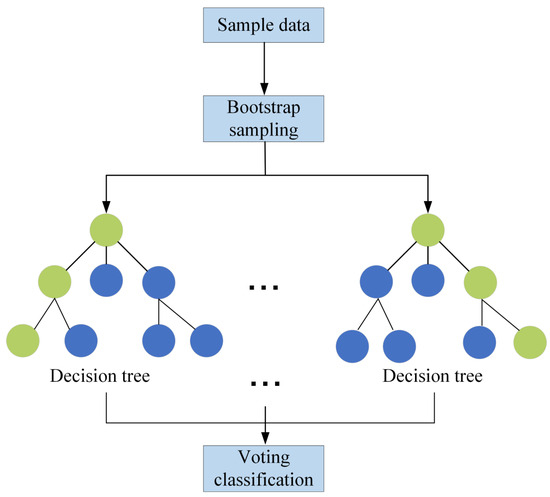
Figure 1.
RF construction process.
2.1.2. Multi-Grained Scanning Structure
Multi-grained scanning is used in the gcForest to mine the characteristics of the sample signal or image [28], and efforts are made to extract the maximum possible characteristic parameters from the sample image.
The multi-grained scanning process closely resembles the convolution process. The sliding window is employed for the extraction of the feature vector. Suppose that input data are N-dimensional and that the sliding window has a dimension of T. By using the sliding window to sample the data, the sampling step can be set to b, and the scanning window count is L, so the number of features is . As a result, a total number of r scanning subsamples is obtained.
Subsequently, the scanning subsamples are separately employed to train different RFs (RF-A and RF-B). As each scanning sample passes through RF-A and RF-B, it generates a probability feature vector dimensioned , where represents the quantity of classes. Finally, the m-dimensional probability feature vectors are concatenated to form the input for the cascaded RF. Details are shown in Figure 2. This scanning structure uses different scanning windows for the original inputs, resulting in multiple features of different dimensions. These features are then trained using RF and complete RF to generate class probability vectors. Finally, these vectors are spliced together.
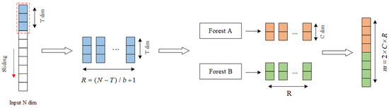
Figure 2.
Multi-grained scanning process.
When actually using the gcForest process, the length of the sliding window can be adjusted, and multiple windows with different lengths can be used to extract features. Data dimensions are expanded through multi-grained scanning as it produces probabilistic feature vectors with rich features.
2.1.3. Cascade Forest Structure
By processing sample features layer by layer, the cascade forest structure improves the algorithm’s feature mining capability, resembling the process of deep learning. This incorporation of deep learning principles enables the cascade forest to effectively extract and refine features for improved performance [29]. It consists of a multi-level RF model, and each level of the RF model contains multiple RFs of different types. This multi-level, multi-dimensional RF processing process for the probability feature vector of input data can effectively improve the characteristic representation ability of input data and contribute to an improvement in accuracy.
Cascade forests use feature information gathered after multi-level scanning as inputs to their first level, and each subsequent level receives the original input and the feature vector connection output from the previous level as the input of this level, so that the feature information is enhanced. There are two RFs per layer of the cascade and two complete RFs per layer. Cross-validation is used to generate the class vectors for each forest, and the output results and the initial input are concatenated and entered at the next level.
In Figure 3, the input represents the m-dimensional probability feature vector produced during the previous section of multi-grained scanning. The category vector generated in the cascade forest stage is called the enhanced feature vector [30]. Next, the enhanced feature vector and the original probability vector are concatenated. The new input feature vector is used as the input feature vector for the next stage. The aforementioned process is repeated until the final layer, where the output average value from the last level’s RF is computed. The category associated with the maximum average output is then selected and designated as the final output. To reduce the risk of overfitting in the gcForest and enhance the model’s generalization capability, it is essential to perform cross-validation on the category vectors generated by each level of the RF within the cascade forest structure.
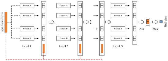
Figure 3.
Cascade forest process.
There is a strong relationship between the quantity of levels in the cascade forest and the performance of the gcForest method. During the process of gcForest construction and training, a certain number of validation datasets can be set, and whenever the number of cascade forest levels increases by one level, the validation datasets are used to test the prediction effect.
2.2. GWO
The GWO algorithm is an intelligent optimization algorithm. It is inspired by the leadership strategy and hunting behavior of grey wolves. During the predation process, grey wolves with a high fitness value can track the position of prey more accurately, guide grey wolves with low fitness to adjust their position, and then prey on the prey through behaviors of encircling, hunting, and attacking [31]. During the optimization process, the PSO algorithm may easily fall into a local optimum, resulting in a large error. Additionally, the GA algorithm has a poor local search ability, leading to low search efficiency. In contrast, the GWO algorithm has a strong convergence performance, few parameters, and is easy to implement.
There is a strict social hierarchy within the grey wolf pack: the α wolf at the top of the pyramid hierarchy is the highest leader, and the other wolves obediently follow the instructions of the α wolf; β and δ wolves mainly obey the α wolf. The layer of wolf conveys the order. The bottom wolf is the ω wolf, obeying the domination of the α, β, and δ wolves, and is mainly responsible for maintaining the harmony and dominant structure of the whole group.
During the process of wolves encircling their prey, the following formula can be used to calculate the distance between an individual grey wolf and its prey:
where represents the actual iteration number, represents the position of the prey, represents the position of the grey wolf individual, and and are vectors representing the coefficients related to synergy. The variables and are random vectors ranging from 0 to 1. Additionally, the coefficient gradually decreases linearly from 2 to 0 during the algorithm’s iterative process.
When wolves are hunting, they surround their prey and recognize its location. In each iteration process, the optimal first three solutions will be kept according to the range from the grey wolf and its prey. According to the positions of the first three solutions, the remaining individuals update their own positions to further search for the optimal solution. An excellent solution is provided by Wang et al. [32]. The specific expressions are
where , , and denote the distances between other individuals and the first three solutions (α, β, δ), respectively, and the wolves can change their positions according to , with
During the optimization process, the α, β, and δ wolves will first approach the prey’s location and then lead the ω wolves to update to the location around the prey. If convergence is achieved, they will attack the prey. The location of the wolves here is the optimal solution.
3. Method of Fault Diagnosis Based on GWO-gcForest for HVCB
In this section, first the process of data processing, followed by the establishment of the HVCB fault diagnosis model, and then the evaluation indexes of the model are proposed.
3.1. Data Processing
The vibration signal is a discrete time series. To further extract its features, the energy entropy of the wavelet packet is used as the quantity of the feature. The processing steps are as follows:
- Decompose the vibration signals of different types of faults into three layers of wavelet packets.
- Reconstruct the wavelet packet decomposition coefficient of the third layer, calculate its energy value, and perform normalization processing. Compute each frequency band’s energy entropy, utilize it as a vector of features, and perform normalization processing on the feature vector. Divide the final feature vectors into training and test sets after normalization.
3.2. Diagnosis Process
The gcForest model is based on tree-based ensemble learning. By integrating the forest composed of trees and connecting them in series, the classifier can perform representation learning, thereby improving the classification effect. Its internal structure can mine fault feature information and identify HVCB faults. However, when employing the gcForest model for fault identification, the determination and control of crucial model parameters rely heavily on human experience. As a result, the diagnostic outcomes are significantly influenced by human manipulation.
With the aim of achieving the utmost diagnostic precision, GWO iteratively searches for optimal model parameters. This iterative process leads to an improvement in the diagnostic accuracy of the model. The process of fault diagnosis on the basis of the GWO-gcForest model comprises three primary phases: data preprocessing, parameter optimization, and fault identification using the optimized model. These steps are illustrated in Figure 4, which shows the overall process.
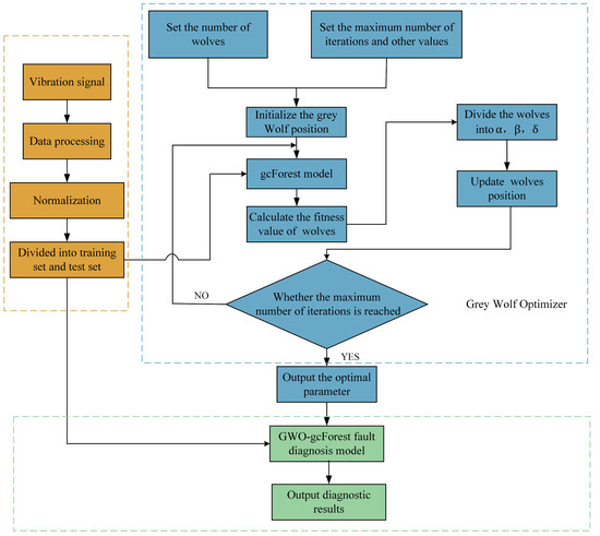
Figure 4.
GWO-gcForest model diagnostic roadmap.
The diagnostic process steps are as follows:
- Obtain vibration signal data. Normalize the features extracted and create a set of training data and a set of test data.
- Initialize the population and determine its size, maximum iteration number, dimensions, and boundary range.
- Construct the gcForest model using the initialized wolves. Train and test the model using the training and testing sets, respectively. Further divide the training set into a verification set. Use the diagnostic accuracy value as the fitness value to assess the model’s performance.
- Calculate the fitness of each wolf, sort each wolf according to the fitness function value, and continually update the wolf pack’s position.
- Halt the GWO process when the fitness value becomes stable or the specified number of iterations is achieved, thereby obtaining the optimal parameters. If neither condition is met, return to the previous step and continue with parameter optimization.
- Build the GWO-gcForest fault diagnosis model using the optimum parameters acquired through the GWO algorithm. Comprehensively analyze the outcomes of the diagnosis, taking into account various evaluation indicators for the assessment of the model’s performance.
3.3. Model Evaluation Index
For analyzing the diagnosis results, the following evaluation indicators were used: precision, recall, F1 value, and accuracy.
Precision is the proportion of accurately predicted labels and the overall number of positive predictions. It can be mathematically represented as follows:
where denotes the overall count of labels and denotes the index of the th label.
Recall is calculated as the proportion of accurately predicted labels to the total count of actual labels, and it can be expressed as follows:
F1 is a comprehensive indicator for precision and recall. There is a negative correlation between precision and recall, and F1 is introduced as a comprehensive index to reconcile the average precision and recall values:
Accuracy is calculated as the proportion of completely accurate predictions to the overall number of samples and can be expressed by the following formula:
where denotes the overall sample size, indicates the index of the th sample, represents the true label, represents the predicted label, and is the indicator function.
4. Discussion and Results of Experiment
This section provides information on the experimental data acquisition process, model parameter selection, and analysis of the experimental results.
4.1. Data Acquisition
For fault diagnosis testing, the VS1 vacuum circuit breaker (Changzhou Senyuan, Changzhou, China) was utilized as the test prototype in this study. The VS1 circuit breaker is a spring-operated mechanism with a rated voltage of 12 kV and a rated current of 1250 A. The vibration signal is collected by a piezoelectric acceleration vibration sensor (YD111T), and the collected charge is converted into a voltage value by a charge amplifier (TS5863). The vibration signal is then transmitted to the upper computer through the acquisition card via the vibration trigger circuit. The experimental equipment is shown in Figure 5.
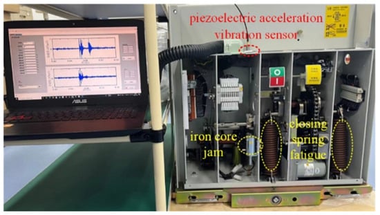
Figure 5.
Experimental equipment setup.
During operation a HVCB may fail, especially in the process of opening and closing. This failure may be caused by electrical or mechanical issues, for example, “refuse to open”, “refuse to close”, “false open”, or “false close”. When such a fault occurs, the circuit breaker has lost the normal function of opening and closing, and these fault phenomena can be easily observed manually. A HVCB can occasionally open and close, but the opening and closing distances of the contacts and the travelling distance after the action cannot reach the normal state. In this study, a total of four working conditions were designed: state 1: normal working condition, state 2: closed spring fatigue failure, state 3: open spring fatigue failure, and state 4: iron core jamming. Shortening the spring tension length by three effective coils (reducing the maximum tension ~8%) can simulate the spring fatigue state. Simulating iron core jamming can be accomplished by adding weights to the electromagnet and to the bolts at the lower end of the movable iron core.
During the test, vibration signals from the operating mechanism of the laboratory were collected under normal conditions and with three mechanical defects. The status signal was derived from the shape of the oscillation signals during opening and closing. Each status sample consisted of 1600 time points, with 40 data samples per defect type. The vibration signals are visually depicted in Figure 6. For dataset partitioning, 60% of the samples were allocated to the training set, 10% to the verification set, and the remaining 30% to the test set. This division ensures a balanced representation of samples across the three sets for training, validation, and evaluation purposes.
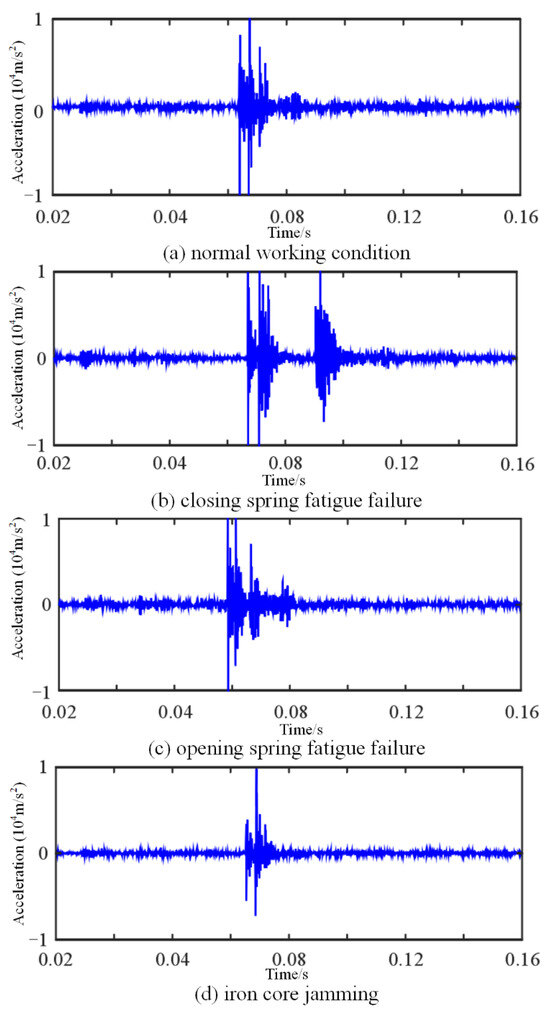
Figure 6.
Vibration signals under (a) normal working condition, (b) closing spring fatigue failure, (c) opening spring fatigue failure, and (d) iron core jamming.
4.2. Setting Experimental Parameters
Experiments were conducted using the Pytorch learning framework on a machine with a GeForce RTX 3070Ti GPU, an Intel i7-13700KF CPU, and 64 GB of memory. To implement the model code, we used Pycharm based on Python 3.9.
In the process of optimizing the model parameters m, c, and n of the GWO-gcForest model, the fitness value of the wolf pack was determined by the training set diagnostic accuracy. The initial setup of the gcForest model consisted of 100 decision trees in each RF. These trees were used for the multi-grain scanning process. The cascade layer had a maximum depth of 20 layers (m), and n was set to 2, resulting in four classifiers in each cascade layer. Additionally, each RF comprised 100 decision trees. For the optimization model, Table 1 provides information regarding the number of populations, maximum number of iterations, and their respective dimensions. The GWO algorithm is iterated 30 times. Three parameters of the gcForest algorithm are optimized to set the GWO dimension to three. The ranges of m, c, and n are related to the parameter sizes within gcForest, and upper and lower bounds are set accordingly.

Table 1.
GWO-gcForest model parameters.
Figure 7 illustrates how the average particle fitness value changes during optimization. Achieving average accuracy optimization of the GWO-gcForest algorithm was improved from 89% to 94% after three steps. Finally, when the maximum depth of the cascade was 7, each classifier was 6, and the number of each forest decision tree was 87.
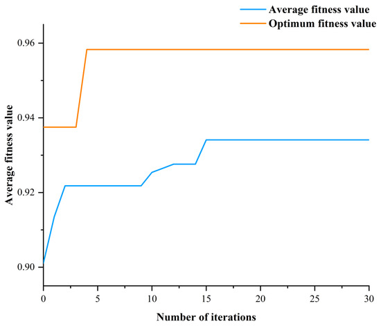
Figure 7.
Particle fitness dependence on the number of iterations.
4.3. Analysis of Experimental Results
In this subsection, a comparison of the performance of GWO-gcForest with other models in the case of different samples as well as in the case of imbalanced samples is provided.
4.3.1. Comparison of Results with Other Models
For the purpose of verifying the superiority of the GWO-gcForest model, we present fault diagnosis accuracies and standard deviations for GWO-gcForest, gcForest, PSO-SVM, SVM, GWO-Randomfroest (GWO-RF), and Randomforest (RF) methods in Figure 8. Based on Figure 8, it is evident that the approach introduced in this research achieves the highest average accuracy of 95.83%. This value surpasses those of other methods, including gcForest, PSO-SVM, SVM, GWO-RF, and RF, by 2.08%, 8.33%, 10.42%, 4.16%, and 6.25%, respectively. This indicates the superior performance and efficiency of the method proposed. There are certain advantages to the proposed methodology regarding accuracy and standard deviation. To analyze the model’s performance further, the various statistical metrics of the method presented in this study are listed in comparison with those of other models in Table 2. Among the evaluation metrics, the GWO-gcForest model proposed in this study achieves the best results. In comparison to gcForest, the remaining three indicators including precision, recall, and F1 increased by 1.89%, 2.08%, and 2.09%, respectively, indicating the effectiveness of model optimization. Furthermore, in comparison to PSO-SVM, it is observed that the proposed model exhibits improvements in precision, recall, and F1 measures by 6.3%, 8.33%, and 8.53%, respectively. These results highlight that the proposed model achieves better overall performance in scenarios involving small sample sizes. Compared with GWO-RF, the three indicators are increased by 2.83%, 4.16%, and 4.32%, respectively, demonstrating the effectiveness of the cascade forest under the optimization algorithm.
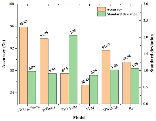
Figure 8.
Accuracies and standard deviations of the models.
Table 2.
Comparison of indicators among different models.
4.3.2. Model Performance with Different Samples
Mechanical failures of HVCBs occur less frequently, and failure samples are scarce in practice. Hence, given the limited availability of samples, there is a need for further research on the fault diagnosis accuracy of HVCBs in scenarios involving small sample sizes. To assess the efficacy of the proposed approach under conditions of limited sample size, the proposed model was used with different sizes of samples and the gcForest, GWO-RF, RF, PSO-SVM, and SVM results were compared with each other. The base unit of the sample size was 40 (100%) per category.
The results are presented in Figure 9. One can see that accuracy gradually decreases as the sample size decreases, with the SVM model dropping the most rapidly as the sample quantity decreases. The GWO-gcForest model accuracy decreases with the decreasing sample size, and the degree of decline is relatively gentle compared with that of other models. The accuracy was ~90% or higher before the sample size dropped to 75%. When the sample size was further reduced to 25%, it is observed that only the method introduced in this study outperforms other models in terms of the accuracy of fault diagnosis. This finding suggests that the proposed model possesses certain advantages even when the number of samples for each fault type is limited. Based on the downward trend of the accuracy rate, the GWO-gcForest model has a better diagnostic effect when the sample size is small.
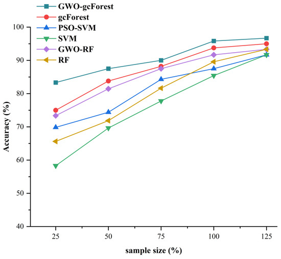
Figure 9.
Accuracy of each algorithm under different sample sizes.
4.3.3. Model Performance on Imbalanced Datasets
HVCBs have different probabilities of occurrence for different types of mechanical failures during operation, but some of them have a very low probability of occurrence.
To evaluate the ability of our proposed method in solving the unbalanced sample problem, taking into consideration the impact of varying sample sizes across different classes on the performance of the model in fault diagnosis, we constructed the unbalanced sample dataset presented in Table 3.
Table 3.
Unbalanced sample datasets used in this study.
By setting the number of samples in states 3 and 4, the imbalance that may exist in practice is simulated. Under the condition of an imbalanced dataset, the performance of various methods was simulated and assessed on the test set. To conduct a detailed analysis of the fault diagnosis capability of the GWO-gcForest model in the presence of imbalanced sample conditions, a comparison was made with other models such as gcForest, GWO-RF, and additional relevant models.
The experimental results are visually presented in Figure 10. As the sample imbalance increases, the accuracy of all the models decreases. However, in comparison to other models, our proposed method demonstrates a higher level of accuracy when handling unbalanced samples. When the imbalance ratio is 40:40:20:10, diagnostic accuracy of the proposed method is 90.91%, while the classification accuracies of other models are all <90%. In the case of dataset 4, the accuracy of the proposed model is still close to 90%. Figure 10 clearly illustrates that, across various unbalanced-sample scenarios, the GWO-gcForest model consistently outperforms other fault diagnosis methods. To provide a clearer analysis of the recognition accuracy under different sample datasets, radar charts depicting the confusion matrix of the four methods were constructed. These radar charts offer a visual representation of the accuracy in classification of each method across different types of data, enabling a more detailed and comprehensive comparison. As depicted in Figure 11, each axis corresponds to a specific sample dataset, and the length of each axis reflects the recognition accuracy of the respective methods for that particular dataset. The analysis reveals that the proposed methodology exhibits outstanding results across different types of datasets.
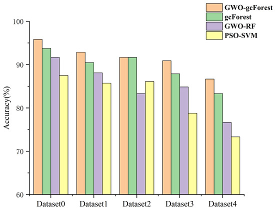
Figure 10.
Results of different models with unbalanced samples.
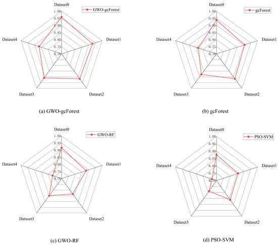
Figure 11.
Confusion radar maps of four methods: (a) GWO-gcForest, (b) gcForest, (c) GWO-RF, and (d) PSO-SVM.
5. Conclusions
This paper presents a case study on the mechanical fault diagnosis of HVCBs. The proposed model accurately diagnoses faults without requiring a large amount of data. The GWO-gcForest model outperforms traditional algorithms such as gcForest, GWO-RF, RF, PSO-SVM, and SVM in the case of small and imbalanced samples. The effectiveness of the fault diagnosis algorithms is demonstrated through cases. This provides a valuable method for the field of fault diagnosis.
A novel model for diagnosing faults in HVCBs on the basis of GWO-gcForest is introduced. The GWO algorithm is used for optimization of the critical parameters of the gcForest model, effectively mitigating random fluctuations in the model’s output and enhancing its generalization ability. By leveraging the power of the GWO algorithm, the performance and reliability of the gcForest model are significantly improved.
Experimental results provide evidence that the proposed approach surpasses gcForest, GWO-RF, and other models mentioned in this study with regard to accuracy. Even when the data sample size is small, the proposed model maintains a high level of accuracy. In addition, it also has good performance under unbalanced sample data, which proves the efficacy and superiority of the method.
The model provides a feasible solution for fault identification of HVCBs, offering promising application prospects. However, this study was conducted in the laboratory under ideal experimental conditions. Improving the practical application of the project for actual operation in the field is a problem that must be solved in our future work.
Author Contributions
Conceptualization, M.Q.; methodology, Z.X. and Y.W.; software, G.S.; validation, J.W. and Y.G.; formal analysis, Z.Z.; investigation, Z.X.; writing—original draft preparation, Z.X. and J.Y.; writing—review and editing, J.Y.; project administration, J.W. and Y.G.; funding acquisition, J.Y. and Y.G. All authors have read and agreed to the published version of the manuscript.
Funding
This research was funded by the National Key Research and Development Program of China grant number [No. 2022YFB2403700].
Institutional Review Board Statement
Not applicable.
Informed Consent Statement
Not applicable.
Data Availability Statement
The data presented in this study are available on request from the corresponding author. The data are not publicly available due to privacy and ethical.
Conflicts of Interest
The authors declare no conflicts of interest.
References
- Chen, L.; Wan, S.T. Intelligent fault diagnosis of high-voltage circuit breakers using triangular global alignment kernel extreme learning machine. ISA Trans. 2021, 109, 368–379. [Google Scholar] [CrossRef] [PubMed]
- Razi-Kazemi, A.A.; Niayesh, K.; Nilchi, R. A Probabilistic Model-Aided Failure Prediction Approach for Spring-Type Operating Mechanism of High-Voltage Circuit Breakers. IEEE Trans. Power Deliv. 2019, 34, 1280–1290. [Google Scholar] [CrossRef]
- Carvalho, A.; Cormenzana, M.L.; Furuta, H.; Grieshaber, W.; Hyrczak, A.; Kopejtkova, D.; Krone, J.G.; Kudoke, M.; Makareinis, D.; Martins, J.F.; et al. Final Report of the 2004–2007 International Enquiry on Reliability of High Voltage Equipment, Part 2—Reliability of High Voltage Equipment; CIGRÉ Technical Brochure No. 512; International Council on Large Electric Systems (CIGRÉ): Paris, France, 2012. [Google Scholar]
- Guan, Y.; Yang, Y.; Zhong, J.; Cheng, T. Review on Mechanical Fault Diagnosis Methods for High-voltage Circuit Breakers. High Volt. Appar. 2018, 54, 10–19. [Google Scholar]
- Attoui, I.; Oudjani, B.; Boutasseta, N.; Fergani, N.; Bouakkaz, M.S.; Bouraiou, A. Novel predictive features using a wrapper model for rolling bearing fault diagnosis based on vibration signal analysis. Int. J. Adv. Manuf. Technol. 2020, 106, 3409–3435. [Google Scholar] [CrossRef]
- Ma, H.Z.; Liu, B.W.; Xu, H.H.; Chen, B.B.; Ju, P.; Zhang, L.; Qu, B. GIS mechanical state identification and defect diagnosis technology based on self-excited vibration of assembled circuit breaker. IET Sci. Meas. Technol. 2020, 14, 56–63. [Google Scholar] [CrossRef]
- Ullah, N.; Ahmad, Z.; Siddique, M.F.; Im, K.; Shon, D.K.; Yoon, T.H.; Yoo, D.S.; Kim, J.M. An Intelligent Framework for Fault Diagnosis of Centrifugal Pump Leveraging Wavelet Coherence Analysis and Deep Learning. Sensors 2023, 23, 8850. [Google Scholar] [CrossRef] [PubMed]
- Siddique, M.F.; Ahmad, Z.; Ullah, N.; Kim, J. A Hybrid Deep Learning Approach: Integrating Short-Time Fourier Transform and Continuous Wavelet Transform for Improved Pipeline Leak Detection. Sensors 2023, 23, 8079. [Google Scholar] [CrossRef]
- Gao, W.; Qiao, S.P.; Wai, R.J.; Guo, M.F. A Newly Designed Diagnostic Method for Mechanical Faults of High-Voltage Circuit Breakers via SSAE and IELM. IEEE Trans. Instrum. Meas. 2021, 70, 3500613. [Google Scholar] [CrossRef]
- Niu, X.; Zhao, X.X. The Study of Fault Diagnosis the High-Voltage Circuit Breaker Based on Neural Network and Expert System. In Proceedings of the International Workshop on Information and Electronics Engineering (IWIEE)/International Conference on Information, Computing and Telecommunications (ICICT), Harbin, China, 10–11 March 2012; pp. 3286–3291. [Google Scholar]
- Miao, D. Research on Fault Diagnosis of High-Voltage Circuit Breaker Based on Support Vector Machine. Int. J. Pattern Recognit. Artif. Intell. 2019, 33, 1959019. [Google Scholar] [CrossRef]
- Ye, X.; Yan, J.; Wang, Y.; Lu, L.; He, R. A Novel Capsule Convolutional Neural Network with Attention Mechanism for High-Voltage Circuit Breaker Fault Diagnosis. Electr. Power Syst. Res. 2022, 209, 108003. [Google Scholar] [CrossRef]
- Pan, Y.; Mei, F.; Miao, H.Y.; Zheng, J.Y.; Zhu, K.D.; Sha, H.Y. An Approach for HVCB Mechanical Fault Diagnosis Based on a Deep Belief Network and a Transfer Learning Strategy. J. Electr. Eng. Technol. 2019, 14, 407–419. [Google Scholar] [CrossRef]
- Jing, Q.; Yan, J.; Wang, Y.; Ye, X.; Wang, J.; Geng, Y. A novel method for small and unbalanced sample pattern recognition of gas insulated switchgear partial discharge using an auxiliary classifier generative adversarial network. High Volt. 2022, 8, 368–379. [Google Scholar] [CrossRef]
- Zhou, Z.H.; Feng, J. Deep Forest: Towards an Alternative to Deep Neural Networks. In Proceedings of the 26th International Joint Conference on Artificial Intelligence (IJCAI), Melbourne, Australia, 19–25 August 2017; pp. 3553–3559. [Google Scholar]
- Zhang, H.; Zhong, C.; Zhang, Z.; Jiang, Y. A comparative study of rolling bearing fault diagnosis based on tree models. In Proceedings of the 2nd International Conference on Digital Society and Intelligent Systems (DSInS 2022), Chendgu, China, 2–4 December 2022; Volume 12599. [Google Scholar] [CrossRef]
- Qin, X.W.; Xu, D.X.; Dong, X.G.; Cui, X.T.; Zhang, S.Q. The Fault Diagnosis of Rolling Bearing Based on Improved Deep Forest. Shock Vib. 2021, 2021, 9933137. [Google Scholar] [CrossRef]
- Zheng, L.; Bao, Q.; Weng, S.Z.; Tao, J.P.; Zhang, D.Y.; Huang, L.S.; Zhao, J.L. Determination of adulteration in wheat flour using multi-grained cascade forest-related models coupled with the fusion information of hyperspectral imaging. Spectrochim. Acta Part A Mol. Biomol. Spectrosc. 2022, 270, 120813. [Google Scholar] [CrossRef] [PubMed]
- Xu, Y.; Li, Z.X.; Wang, S.Q.; Li, W.H.; Sarkodie-Gyan, T.; Feng, S.Z. A hybrid deep-learning model for fault diagnosis of rolling bearings. Measurement 2021, 169, 108502. [Google Scholar] [CrossRef]
- Su, L.; Hu, X.; Gu, J.F.; Ji, Y.; Wang, G.; Ming, X.F.; Li, K.; Pecht, M. Intelligent defect inspection of flip chip based on vibration signals and improved gcForest. Measurement 2023, 214, 112782. [Google Scholar] [CrossRef]
- Huang, J.; Hu, X.G.; Yang, F. Support vector machine with genetic algorithm for machinery fault diagnosis of high voltage circuit breaker. Measurement 2011, 44, 1018–1027. [Google Scholar] [CrossRef]
- Yu, M.X. Short-term wind speed forecasting based on random forest model combining ensemble empirical mode decomposition and improved harmony search algorithm. Int. J. Green Energy 2020, 17, 332–348. [Google Scholar] [CrossRef]
- Xu, C.L.; Li, L.S.; Li, J.W.; Wen, C.A.B. Surface Defects Detection and Identification of Lithium Battery Pole Piece Based on Multi-Feature Fusion and PSO-SVM. IEEE Access 2021, 9, 85232–85239. [Google Scholar] [CrossRef]
- Liu, X.L.; Tian, Y.; Lei, X.H.; Liu, M.; Wen, X.; Huang, H.C.; Wang, H. Deep forest based intelligent fault diagnosis of hydraulic turbine. J. Mech. Sci. Technol. 2019, 33, 2049–2058. [Google Scholar] [CrossRef]
- Liu, K.Z.; Wu, S.Z.; Luo, Z.; Gongze, Z.W.Y.; Ma, X.L.; Cao, Z.G.; Li, H.J. An Intelligent Fault Diagnosis Method for Transformer Based on IPSO-gcForest. Math. Probl. Eng. 2021, 2021, 6610338. [Google Scholar] [CrossRef]
- Yao, H.F.; He, H.; Wang, S.L.; Xie, Z.P. EEG-based Emotion Recognition Using Multi-scale Window Deep Forest. In Proceedings of the 2019 IEEE Symposium Series on Computational Intelligence (SSCI), Xiamen, China, 6–9 December 2019; pp. 381–386. [Google Scholar]
- Ma, S.L.; Chen, M.X.; Wu, J.W.; Wang, Y.H.; Jia, B.W.; Jiang, Y. Intelligent Fault Diagnosis of HVCB with Feature Space Optimization-Based Random Forest. Sensors 2018, 18, 1221. [Google Scholar] [CrossRef]
- Liu, Q.; Gao, H.L.; You, Z.C.; Song, H.L.; Zhang, L. Gcforest-Based Fault Diagnosis Method For Rolling Bearing. In Proceedings of the Prognostics and System Health Management Conference (PHM-Chongqing), Chongqing, China, 26–28 October 2018; pp. 572–577. [Google Scholar]
- Zhang, Z.H.; Guo, F.; Xu, Z.; Yang, X.Y.; Wu, K.Z. On retrieving the chromium and zinc concentrations in the arable soil by the hyperspectral reflectance based on the deep forest. Ecol. Indic. 2022, 144, 109440. [Google Scholar] [CrossRef]
- Chen, H.; Li, C.S.; Yang, W.X.; Liu, J.; An, X.L.; Zhao, Y.J. Deep balanced cascade forest: An novel fault diagnosis method for data imbalance. ISA Trans. 2022, 126, 428–439. [Google Scholar] [CrossRef]
- Mirjalili, S.; Mirjalili, S.M.; Lewis, A. Grey Wolf Optimizer. Adv. Eng. Softw. 2014, 69, 46–61. [Google Scholar] [CrossRef]
- Wang, T.; Zhang, L.; Wu, Y. Research on transformer fault diagnosis based on GWO-RF algorithm. J. Phys. Conf. Ser. 2021, 1952, 032054. [Google Scholar] [CrossRef]
Disclaimer/Publisher’s Note: The statements, opinions and data contained in all publications are solely those of the individual author(s) and contributor(s) and not of MDPI and/or the editor(s). MDPI and/or the editor(s) disclaim responsibility for any injury to people or property resulting from any ideas, methods, instructions or products referred to in the content. |
© 2024 by the authors. Licensee MDPI, Basel, Switzerland. This article is an open access article distributed under the terms and conditions of the Creative Commons Attribution (CC BY) license (https://creativecommons.org/licenses/by/4.0/).