Using Bayesian Regularized Artificial Neural Networks to Predict the Tensile Strength of Additively Manufactured Polylactic Acid Parts

Abstract

Additive manufacturing has transformed the production process by enabling the construction of components in a layer-by-layer approach. This study integrates Artificial Neural Networks to explore the nuanced relationship between process parameters and mechanical performance in Fused Filament Fabrication. Using a fractional Taguchi design, seven key process parameters are systematically varied to provide a robust dataset for model training. The resulting model confirms its accuracy in predicting tensile strength. In particular, the mean squared error is 0.002, and the mean absolute error is 0.024. These results significantly advance the understanding of 3D manufactured parts, shedding light on the intricate dynamics between process nuances and mechanical outcomes. Furthermore, they underscore the transformative role of machine learning in precision-driven quality prediction and optimization in additive manufacturing.

1. Introduction

Additive manufacturing (AM) is revolutionizing production technologies by enabling the creation of components layer by layer without the limitations of traditional manufacturing methods. This technology also allows for the use of a variety of materials, making it highly attractive to industries such as the automotive, aircraft, and medical industries [1,2]. Material extrusion (ME) is a type of 3D printing process that involves selectively depositing material through a heated nozzle [3] and is one of seven categories of additive printing processes defined by the ASTM/ISO 52900 standard [3]. Extrusion-based technology can process a wide range of materials [4], making it suitable also for constructing complex parts [5,6]. Fused Deposition Modeling (FDM), also known as Fused Filament Fabrication (FFF), is a 3D printing process that uses a thermoplastic filament to create components layer by layer. The path of the nozzle is defined by the file codes generated during the design stage. The most used thermoplastic material for FDM is polylactic acid (PLA), made from plant-based sources.

To ensure that FFF-made components meet their functional requirements, critical process factors must be examined to determine their impact on mechanical qualities. Several studies have looked at the influence of the key process parameters. A Taguchi orthogonal array was used to define the level of each factor, and the experimental data were analyzed using analysis of variance (ANOVA) to quantify the main effects of the parameters on the responses [6,7,8]. In a study using Taguchi’s L9, the effects of the printing speed, layer height, and extrusion temperature were analyzed, and the results showed that higher extrusion temperatures improved interlayer adhesion in the printed object. On the other hand, the use of printing speeds that are too high leads to a progressive reduction in the tensile strength because the deposition of the layers is not uniform. The optimal process parameters for this work are a layer height of 0.15 mm, a printing speed of 48 mm/s, and an extrusion temperature of 220 °C [9]. By using lower melting temperatures, at which printing speeds do not affect the geometry of the part, the necessary integrity of the structure is maintained. For the maximum tensile strength, higher extruding temperatures provide better material bonding. Lower printing speeds combined with the printing temperature leads to higher strain and stiffness [10]. Moreover, higher cooling speeds were found to improve the geometric accuracy but decrease the mechanical strength [11]. A detailed analysis of the specimen’s internal structure was conducted to study the effects of infill type, percentage of part fill, number of perimeters, and shell thickness. The performance is influenced by the chosen infill pattern and the number of contours, with optimal values being a layer height of 0.1 mm, six perimeters, and a gyroid infill geometry [12]. In contrast, ranked first in influence is the infill percentage, followed by the contour thickness and then the layer height. In Enemuoh et al.’s study, the most influential parameter for optimum printing was found to be the infill percentage, followed by the contour thickness and layer height. Specifically, an infill density of 100%, a shell thickness of 1.2 mm, a layer thickness of 0.2 mm, a cubic infill pattern, and a print speed of 40 mm/s were identified as optimal printing parameters [13]. The results on layer thickness are mixed. Caminero et al. observed that on-edge and flat orientations result in the highest mechanical properties with intra-layer failure. The study found that the tensile strength was highest at a lower layer thickness, which also had a higher ductility. However, the ductility decreased as the layer thickness increased [14]. Another study showed that increasing the layer height from 0.1 to 0.2 mm resulted in improving the tensile strength. Furthermore, the triangle pattern provides the optimal mechanical strength while minimizing material consumption [15,16].

Machine learning (ML) is a subfield of artificial intelligence (AI) that uses algorithms to analyze data, recognize patterns, and make decisions without explicit instructions. It is based on objective analysis and logical structure. Within the field of ML, artificial neural networks (ANNs) are modeled to simulate the working flow of the human brain and consist of interconnected nodes that mimic neurons. ANNs excel at learning intricate patterns and correlations in data, making them ideal for applications such as image identification, natural language processing, and predictive analytics. The development of deep neural networks has further improved the capability in processing various and complex datasets [17]. ANNs have played a crucial role in image recognition tasks, including object detection, facial recognition, and image classification. This has resulted in significant progress in areas such as self-driving cars, medical imaging, and security systems [18]. Deep learning (DL) differs from traditional ANNs in its ability to automatically learn complex data representations through the use of deep neural networks with many hidden layers. Compared with traditional ML, DL can learn complicated representations of datasets automatically, without the need to manually extract relevant features. It enables more efficient and accurate learning from raw data, automatically uncovering complex patterns and relationships that may not be apparent upon initial analysis. Additionally, it can handle large amounts of data and adapt dynamically to changes, making it particularly suitable for applications with high data complexity and dimensionality [19]. On the other hand, Deep Belief Networks (DBNs) are hierarchically structured ANNs that learn complex representations of input data using probabilistic methods. They have been used successfully in areas such as computer vision, natural language recognition, bioinformatics, and financial data analysis. Recent developments include hybrid architectures that combine DBNs with other deep learning techniques, such as Convolutional Neural Networks (CNNs) for image processing and Recurrent Neural Networks (RNNs) for sequential data processing. This combination improves model performance and increases flexibility when learning data representations. DBNs are increasingly being used on cloud platforms, allowing for more efficient data management and faster neural network training [19]. One of its applications is in smart cities to improve security and efficiency. It enables anomaly detection, data encryption, intrusion detection, behavior analysis, and secure communication with significantly improved overall security by providing effective tools for data protection and cyber threat prevention [20]. Moreover, to enhance the planning and administration of urban tunnel building projects, DBNs are utilized to predict the performance of cantilever roadheaders in challenging terrain. This enables the precise and timely control of factors that affect roadheader performance. The use of DBNs allows one to address issues related to the complexity of geological data and the nonlinear correlations between excavation factors, resulting in more accurate projections that are adaptive to changing ground conditions [21]. High-resolution image processing is crucial in various industries, including medical analysis, satellite image processing, and computer graphics. Rehman et al. [22] proposed a cascade approach, where a CNN extracts DNN-based features from input image patches. These features are then fed into the DBN model for high-resolution image quality prediction. This study aims to improve the objective assessment of super-resolution image quality by providing an advanced, accurate approach without reference images. Bayesian neural networks (BNNs) are a type of neural network that treat model weights as random variables with probability distributions, rather than fixed parameters. This approach captures the uncertainty associated with the model weights and input data, resulting in more informative and robust predictions. Bayesian approaches enable the estimation of the posterior distribution of model parameters from observed data. This estimation can be used for model selection, prediction, and uncertainty quantification. Additionally, Bayesian approaches can improve the generalization performance of ANNs by reducing overfitting and providing a principled method for selecting the appropriate model complexity. Bayesian methods have the advantage of incorporating prior knowledge into the model, which is useful when training data are limited. They are also robust to outliers and less sensitive to overfitting than non-Bayesian methods due to constraints on model complexity [23,24]. The transition from the traditional Bayesian approach to Bayesian regularization (BR) is a significant advancement in the field of neural networks and machine learning. This approach improves network performance, making it more robust and better able to generalize to new data, without the full complexity of traditional Bayesian methods [25,26]. Bayesian analysis is a suitable approach for addressing uncertainties in civil engineering problems such as materials, excitation, modeling, and emission for damage prediction [24]. Moreover, the approach has been utilized to address various challenges in the medical field, including predicting disease progression, identifying diagnostic biomarkers, and customizing treatments to individual patient characteristics [27].

Nowadays, digital technologies and solutions for calibration, prediction, learning, and self-optimization have been implemented in manufacturing to eliminate inefficiencies [28]. The combination of AM and ML techniques offers the ability to identify relationships in large manufacturing datasets, providing the possibility of obtaining components with improved performance [29]. Charalampous et al. [30] investigated tensile strength optimization by adopting an ML regression algorithm. The layer thickness, printing speed, and printing temperature were the process parameters considered. The results showed that a medium printing speed, temperature, and low layer thickness improved the tensile strength. The layer height, infill percentage, printing temperature, and printing speed were used as input to train an ML model for simultaneously predicting the minimum weight, minimum printing time, and maximum tensile strength. Although no unique optimal solution exists, the Pareto front provides an appropriate combination of input parameters to obtain the best trade-off between the outputs to meet the user’s requirements [31]. The same printing processes were investigated by Jatti et al. using an ML nonlinear regression algorithm only for tensile strength prediction. The results were able to predict the tensile strength with a percentage error of less than 2.977 [32]. Models for predicting the ultimate tensile strength were developed using an ANN. The regression curve had a correlation coefficient of 0.999782. The input combinations between the print speed, infill density, build orientation, temperature, and layer thickness were evaluated based on the Taguchi orthogonal array. Having considered for each input three control levels, 33 experiments were performed for the training and evaluation of a neural network. The error percentage value for the neural network is 1.10. The validation parameter indicates an error of 1.57 when comparing the actual and predicted outcomes using the ML method [33]. In the majority of the current study’s results, the best combination of process parameters was discovered through independent experimental trials, with the experimental outcome that produced a better solution being classified as the optimum solution [34]. However, the optimal process parameter combination may differ from the experimental combinations, and it must fall within the permitted range of process parameters [35]. Additionally, FFF involves a large number of process parameters that must be carefully controlled to ensure the proper formation of components. Therefore, it is essential to control the parameters that have an impact on mechanical performance [36].

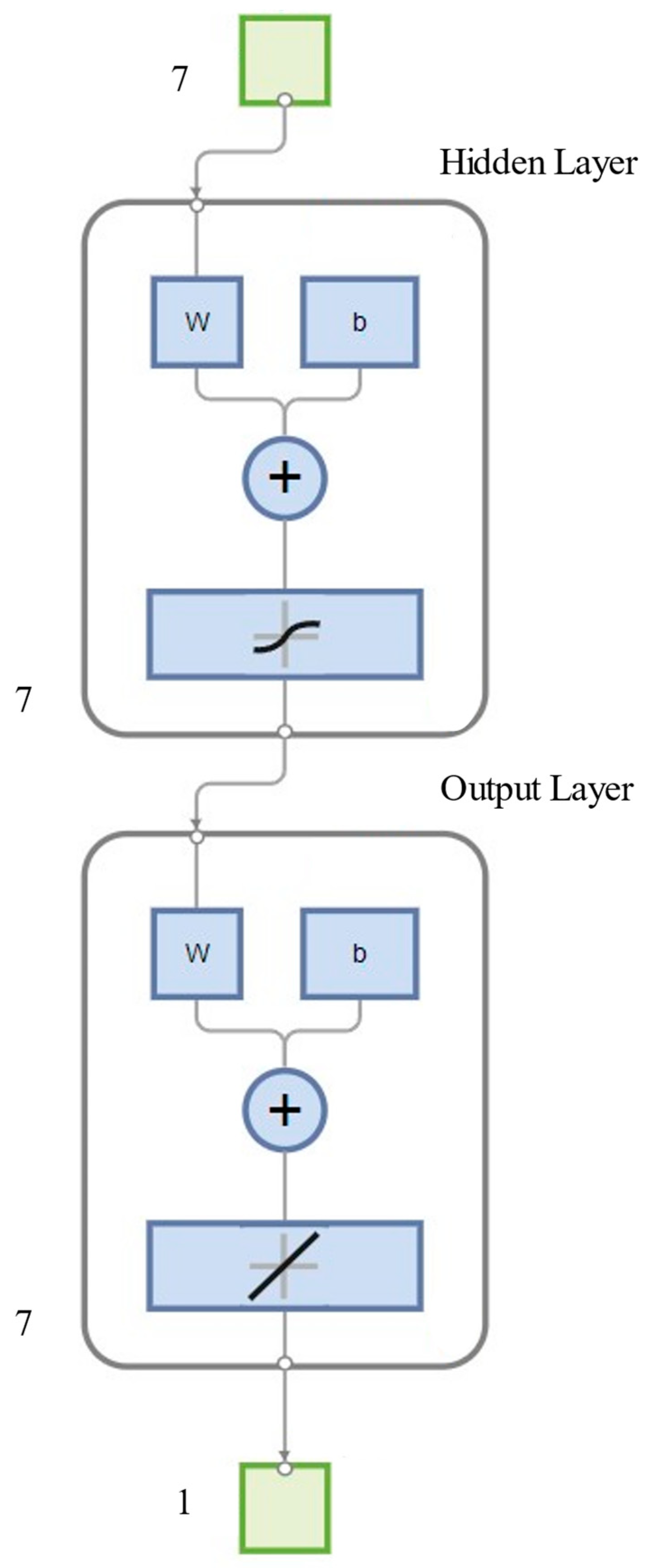
This work aims to explore the complex relationship between process parameters and mechanical performance in FFF through the integration of ANNs. This study employs a fractional Taguchi design to systematically vary seven key process parameters and generate a comprehensive dataset for model training. The primary objective is to develop an accurate ANN model capable of predicting tensile strength in FFF-produced parts. The gained knowledge should contribute to the optimization and quality assurance of 3D-printed parts. 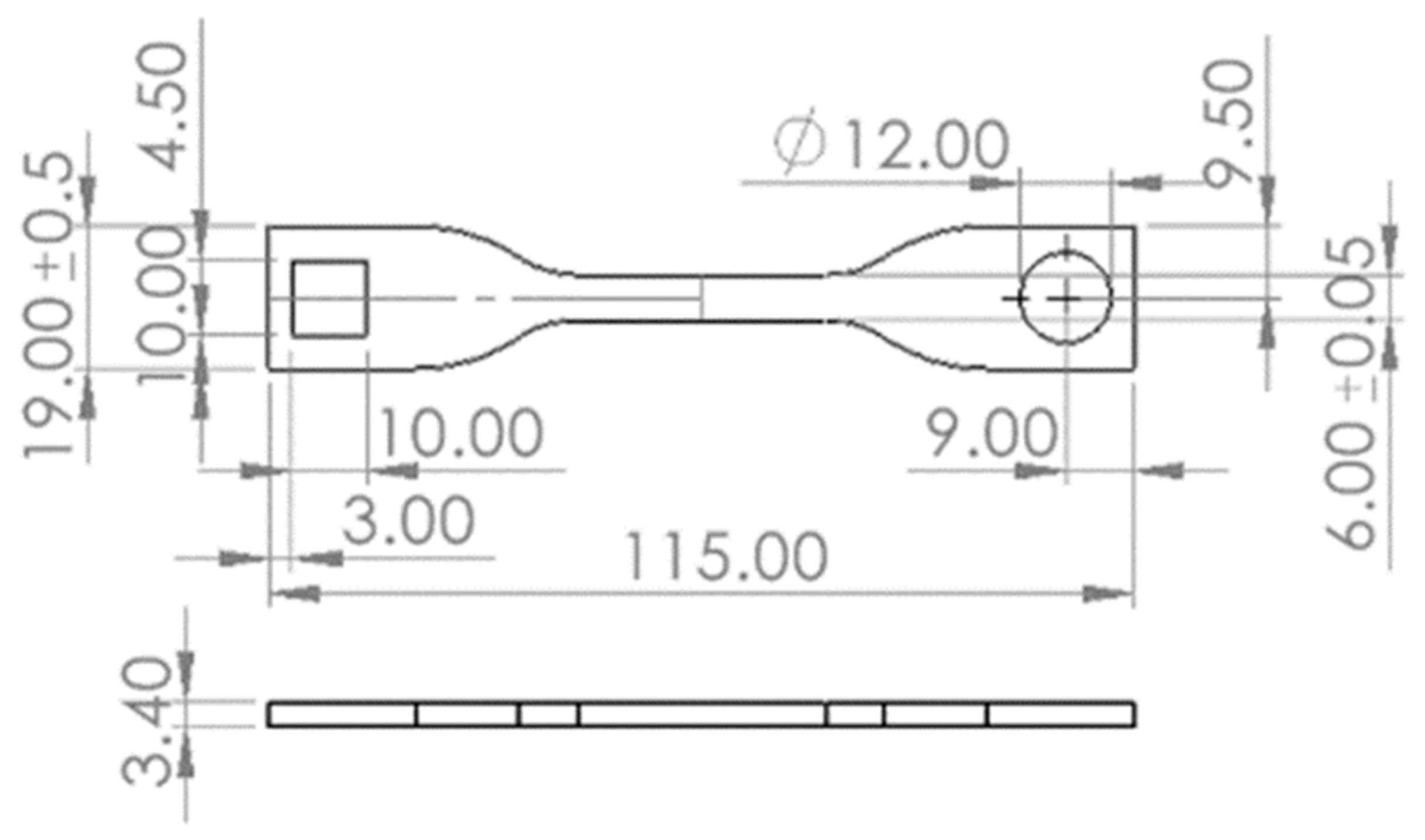This investigation is structured as follows: Section 2 discusses the materials, the benchmarks utilized in the experiments, and the manufacturing method along with the measuring procedure of the manufactured parts. 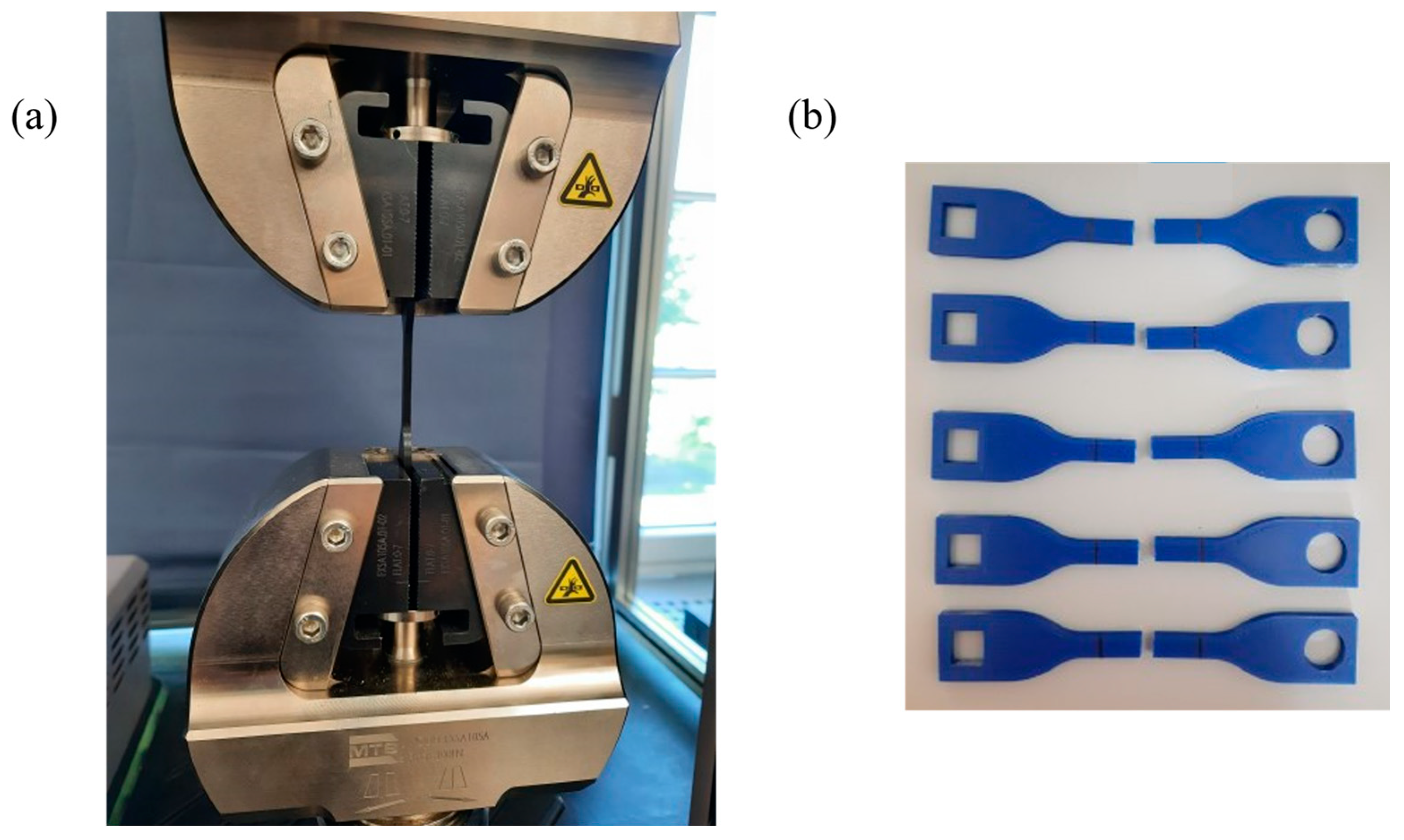Section 3 reports the mechanical tests carried out and the performance metrics for the evaluation of the ANN model. Section 4 shows the validation through additional data points to assess the prognosis. Section 6 concludes by summarizing the findings and discussing prospective future studies on the issue.

2. Materials and Methods

2.1. Printing Procedure

The FFF printer used for the experimental part is the Ultimaker S3, from Ultimaker (Utrecht, The Netherlands), equipped with a nozzle diameter of 0.4 mm. It has a building volume of 230 by 190 by 200 mm³ and a resolution of 6.9 μm in the XY direction and 2.5 μm in the Z direction [37]. The 2.85 mm diameter PLA filament from BASF Ultrafuse (Heidelberg, Germany) was used for the creation of the components [38].

For the work, a tensile specimen Type IV was designed according to the ASTM-D 638-22 standard [39] to investigate the mechanical performance of PLA parts with a thickness of 3.4 mm. A square and a hole pocket were added, as shown in Figure 1.

Seven printing parameters were defined to study the effect of varying printing process parameters on the tensile strength through Taguchi’s parametric design of experiments (DOE). A fractional Taguchi L16 was adopted where two parameters were assigned three levels of control, and the other four parameters had 4 levels of control, as shown in

Table 1. Three-dimensional printing parameters and levels from a fractional factorial DOE.

Factor	Low Level (0)	(1)	(2)	High Level (3)
A—Type of infill	Grid	Triangles	Cubic	Zig Zag
B—Infill in %	20	45	70	100
C—Print speed in mm/s	40	50	60	80
D—Layer in mm	0.1	0.2
E—Fan speed in %	50	65	80	100
F—Bed temperature in °C	50	60
G—Extrusion temperature in °C	210	220

[40]. The sixteen combinations are shown in

Table 2. L16 DOE.

Run	A	B	C	D	E	F	G
1	0	0	0	0	0	0	0
2	0	1	1	0	1	1	1
3	0	2	2	1	2	0	1
4	0	3	3	1	3	1	0
5	1	0	1	1	0	1	0
6	1	1	0	1	1	0	1
7	1	2	3	0	2	1	1
8	1	3	2	0	3	0	0
9	2	0	2	0	3	1	1
10	2	1	3	0	2	0	0
11	2	2	0	1	1	1	0
12	2	3	1	1	0	0	1
13	3	0	3	1	1	0	1
14	3	1	2	1	0	1	0
15	3	2	1	0	3	0	0
16	3	3	0	0	2	1	1

. The definitions of the printing parameter levels, such as print speed, extrusion temperature, and bed temperature, were set according to the producer material’s datasheet supplied by the printer manufacturer. Some further parameter values were set according to the literature [11,12,13,14]. The remaining process parameters were left as default for the entire experimental plan, based on their least influence on the mechanical performance. Knowing that the parts exhibit anisotropic behavior, the specimens were printed flat on the XY plane, because they have the greatest strength [41]. Since the portion in contact with the building platform is prone to warping, especially the wider corner, the brim type of adhesion was used to prevent any parts’ deformation from compromising the mechanical test results. Compared to the raft, which creates a larger support structure beneath the model, the brim has minimal interference with the test specimen, ensuring its mechanical properties during tensile testing. For each combination, 5 specimens were printed, for a total of 80 specimens.

2.2. Mechanical Test

The tensile tests were performed using a dynamometric MTS Criterion 43 machine (see Figure 2a). A gap of 70 mm was adopted according to the standard ASTM D638 [39]. The ASTM D883 [42] was consulted to choose the testing speed of 5 mm/min. Five specimens for each combination were tested. The test continued until the specimen broke. The rupture occurred within the gauge, as is shown in Figure 2b. The square and circle pockets created are not the subject of study for this paper, but it should be specified that they were placed at the clamping points, ensuring integrity throughout the test.

2.3. Artificial Neural Network Architecture

The Artificial Neural Network model was implemented using MATLAB software R2022b [43].

The ANN was trained and validated on a comprehensive dataset comprising 16 combinations with five repetitions each. The considered input parameters are outlined in Table 1. Figure 3 represents the ANN architecture. BR was used as a learning algorithm. Regularization is a widely employed technique to prevent models from becoming overly complex and overfitting the training data. Bayesian regularization, specifically implemented through the BR algorithm, proves particularly beneficial when dealing with limited or noisy data. BR allows for the expression of uncertainty in model parameters by incorporating a Bayesian framework, leading to the development of more robust and generalizable models [44].

In the context of neural networks, Bayesian regularization helps prevent overfitting by introducing a probabilistic distribution over the weights. This approach is beneficial when the dataset is small or noisy, as it allows the model to consider multiple possible weight configurations, thus expressing uncertainty in its predictions. As previously stated by the literature, it is not sensitive to overtraining and it is considered indifferent to the network’s architecture [26].

The optimal number of hidden neurons is typically between the size of the input layer and the size of the output layer. In this study, each layer has 7 hidden neurons. For the hidden layer, the Tansig activation function was used. It introduces nonlinearity into the model, which is crucial for capturing complex relationships within the data. Additionally, their bounded output range between −1 and 1 facilitates normalized outputs, which are often desirable in neural network models. The Purelin or linear function was used for the output layer, making it suitable for regression tasks where the goal is to predict continuous values.

Given the limited data points, the “Leave-One-Out” (LOO) approach, a cross-validation (CV) technique commonly utilized in machine learning and statistical modeling, was adopted [45]. In the LOO method, during each iteration of validation, the model is trained on all repetitions except one, which is reserved for verification. This systematic Leave-One-Out process provides a robust assessment of the model’s performance and generalization ability, which is especially valuable in cases of limited data. It allows for the evaluation of the network’s stability in predicting combinations of input and estimating the natural variation within a set of parameters. This process resulted in the creation and training of 80 neural networks, where 79 combinations were used for the training and 1 for the stability evaluation. In addition, 3 unseen combinations were finally used for the prediction test, to acquire the goodness of the model in predicting.

2.4. Data Preprocessing and Evaluation Metrics

To train the ANN, input and output values were normalized. The purpose was to make data comparable or to scale them in a way that simplifies analysis or training processes.

Data normalization is the process of organizing data entries to ensure uniformity across all fields and records, making information easier to find, group, and analyze.

The data were normalized in the range 0–1 according to the following formula:

$$x_n=\frac{{value}_n-{min}_i}{{max}_i-{min}_i}$$

(1)

concerning the maximum and minimum value of the i-th column.

The R-squared (R²) metric is used to evaluate the proportion of variance in the dependent variable that can be predicted from independent variables [46]. As an additional method of evaluation, the mean absolute error (MAE) measures predictive model accuracy by calculating the average absolute difference between predicted and actual values. Similarly, the mean squared error (MSE) provides insight into predictive performance by measuring the average of squared differences between predicted and actual values.

$$R^2=1-\frac{{SS}_{res}}{{SS}_{tot}}$$

(2)

$$MAE=\frac{{\sum }_{i=1}^n|y_i-x_i|}{n}$$

(3)

$$MSE=\frac{1}{n}\sum _{i=1}^n{(y_i-x_i)}^2$$

(4)

where SS_res is the residual sum of squares, SS_tot represents the total sum of squares, n is the number of observations, x is the observed value, and y is the predicted value.

A dedicated step involves assessing the prognosis quality using an independent coefficient to evaluate the approximation’s quality thoroughly. This value assesses the agreement between actual test data and the predictions made by the meta-model. The coefficient of prognosis (COP) is applied for this purpose and offers an advantage over other error measures. It is worth noting that the COP automatic scale allows for a more nuanced interpretation of the results [47].

$$COP={\left(\frac{{\sum }_{i=1}^n(x_i-\left|\overline{x}\right|)·(y_i-\left|\overline{y}\right|)}{{\sigma }_x{·\sigma }_y·(n-1)}\right)}^2$$

(5)

where $\overline{\mathrm{x}}$ and $\overline{\mathrm{y}}$ are the average values and σ_x and σ_y are the standard deviations of the samples.

3. Preliminary ANN Settings

In the field of neural model optimization, regularization techniques are crucial for improving performance and preventing overfitting. Regularization adds penalizing terms to the objective function to control the model’s complexity during training [48,49]. This approach has several benefits, including reducing variance and improving the model’s generalization to unseen data. Preliminary tests were conducted to investigate the differences between using the BR learning algorithm and the unregularized default training mode. As shown in Figure 4a, the model trained with BR showed greater stability and less discrepancy between performance with the training data and test data than the model trained without it, shown in Figure 4b.

The results indicate that the regularized model with the Bayesian approach maintains low error on both training and test data compared to the unregularized model.

4. Results

Table 3. Experimental data.

Run	UTSμ in MPa	UTSMAX in MPa	UTSMIN in MPa	σ
1	45.799	48.587	44.257	1.523
2	41.822	43.289	40.105	1.073
3	52.736	54.380	52.207	0.825
4	53.113	53.783	51.772	0.718
5	50.217	51.360	47.556	1.363
6	52.019	52.539	51.614	0.359
7	48.809	4 9.369	48.463	0.338
8	50.593	51.432	49.815	0.598
9	42.995	43.452	42.543	0.308
10	45.523	46.199	45.182	0.351
11	55.892	56.233	55.400	0.348
12	55.054	55.628	54.446	0.484
13	51.960	52.608	50.868	0.601
14	54.177	54.407	54.058	0.121
15	47.789	48.656	46.767	0.615
16	58.647	58.996	58.465	0.190

shows the average Ultimate Tensile Test (UTS_μ) values of the five repetitions, the maximum and minimum values, and the standard deviation σ for each combination. The measures exhibit very low variation, with a maximum standard deviation of 1.523.

The R² for the evaluation was not calculated since it is between two values. However, since the evaluation has the purpose of establishing the stability of the ANN when predicting already seen values, with an MAE and MSE of 0.024 and 0.002, it is possible to confirm the statement that there is a good generalization and prediction of the model (see

Table 4. ANN performance.

	Training		Evaluation
	μ	σ	μ	σ
R2 in %	97.39	0.14	-	-
MAE	0.027	0.001	0.024	0.017
MSE	0.002	0.0001	0.002	0.005
COP in %	97.40	0.14	-	-

). Furthermore, the reason behind an R² value of the training that is not exactly 100% is that the model is trained for each network on four variations of the same combination and predicts the fifth. The calculation of the COP was only possible for the training data, and the value of 97.40% demonstrates how the predicted values are close to the actual ones. The COP on the evaluation was not possible since the prediction is based only on one row.

Connection Weights to Quantify Variable Importance

Weights are fundamental parameters in ANNs, determining the effectiveness and behavior of the network. They represent the importance of connections between neurons in transmitting and transforming information. These weights determine how input is combined and weighted through the network’s layers to produce the desired output. During training, weights are adjusted to minimize errors between the predicted and desired output, ensuring accurate predictions. The connection between neural networks and their ability to process complex data enhances their effectiveness and efficiency [44,50,51].

The connection weights approach offers a straightforward evaluation of the inputs’ relative importance in model prediction. It concentrates solely on the neural network’s node connections’ weights, providing a clear and immediate view of each input’s contribution [51]. It assigns weights to input variables based on their relative importance in the network’s output. The algorithm decomposes the weights of connections between input and hidden layers, allowing for a better interpretation of results and understanding of the relationships between input and output variables.

Table 5. Input–hidden–output connection weights.

	Neuron 1	Neuron 2	Neuron 3	Neuron 4	Neuron 5	Neuron 6	Neuron 7
A	−0.395	−0.751	−0.341	−0.231	0.362	−0.151	−0.328
B	−0.414	−0.332	−0.347	−0.224	−0.330	−0.318	−0.383
C	−0.362	−0.166	−0.071	−0.187	−0.117	−0.131	−0.184
D	−0.465	−0.310	−0.330	−0.682	−0.524	−0.574	−0.570
E	−0.022	−0.036	0.377	0.624	0.279	0.521	0.521
F	−0.017	−0.024	−0.025	0.072	−0.379	0.064	−0.305
G	−0.014	−0.022	−0.023	0.013	−0.287	−0.016	−0.129
UTS	0.557	0.969	−0.357	−0.185	0.739	−0.108	−0.257

presents the weights of connections between neurons in the input, hidden, and output layers of the model.

Table 6. Connection weight approach.

Input	Relative Importance in %	Rank
A	16.9	3
B	20.2	1
C	13.3	4
D	20.1	2
E	11.4	5
F	10.0	6
G	8.1	7
Sum	100.0

evaluates the importance of different parameters in a neural network, revealing that the percentage of infill has the highest percentage contribution, at 20.2%, indicating its significant impact on the network’s output. On the other hand, the extrusion temperature has the lowest percentage contribution, at 8.1%, indicating its least impact on the network’s output [13,14,15,16].

5. ANN Validation

Three additional input combinations that differed from the initial DOE but still adhered to the input ranges, presented in

Table 7. Additional combination for ANN test.

Combination	A	B	C	D	E	F	G
C1	3	0	2	1	0	0	0
C2	3	0	2	1	3	0	0
C3	3	0	2	0	3	0	0

, were generated after completing training and evaluation. Each combination was printed with five repetitions and subjected to tensile testing.

The selection of three additional combinations was motivated by the need to test the ANN’s ability to generalize to process conditions not yet observed during training. This approach helps ensure that the model can make accurate predictions over a wide range of printing scenarios, increasing its practical utility and reliability. The assessment evaluated the ability of the ANN to predict and generalize scenarios, even when there are minor differences in printing circumstances. The three considered cases take into account the values of the layer height and fan speed that are different from those used for the training. The height of each layer has an impact on both the strength and surface quality of the printed component. Additionally, the speed of the fan can affect the cooling of the material during the printing process, which can ultimately impact the mechanical properties of the material, including its strength and ductility [11,15,16].

Table 8. Test performance.

	Test
	μ	σ
R2 in %	92.48	4.90
MAE	0.070	0.017
MSE	0.006	0.002
COP in %	99.20	2.00

displays the neural network’s ability to predict new data. The R² value is above 70%, indicating good capabilities, considering the limited number of data points used for the training part of the network.

The other performance metrics demonstrate a low prediction error, with an MAE and MSE of 0.070 and 0006, respectively. The low standard deviation values indicate a low variability and high repeatability. Finally, the results show that an excellent prognosis quality can be achieved by using the optimal meta-model, and the estimated prognosis from the COP of 99.20% indicates that the actual data closely match those of the verification dataset. Thus, the percentage difference between the data predicted by the ANN and the data obtained during the experimental campaign was calculated using the following formula:

$$Variation=\frac{{UTS}_{pred}-{UTS}_{real}}{{UTS}_{real}}·100\mathrm{\%}$$

(6)

Table 9. Experimental and predicted data from the test. Percentage variation of each predicted output from the experimental value.

Combination	UTS in MPa	UTSpred in MPa	VariationUTS in %
C1	54.945	54.325	−1.13
C2	52.671	52.054	−1.17
C3	42.554	43.643	2.56

shows that the variations are minimal, ranging from −1.17% to 2.56%, indicating a low margin of error.

6. Conclusions

In the field of additive manufacturing, FFF stands out as a transformative technology that enables the layer-by-layer construction of components without the constraints of traditional manufacturing methods. Its versatility in material usage, particularly with thermoplastics such as PLA, has attracted attention in the automotive, aerospace, and medical industries. However, the ever-increasing demand for the improved performance of 3D-printed components has spurred the integration of advanced techniques, and this study explores the pivotal role of ML in achieving this goal.

The primary objective of this work was to exploit the capabilities of ANN to predict the mechanical performance of FFF-manufactured parts. As part of a comprehensive investigation, experiments were designed using Taguchi’s parametric approach, with seven key process parameters carefully varied to study their influence on tensile strength. A fractional Taguchi L16 DOE was implemented, and the manufactured parts were tested to assess the mechanical performance of each combination.

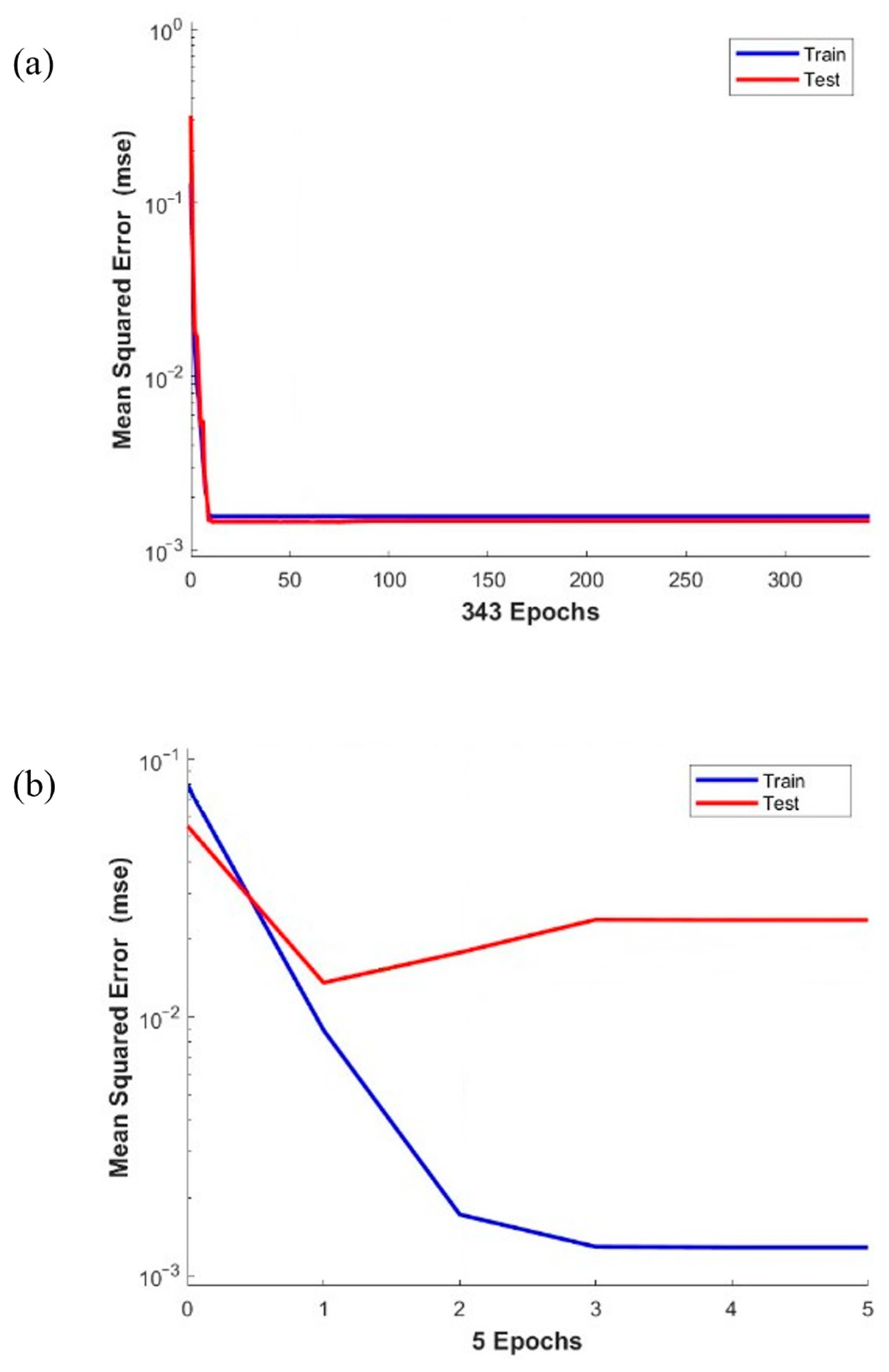
The ANN showed the ability to predict tensile strength with an R² greater than 90%. In addition, the LOO cross-validation approach provided a robust evaluation of the stability and generalization capabilities of the model with the MSE and MAE of 0.002 and 0.024.

The ANN model, trained and evaluated on the dataset, demonstrated its effectiveness in predicting unknown values. The low margin of error observed on the subsequent independent test dataset further underscored the reliability of the developed model.

The neural network with the highest R² value, equal to approximately 97%, was used to check the percentage variation between the predicted and actual values. The best model has been selected according to the score on the training and validation. The variations on the UTS remain stable within a range of −1.17% to 2.56%.

In conclusion, this study not only advances our understanding of the intricate dynamics within FFF-manufactured parts but also underscores the transformative potential of ML in optimizing and predicting mechanical performance. As industries increasingly embrace additive manufacturing, the insights gained from this work serve as a beacon to guide the path toward more efficient, reliable, and precisely engineered 3D-printed components. As demonstrated, the fusion of FFF and ML technologies drives toward a future where additive manufacturing is at the forefront of innovation and quality assurance.

Future works will include a wider range of combinations and a greater expansion of input ranges to promote a more comprehensive and complete dataset. In this way, it will be possible to increase the representativeness of the database.

References

1. D’Addona, D.M.; Raykar, S.J.; Singh, D.; Kramar, D. Multi Objective Optimization of Fused Deposition Modeling Process Parameters with Desirability Function. Procedia CIRP 2021, 99, 707–710. [Google Scholar] [CrossRef]
2. Vendittoli, V.; Polini, W.; Walter, M.S.J. An Overall Performance Index to Quantify Dimensional Accuracy and Mechanical Strength of Parts Manufactured through VAT Photopolymerization in Biodegradable and Non-Biodegradable Resin. Int. J. Adv. Manuf. Technol. 2023, 128, 5491–5502. [Google Scholar] [CrossRef]
3. ISO/ASTM 52900:2021(En); Additive Manufacturing—General Principles—Fundamentals and Vocabulary. ISO: Geneva, Switzerland. Available online: https://www.iso.org/obp/ui/#iso:std:iso-astm:52900:ed-2:v1:en:sec:A (accessed on 14 February 2024).
4. Gibson, I.; Rosen, D.W.; Stucker, B. Additive Manufacturing Technologies, 3rd ed.; Springer: Cham, Switzerland, 2015. [Google Scholar]
5. Vendittoli, V.; Polini, W.; Walter, M.S.J. Geometrical Deviations of Green Parts Due to Additive Manufacturing: A Synthetic Geometrical Performance Index. Procedia CIRP 2022, 114, 159–164. [Google Scholar] [CrossRef]
6. Abdelhamid, Z.; Habibi, M.; Kélouwani, S. The Use of Machine Learning in Process–Structure–Property Modeling for Material Extrusion Additive Manufacturing: A State-of-the-Art Review. J. Braz. Soc. Mech. Sci. Eng. 2024, 46, 70. [Google Scholar] [CrossRef]
7. Sheoran, A.J.; Kumar, H. Fused Deposition Modeling Process Parameters Optimization and Effect on Mechanical Properties and Part Quality: Review and Reflection on Present Research. Mater. Today Proc. 2020, 21, 1659–1672. [Google Scholar] [CrossRef]
8. Rajpurohit, S.R.; Dave, H.K. Effect of Process Parameters on Tensile Strength of FDM Printed PLA Part. Rapid Prototyp. J. 2018, 24, 1317–1324. [Google Scholar] [CrossRef]
9. Huynh, L.P.T.; Nguyen, H.A.; Nguyen, H.Q.; Phan, L.K.H.; Thanh, T.T. Effect of Process Parameters on Mechanical Strength of Fabricated Parts Using the Fused Deposition Modelling Method. J. Korean Soc. Precis. Eng. 2019, 36, 705–712. [Google Scholar] [CrossRef]
10. Popović, M.; Pjević, M.; Milovanović, A.; Mladenović, G.; Milošević, M. Printing Parameter Optimization of PLA Material Concerning Geometrical Accuracy and Tensile Properties Relative to FDM Process Productivity. J. Mech. Sci. Technol. 2023, 37, 697–706. [Google Scholar] [CrossRef]
11. Lee, C.-Y.; Liu, C.-Y. The Influence of Forced-Air Cooling on a 3D Printed PLA Part Manufactured by Fused Filament Fabrication. Addit. Manuf. 2019, 25, 196–203. [Google Scholar] [CrossRef]
12. Chokshi, H.; Shah, D.; Patel, K.M.; Joshi, S. Experimental Investigations of Process Parameters on Mechanical Properties for PLA during Processing in FDM. Adv. Mater. Process. Technol. 2021, 8, 696–709. [Google Scholar] [CrossRef]
13. Enemuoh, E.U.; Duginski, S.; Feyen, C.; Menta, V.G.K. Effect of Process Parameters on Energy Consumption, Physical, and Mechanical Properties of Fused Deposition Modeling. Polymers 2021, 13, 2406. [Google Scholar] [CrossRef] [PubMed]
14. Caminero, M.A.; Chacón, J.M.; Plaza, E.G.; Núñez, P.J.; Reverte, J.M.; Bécar, J.P. Additive Manufacturing of PLA-Based Composites Using Fused Filament Fabrication: Effect of Graphene Nanoplatelet Reinforcement on Mechanical Properties, Dimensional Accuracy and Texture. Polymers 2019, 11, 799. [Google Scholar] [CrossRef] [PubMed]
15. Cho, E.E.; Hein, H.H.; Lynn, Z.; Hla, S.J.; Tran, T. Investigation on Influence of Infill Pattern and Layer Thickness on Mechanical Strength of PLA Material in 3D Printing Technology. J. Eng. Sci. Res. 2019, 3, 27–37. [Google Scholar] [CrossRef]
16. Dave, H.K.; Prajapati, A.R.; Rajpurohit, S.R.; Patadiya, N.H.; Raval, H.K. Investigation on Tensile Strength and Failure Modes of FDM Printed Part Using In-House Fabricated PLA Filament. Adv. Mater. Process. Technol. 2020, 8, 576–597. [Google Scholar] [CrossRef]
17. Schmidhuber, J. Deep Learning in Neural Networks: An Overview. Neural Netw. 2015, 61, 85–117. [Google Scholar] [CrossRef]
18. Alqahtani, N.; Alam, S.; Aqeel, I.; Shuaib, M.; Khormi, I.; Khan, S.B.; Malibari, A. Deep Belief Networks (DBN) with IoT-Based Alzheimer’s Disease Detection and Classification. Appl. Sci. 2023, 13, 7833. [Google Scholar] [CrossRef]
19. Naskath, J.; Sivakamasundari, G.; Begum, A.A.S. A Study on Different Deep Learning Algorithms Used in Deep Neural Nets: MLP SOM and DBN. Wirel. Pers. Commun. 2022, 128, 2913–2936. [Google Scholar] [CrossRef] [PubMed]
20. Sheeba, A.; Bushra, S.N.; Rajarajeswari, S.; Subasini, C.A. An Efficient Starling Murmuration-Based Secure Web Service Model for Smart City Application Using DBN. Artif. Intell. Rev. 2024, 57, 72. [Google Scholar] [CrossRef]
21. Guo, D.; Song, Z.; Liu, N.; Xu, T.; Wang, X.; Zhang, Y.; Su, W.; Cheng, Y. Performance Study of Hard Rock Cantilever Roadheader Based on PCA and DBN. Rock Mech. 2024. [Google Scholar] [CrossRef]
22. Rehman, M.U.; Nizami, I.F.; Majid, M.; Ullah, F.; Hussain, I.; Chong, K.T. CN-BSRIQA: Cascaded Network—Blind Super-Resolution Image Quality Assessment. Alex. Eng. J. 2024, 91, 580–591. [Google Scholar] [CrossRef]
23. Lampinen, J.; Vehtari, A. Bayesian Approach for Neural Networks—Review and Case Studies. Neural Netw. 2001, 14, 257–274. [Google Scholar] [CrossRef]
24. Yuen, K. Recent Developments of Bayesian Model Class Selection and Applications in Civil Engineering. Struct. Saf. 2010, 32, 338–346. [Google Scholar] [CrossRef]
25. Horvitz, E.; Mulligan, D.K. Data, Privacy, and the Greater Good. Science 2015, 349, 253–255. [Google Scholar] [CrossRef] [PubMed]
26. Burden, F.R.; Winkler, D.A. Bayesian Regularization of Neural Networks. In Methods in Molecular Biology; Elsevier: Amsterdam, The Netherlands, 2008; pp. 23–42. [Google Scholar]
27. Ma, J.; Stingo, F.C.; Hobbs, B.P. Bayesian Personalized Treatment Selection Strategies That Integrate Predictive with Prognostic Determinants. Biom. J. 2019, 61, 902–917. [Google Scholar] [CrossRef] [PubMed]
28. Mekid, S.; Schlegel, T.; Aspragathos, N.A.; Teti, R. Foresight Formulation in Innovative Production, Automation and Control Systems. Foresight 2007, 9, 35–47. [Google Scholar] [CrossRef]
29. Razvi, S.A.; Feng, S.C.; Narayanan, A.; Lee, Y.-T.T.; Witherell, P. A Review of Machine Learning Applications in Additive Manufacturing. In Proceedings of the International Design Engineering Technical Conferences and Computers and Information in Engineering Conference, Washington, DC, USA, 25–28 August 2019. [Google Scholar] [CrossRef]
30. Charalampous, P.; Kladovasilakis, N.; Kostavelis, I.; Tsongas, K.; Tzetzis, D.; Tzovaras, D. Machine Learning-Based Mechanical Behavior Optimization of 3D Print Constructs Manufactured via the FFF Process. J. Mater. Eng. Perform. 2022, 31, 4697–4706. [Google Scholar] [CrossRef]
31. Nguyen, V.H.; Huynh, T.N.; Nguyen, T.-S.; Thanh, T.T. Single and Multi-Objective Optimization of Processing Parameters for Fused Deposition Modeling in 3D Printing Technology. Int. J. Automot. Mech. Eng. 2020, 17, 7542–7551. [Google Scholar] [CrossRef]
32. Jatti, V.S.; Sapre, M.S.; Jatti, A.V.; Khedkar, N.K.; Jatti, V.S. Mechanical Properties of 3D-Printed Components Using Fused Deposition Modeling: Optimization Using the Desirability Approach and Machine Learning Regressor. Appl. Syst. Innov. 2022, 5, 112. [Google Scholar] [CrossRef]
33. Manoharan, K.; Chockalingam, K.; Sasisekharan, R. Prediction of Tensile Strength in Fused Deposition Modeling Process Using Artificial Neural Network Technique. In AIP Conference Proceedings; AIP Publishing: College Park, MD, USA, 2020. [Google Scholar] [CrossRef]
34. Carrino, L.; Giorleo, G.; Polini, W.; Prisco, U. Dimensional errors in longitudinal turning based on the unified generalize mechanics of cutting approach. Part II: Machining process analysis and dimensional error estimate. Int. J. Mach. Tools Manuf. 2002, 42, 1517–1525. [Google Scholar] [CrossRef]
35. Dey, A.; Yodo, N. A Systematic Survey of FDM Process Parameter Optimization and Their Influence on Part Characteristics. J. Manuf. Mater. Process. 2019, 3, 64. [Google Scholar] [CrossRef]
36. Corrado, A.; Polini, W. Assembly design in aeronautic field: From assembly jigs to tolerance analysis. Proc. Inst. Mech. Eng. Part B J. Eng. Manuf. 2017, 14, 2652–2663. [Google Scholar] [CrossRef]
37. Ultimaker S3 Printer. Available online: https://ultimaker.com/it/3d-printers/ultimaker-s3 (accessed on 31 January 2024).
38. BASF Ultrafuse PLA 750 gr. Crea3D®. Available online: https://www.crea3d.com/en/basf/486-314-basf-ultrafuse-pla-750-gr.html (accessed on 31 January 2024).
39. ASTM D 638-22; Standard Test Method for Tensile Properties of Plastic. An American National Standard. ASTM: West Conshohocken, PA, USA. Available online: https://www.astm.org/d0638-22.html (accessed on 31 January 2024).
40. Catalogue of Taguchi Designs—Minitab. Available online: https://support.minitab.com/en-us/minitab/21/help-and-how-to/statistical-modeling/doe/supporting-topics/taguchi-designs/catalogue-of-taguchi-designs/ (accessed on 10 January 2024).
41. Afrose, M.F.; Masood, S.H.; Nikzad, M.; Iovenitti, P.G. Effects of Build Orientations on Tensile Properties of PLA Material Processed by FDM. Adv. Mater. Res. 2014, 1044–1045, 31–34. [Google Scholar] [CrossRef]
42. ASTM D 883-22; Standard Terminology Relating to Plastics. ASTM: West Conshohocken, PA, USA. Available online: https://www.astm.org/d0883-22.html (accessed on 31 January 2024).
43. MATLAB. Available online: https://www.mathworks.com/products/matlab.html (accessed on 31 January 2024).
44. Neal, R.M. Bayesian Learning for Neural Networks, 1st ed.; Springer: New York, NY, USA, 1996. [Google Scholar]
45. Bürkner, P.-C.; Gabry, J.; Vehtari, A. Efficient Leave-One-out Cross-Validation for Bayesian Non-Factorized Normal and Student-t Models. Comput. Stat. 2020, 36, 1243–1261. [Google Scholar] [CrossRef]
46. Chicco, D.; Warrens, M.J.; Jurman, G. The Coefficient of Determination R-Squared Is More Informative than SMAPE, MAE, MAPE, MSE and RMSE in Regression Analysis Evaluation. PeerJ 2021, 7, e623. [Google Scholar] [CrossRef] [PubMed]
47. Will, J.; Most, T. Metamodell of Optimized Prognosis (MoP)—An Automatic Approach for User Friendly Parameter Optimization. In Proceedings of the ANSYS Conference & 27th CADFEM Users Meeting, Leipzig, Germany, 18–20 November 2009. [Google Scholar] [CrossRef]
48. Mackay, D. Bayesian Interpolation. Neural Computat. 1992, 4, 415–447. [Google Scholar] [CrossRef]
49. Heaton, J. Ian Goodfellow, Yoshua Bengio, and Aaron Courville: Deep Learning. Genet. Program. Evolvable Mach. 2017, 19, 305–307. [Google Scholar] [CrossRef]
50. Olden, J.D.; Joy, M.K.; Death, R.G. An Accurate Comparison of Methods for Quantifying Variable Importance in Artificial Neural Networks Using Simulated Data. Ecol. Model. 2004, 178, 389–397. [Google Scholar] [CrossRef]
51. Olden, J.D.; Jackson, D.A. Illuminating the “Black Box”: A Randomization Approach for Understanding Variable Contributions in Artificial Neural Networks. Ecol. Model. 2002, 154, 135–150. [Google Scholar] [CrossRef]
Figure 1. Tensile test specimen (all dimensions in mm).
Applsci 14 03184 g001
Figure 2. (a) Setup of the tensile test machine right before starting the test procedure; (b) tensile specimens after the test.
Applsci 14 03184 g002
Figure 3. Artificial Neural Network architecture.
Applsci 14 03184 g003
Figure 4. (a) BR learning rate curves and (b) the learning curves for the non-regularized trained model.
Applsci 14 03184 g004