Finite Element Analysis for Linear Viscoelastic Materials Considering Time-Dependent Poisson’s Ratio: Variable Stiffness Method

Abstract

For linear viscoelastic materials, this paper proposes a finite element analysis method based on an integral constitutive relationship that can simultaneously consider the relaxation behavior of the elastic modulus and the creep Poisson’s ratio. Firstly, the generalized Maxwell model is employed to depict the relaxation characteristics of the elastic modulus, while the generalized Kelvin model is used to represent the creep Poisson’s ratio. Subsequently, the element relaxation stiffness matrix is established, thereby forming a convolutional finite element equation. Furthermore, the recursive calculation of the convolutional integral is derived, and the calculation steps of the finite element for viscoelasticity considering the time-dependent nature of both the elastic modulus and Poisson’s ratio are established. Finally, the accuracy of the proposed algorithm is verified through two numerical examples with linear viscoelastic material. The results indicate that the proposed variable stiffness method for the finite element analysis of linear viscoelastic materials can simultaneously consider the changes in the elastic modulus and Poisson’s ratio over time, thereby establishing a new path and idea for the more accurate simulation of viscoelastic materials’ mechanical properties. Compared with the initial strain method for linear viscoelastic materials, the variable stiffness method proposed in this paper effectively avoids the assumption of constant stress during the micro time interval, thus significantly enhancing the finite element calculation accuracy of linear viscoelastic materials. The proposed method establishes a simulation algorithm that matches existing commercial software with viscoelastic material experiments by considering the elastic modulus and Poisson’s ratio as material parameters.

1. Introduction

With the advancement of materials science, numerous polymer materials have emerged in engineering [1,2], including rubber, plastics, nylon, organic glass, textile fibers, and other industrial materials. Additionally, geological materials such as asphalt, concrete, soil, rocks, and biological materials like bones and muscles fall into this category. These materials exhibit the deformation characteristics of elastic solids and the time-dependent flow characteristics of viscous fluids during operation and use, collectively referred to as viscoelastic materials [3]. The mechanical behavior of such materials under loading depends on the magnitude of the load and varies with time. Typically, they can be regarded as linear viscoelastic materials under small strain levels.

When conducting finite element analysis on linear viscoelastic materials, there are two distinct implementation approaches based on the chosen form of constitutive relationship. One approach involves employing a differential form of constitutive relationship [4]. This approach represents the viscoelastic mechanical behavior through various combinations of force-bearing elements, such as springs and dashpots. Different combinations yield different constitutive models [5], such as the generalized Maxwell model [6], the generalized Kelvin model [7,8], and so forth. This constitutive relationship is expressed in the following form of a differential expression:

$$P\left[\sigma \left(t\right)\right]=Q\left[\epsilon \left(t\right)\right]$$

(1)

where $P$ and $Q$ represent linear differential operators with respect to time $t$, and $P=P\left(D\right)={\displaystyle \sum _{r=0}^n{p}_r\frac{d^r}{d{t}^r}}$, $Q=Q\left(D\right)={\displaystyle \sum _{r=0}^n{q}_r\frac{d^r}{d{t}^r}}$. The expanded form of the differential constitutive relationship is denoted as $\sigma +p_1\dot{\sigma }+p_2\ddot{\sigma }+\cdots =q_0\epsilon +q_1\dot{\epsilon }+q_2\ddot{\epsilon }+\cdots$, where $p_r$ and $q_r$ are material constants obtained through experiments. In different constitutive models, specific coefficients in the equation may be zero. The existing literature often employs a combination of a differential constitutive relationship and the initial strain method in developing viscoelastic finite element analysis programs, typically using the generalized Kelvin model. This model consists of a spring element and a series of Kelvin bodies (each comprising a spring and a dashpot connected in parallel). This form readily separates the total strain at any given moment into elastic strain (provided by the spring element) and viscous strain (the sum of strains from each Kelvin body). Consequently, the viscous strain can be regarded as the initial strain, enabling the use of the initial strain method employed in elastic finite element analysis for the solution. Specifically, time is discretized into a series of intervals, assuming that stress remains constant within each interval. Based on the characteristics of the generalized Kelvin model, the stress on individual spring elements and each Kelvin body connected equals the known stress within that interval. Using Kelvin’s creep compliance [9], the viscous strain of each Kelvin body under this stress is calculated and summed to obtain the total viscous strain, and this total viscous strain is treated as the initial strain. Additional forces are determined, and displacement increments caused by viscous strain during that interval are calculated. The overall analysis results are calculated step-by-step. This method maintains the stiffness matrix unchanged and equal to the initial stiffness matrix when solving the linear equation set at each interval, thus exhibiting higher computational efficiency.

However, using the initial strain method mentioned above relies on two underlying conditions: firstly, the ability to express the total strain at any given moment as the sum of elastic strain and viscous strain; secondly, the assumption that the material’s Poisson’s ratio remains constant. The first condition is only satisfied when employing structures similar to the generalized Kelvin model. This implies the necessity of knowing the creep compliance beforehand, which requires providing corresponding data through creep tests. The second condition typically applies only to some incompressible materials. However, meeting both conditions in practical engineering can be challenging due to many problems. For example, in the viscoelastic analysis of solid rocket motor propellants [10,11], which are polymer materials, relaxation tests rather than creep tests are usually conducted. These tests provide data on the relaxation modulus varying with time instead of the creep compliance [12]. Additionally, Poisson’s ratio is not constant. In such cases, the direct application of the initial strain method is not feasible.

Another approach is to employ an integral constitutive relationship [13]. This approach considers the stress–time history sum of a series of rectangular pulses over small time intervals. Utilizing the Boltzmann superposition principle, the following form of the hereditary integral is derived [14]:

$$\sigma \left(t\right)=E\left(t\right){\epsilon }_0+{\displaystyle {\int }_0^{t}E\left(t-\tau \right)\frac{d\epsilon \left(\tau \right)}{d\tau }d\tau }$$

(2)

where $\sigma \left(t\right)$ and $\epsilon \left(\tau \right)$ represent stress and strain, respectively, both of which are functions of time; $E\left(t\right)$ represents the relaxation modulus of the viscoelastic material; and ${\epsilon }_0$ represents the initial strain. Current commercial software packages such as ABAQUS 2022 and ANSYS 2023 utilize this constitutive relationship [15,16]. However, these commercial programs require the input of shear relaxation modulus $G\left(t\right)$ and bulk relaxation modulus $K\left(t\right)$, which decompose deformation at any given time into volumetric and shear components. Typically, these two relaxation moduli are assumed to follow a Prony series, with material parameters fitted from experimental data. Once these relaxation modulus expressions are determined, the remaining process is similar to the elastic finite element method. Time is discretized into a series of intervals, and numerical integration methods are used to obtain displacement and strain for each time interval. The advantage of this method lies in its generality. Regardless of the specific constitutive model used, as long as the Prony series of the relaxation modulus is obtained, the analysis can be completed following steps similar to those of traditional finite element methods. However, the drawback is apparent: forming the stiffness matrix must be repeated for each time step, resulting in high computational complexity and lower efficiency. Another drawback is the requirement for shear and bulk relaxation tests to obtain corresponding material parameters for these commercial software packages. Since these tests are operationally complex, they are rarely conducted in practical engineering. Most relaxation tests involve tension or compression [17], providing the relaxation modulus $E\left(t\right)$ over time [18,19]. Then, assuming a constant Poisson’s ratio, the bulk and shear moduli are derived from these parameters and input into the commercial software. However, this conversion process inevitably introduces additional errors. Therefore, while this method uses shear relaxation and bulk relaxation moduli, it relies solely on the elastic relaxation modulus and a constant Poisson’s ratio [20,21,22].

In summary, it is clear that whether developing custom finite element programs or using commercial software for analysis, it is commonly assumed that Poisson’s ratio remains constant throughout the entire analysis process. However, this assumption is inaccurate for many practical viscoelastic problems. For example, experimental results on Poisson’s ratio of viscoelastic materials like polymers show that it is not constant throughout the testing. It tends to increase towards 1/2 with rising temperature and prolonged loading time, while it decreases towards 1/3 with decreasing temperature and shorter loading time. Even slight variations in Poisson’s ratio can significantly impact the calculation results of mechanical properties [23,24]. Therefore, this paper aims to develop a viscoelastic finite element algorithm that can simultaneously account for the relaxation behavior of the elastic modulus and the creep Poisson’s ratio. Compared with the initial strain method, the calculation accuracy is improved by considering the time variation in Poisson’s ratio. Compared with commonly used commercial software, the required constitutive parameters are easier to obtain, thus providing a foundational algorithm for addressing such practical engineering problems.

2. Basic Principles of the Variable Stiffness Method in Finite Element Analysis of Viscoelastic Materials

2.1. The Generalized Maxwell Model for Viscoelastic Materials

Without loss of generality, the generalized Maxwell model is used to represent the relaxation properties of the elastic modulus in viscoelastic materials. Defining the elastic relaxation modulus [25,26,27]:

$$E\left(t\right)=E_{\infty }+{\displaystyle \sum _{r=1}^m{E}_r{e}^{-\frac{t}{{\tau }_r}}}$$

(3)

The creep properties of viscoelastic materials are defined using the generalized Kelvin model, and the creep Poisson’s ratio is established [28,29]:

$$\mu \left(t\right)={\mu }_0+{\displaystyle \sum _{i=1}^n{\mu }_i\left(1-e^{-\frac{t}{{\tau }_i}}\right)}$$

(4)

where $E_{\infty }$ represents the elastic coefficient of the spring element in the generalized Maxwell model, $E_r$ represents the elastic coefficient of the $r$-th Maxwell body in the generalized Maxwell model, and ${\tau }_r$ represents the relaxation time of the $r$-th Maxwell body in the generalized Maxwell model. ${\mu }_0$ represents the initial Poisson’s ratio, ${\mu }_i$ represents the elastic coefficient of the $i$-th Kelvin body in the generalized Kelvin model, and ${\tau }_i$ represents the relaxation time of the $i$-th Kelvin body in the generalized Kelvin model. $m$ and $n$ represent the number of Maxwell bodies in the generalized Maxwell model and the number of Kelvin bodies in the generalized Kelvin model, respectively. The parameters above are fitted based on data from the relaxation test for the elastic modulus and the creep test for Poisson’s ratio.

2.2. Integral Constitutive Relationship of Viscoelastic Materials

Based on the elastic relaxation modulus and creep Poisson’s ratio previously mentioned, the elastic relaxation matrix $\left[D\left(t\right)\right]$ can be defined as follows:

$$\left[D\left(t\right)\right]=\frac{E\left(t\right)}{\left(1+\mu \left(t\right)\right)\left(1-2\mu \left(t\right)\right)}\left[\begin{array}{cccccc}1-\mu \left(t\right)& \mu \left(t\right)& \mu \left(t\right)& 0& 0& 0\\ \mu \left(t\right)& 1-\mu \left(t\right)& \mu \left(t\right)& 0& 0& 0\\ \mu \left(t\right)& \mu \left(t\right)& 1-\mu \left(t\right)& 0& 0& 0\\ 0& 0& 0& \frac{1-2\mu \left(t\right)}{2}& 0& 0\\ 0& 0& 0& 0& \frac{1-2\mu \left(t\right)}{2}& 0\\ 0& 0& 0& 0& 0& \frac{1-2\mu \left(t\right)}{2}\end{array}\right]$$

(5)

With the elastic relaxation matrix above, the integral constitutive relationship of viscoelastic materials [30] can be expressed as follows:

$$\left\{\sigma \left(t\right)\right\}=D\left(t\right)\left\{{\epsilon }_0\right\}+{\displaystyle {\int }_0^t\left[D\left(t-\tau \right)\right]}\frac{\partial \left\{\epsilon \left(\tau \right)\right\}}{\partial \tau }d\tau$$

(6)

where $\left[D\left(t\right)\right]$ represents the elastic relaxation matrix at time $t$, $\left\{{\epsilon }_0\right\}$ represents the initial strain vector, and $\left\{\epsilon \left(\tau \right)\right\}$ represents the strain vector at time $\tau$. After obtaining the constitutive relationship of viscoelastic materials, similar to the finite element derivation process, the relationship between the nodal forces and nodal displacements of the element can be derived using the principle of virtual displacement:

$${\left\{P\left(t\right)\right\}}^e={\left[k\left(t\right)\right]}^e{\left\{\delta \right\}}_0^e+{\displaystyle {\int }_0^t{\left[k\left(t-\tau \right)\right]}^e\frac{\partial {\left\{\delta \left(t\right)\right\}}^e}{\partial \tau }d\tau }$$

(7)

where ${\left\{P\left(t\right)\right\}}^e$ represents the nodal force vector of the element at time t; ${\left\{\delta \right\}}_0^e$ represents the nodal displacement vector of the element at the initial moment; ${\left\{\delta \left(t\right)\right\}}^e$ represents the nodal displacement vector at time $t$; and ${\left[k\left(t\right)\right]}^e={\displaystyle \underset{v}{\int }{\left[B\right]}^T\left[D\left(t\right)\right]\left[B\right]dv}$ is the relaxation stiffness matrix of the element at time $t$, where $\left[B\right]$ represents the strain matrix.

Integrating these individual matrices yields the global relaxation stiffness matrix after obtaining the relaxation stiffness matrix for any element at a specific time. Simultaneously, by assembling the elemental load vectors into the global load vector and introducing the boundary conditions, the global equation at that time can be derived as follows:

$$K\left(t\right){\left\{\delta \right\}}_0+{\displaystyle {\int }_0^t\left[K\left(t-\tau \right)\right]\frac{\partial \left\{\delta \left(t\right)\right\}}{\partial \tau }d\tau }=\left\{P\left(t\right)\right\}$$

(8)

where $\left[K\left(t\right)\right]$ represents the global relaxation stiffness matrix at time $t$; ${\left\{\delta \right\}}_0$ represents the initial global displacement vector; $\left\{\delta \left(t\right)\right\}$ represents the global displacement vector at time $t$; and $\left\{P\left(t\right)\right\}$ represents the global load vector at time $t$.

3. Finite Element Analysis of Viscoelastic Materials Considering Time-Dependent Poisson’s Ratio

3.1. The Foundation of Convolutional Integral for Viscoelastic Materials

Numerical implementation is required to solve Equation (8) involving convolutional integrals. Here, the recursive format for convolutional integration is given. Suppose that we have the following form of a convolutional integral equation,

$${\displaystyle {\int }_{t_1}^{t}A\left(t-\tau \right)\frac{\partial y\left(\tau \right)}{\partial \tau }d\tau }=q\left(t\right)$$

(9)

where $t_1$ represents the initial moment of integration and $t$ represents the end moment of integration. In practical scenarios, $t_1=0$ can be assumed.

Let $I\left(t\right)={\displaystyle {\int }_{t_1}^{t}A\left(t-\tau \right)\frac{\partial y\left(\tau \right)}{\partial \tau }d\tau }$, and consider $t=t_{j+1}$, meaning that the equation can then be transformed to the following:

$$I\left(t_{j+1}\right)={\displaystyle {\int }_{t_1}^{t_{j+1}}A\left(t_{j+1}-\tau \right)\frac{\partial y\left(\tau \right)}{\partial \tau }d\tau }$$

(10)

If the integration time $t_1~t_{j+1}$ is discretized into a sequence of time intervals $\left[\begin{array}{ccccc}{t}_1& t_2& t_3& \begin{array}{cc}\cdots & t_j\end{array}& t_{j+1}\end{array}\right]$, then we have $j$ small time intervals, thus

$$I\left(t_{j+1}\right)={\displaystyle \sum _{k=1}^j{\displaystyle {\int }_{t_k}^{t_{k+1}}A\left(t_{j+1}-\tau \right)\frac{\partial y\left(\tau \right)}{\partial \tau }d\tau }}$$

(11)

According to the mean value theorem for integrals, the summation can be simplified as follows [31]:

$$I\left(t_{j+1}\right)={\displaystyle \sum _{k=1}^j\frac{1}{2}\left[A\left(t_{j+1}-t_{k+1}\right)+A\left(t_{j+1}-t_k\right)\right]\cdot {\displaystyle {\int }_{t_k}^{t_{k+1}}\frac{\partial y\left(\tau \right)}{\partial \tau }d\tau }}$$

(12)

Further simplification yields the following:

$$I\left(t_{j+1}\right)={\displaystyle \sum _{k=1}^j\frac{1}{2}\left[A\left(t_{j+1}-t_{k+1}\right)+A\left(t_{j+1}-t_k\right)\right]\cdot \left[y\left(t_{k+1}\right)-y\left(t_k\right)\right]}$$

(13)

Substituting the above equation into the original convolutional integral Equation (9) yields the following:

$${\displaystyle \sum _{k=1}^j\frac{1}{2}\left[A\left(t_{j+1}-t_{k+1}\right)+A\left(t_{j+1}-t_k\right)\right]\cdot \left[y\left(t_{k+1}\right)-y\left(t_k\right)\right]}=q\left(t_{j+1}\right)$$

(14)

After rearranging the above equation, the following recursive equation for solving the convolutional integral equation is derived:

$$\left\{\begin{array}{l}{\displaystyle \sum _{k=1}^{j-1}\frac{1}{2}\left[A\left(t_{j+1}-t_{k+1}\right)+A\left(t_{j+1}-t_k\right)\right]\cdot \left[y\left(t_{k+1}\right)-y\left(t_k\right)\right]}\\ +\frac{1}{2}\left[A\left(t_{j+1}-t_{j+1}\right)+A\left(t_{j+1}-t_j\right)\right]\cdot \left[y\left(t_{j+1}\right)-y\left(t_j\right)\right]=q\left(t_{j+1}\right)\\ {\displaystyle \sum _{k=1}^{j-1}\left[A\left(t_{j+1}-t_{k+1}\right)+A\left(t_{j+1}-t_k\right)\right]\cdot \left[y\left(t_{k+1}\right)-y\left(t_k\right)\right]}+\left[A\left(0\right)+A\left(t_{j+1}-t_j\right)\right]\cdot \left[y\left(t_{j+1}\right)-y\left(t_j\right)\right]=2q\left(t_{j+1}\right)\\ y\left(t_{j+1}\right)=y\left(t_j\right)+\frac{2q\left(t_{j+1}\right)-{\displaystyle \sum _{k=1}^{j-1}\left[A\left(t_{j+1}-t_{k+1}\right)+A\left(t_{j+1}-t_k\right)\right]\cdot \left[y\left(t_{k+1}\right)-y\left(t_k\right)\right]}}{A\left(0\right)+A\left(t_{j+1}-t_j\right)}\end{array}\right.$$

(15)

For the initial time point of $t=t_1$, the value of $y_1=y\left(t_1\right)$ is often determined by initial conditions. For the second time point of $t=t_2$, $y_2=y\left(t_2\right)$ is calculated using the following equation: $y_2=y_1+\frac{2q\left(t_2\right)}{A\left(0\right)+A\left(t_2-t_1\right)}$. Subsequently, starting from the third time point ($j\ge 2$), $y_{j+1}$ can be solved.

3.2. Calculation Steps of Finite Element Analysis for Viscoelastic Materials Considering Time-Dependent Poisson’s Ratio

Based on the recursive calculation provided by Equation (15) to obtain the convolutional integral, the viscoelastic finite element Equation (8) given in Section 2 can be solved. After rearrangement, the calculation steps for the variable stiffness method, which considers both the relaxation behavior of the elastic modulus and the creep Poisson’s ratio, are as follows:

(1)

Data Initialization

① Discretize the time into an array as follows: $t={\left[\begin{array}{cccccc}0,& t_1& t_2& t_3& \cdots & t_{N-1}\end{array}\right]}_{1\times N}$, where $t\left[j\right]$ represents the $j$-th element in the array, with $t\left[1\right]=0$, $t\left[2\right]=t_1$, $t\left[3\right]=t_2$, $t\left[j+1\right]=t_j$; additionally, $\Delta t_j=t\left[j+1\right]-t\left[j\right]=t_j-t_{j-1}$ is introduced.

② Determine material parameters: use experimental data and the least squares to fit the material parameters in Equations (3) and (4): $m$, $E_{\infty }$, $E_r$, ${\tau }_r$ ($r=1,2,\cdots ,m$), $n$, ${\mu }_0$, ${\mu }_i$, ${\tau }_i$ ($i=1,2,\cdots ,n$).

③ Determine the corresponding load vector for each time point: $P=\left\{\begin{array}{cccc}{P}_0& P_1& \cdots & P_{N-1}\end{array}\right\}$.

(2)

Elastic calculation at the initial time ($t=0$)

① Calculate $E\left(0\right)=E_0=E_{\infty }+{\displaystyle \sum _{r=1}^m{E}_r}$ and $\mu \left(0\right)={\mu }_0$ and derive the relaxation matrix at the initial time according to the following equation:

$$\left[D\left(0\right)\right]=\frac{E_0}{\left(1+{\mu }_0\right)\left(1-2{\mu }_0\right)}\left[\begin{array}{cccccc}1-{\mu }_0& {\mu }_0& {\mu }_0& 0& 0& 0\\ {\mu }_0& 1-{\mu }_0& {\mu }_0& 0& 0& 0\\ {\mu }_0& {\mu }_0& 1-{\mu }_0& 0& 0& 0\\ 0& 0& 0& \frac{1-2{\mu }_0}{2}& 0& 0\\ 0& 0& 0& 0& \frac{1-2{\mu }_0}{2}& 0\\ 0& 0& 0& 0& 0& \frac{1-2{\mu }_0}{2}\end{array}\right]$$

② Use the relaxation matrix obtained above and derive the initial stiffness matrix for each element at the initial time: ${\left[k\left(0\right)\right]}^e={\displaystyle \underset{v}{\int }{\left[B\right]}^T\left[D\left(0\right)\right]\left[B\right]}dv={\displaystyle {\int }_{-1}^1{\displaystyle {\int }_{-1}^1{\displaystyle {\int }_{-1}^1{\left[B\right]}^T\left[D\left(0\right)\right]\left[B\right]\cdot \left|J\right|d\xi d\eta d\varsigma }}}$.

③ Assemble the global stiffness matrix $\left[K\left(0\right)\right]$. It is important to note that the stiffness matrix at the initial time must be saved for subsequent calculations.

④ Establish the global load vector at the initial time $\left\{P\left(0\right)\right\}$, denoted as $P_0$.

⑤ Introduce any necessary boundary conditions.

⑥ Solve the following equations to obtain the displacement ${\left\{\delta \right\}}_1$ at the initial time $t\left[1\right]$.

⑦ $\left[K\left(0\right)\right]\cdot {\left\{\delta \right\}}_1=\left\{P\left(0\right)\right\}$

(3)

Calculation at the second time point, i.e., $t=t\left[2\right]=t_1$

① Calculate $\Delta t_1=t\left[2\right]-t\left[1\right]=t_1-0=t_1=t\left[2\right]$.

② Calculate $E\left(\Delta t_1\right)=E_{\infty }+{\displaystyle \sum _{r=1}^m{E}_r{e}^{-\frac{\Delta t_1}{{\tau }_r}}}$ and $\mu \left(\Delta t_1\right)={\mu }_0+{\displaystyle \sum _{i=1}^n{\mu }_i\left(1-e^{-\frac{\Delta t_1}{{\tau }_i}}\right)}$ and further construct the relaxation matrix for this time point:

$$\begin{array}{ll}\left[D\left(\Delta t_1\right)\right]& =\frac{E\left(\Delta t_1\right)}{\left(1+\mu \left(\Delta t_1\right)\right)\left(1-2\mu \left(\Delta t_1\right)\right)}\\ & \times \left[\begin{array}{cccccc}1-\mu \left(\Delta t_1\right)& \mu \left(\Delta t_1\right)& \mu \left(\Delta t_1\right)& 0& 0& 0\\ \mu \left(\Delta t_1\right)& 1-\mu \left(\Delta t_1\right)& \mu \left(\Delta t_1\right)& 0& 0& 0\\ \mu \left(\Delta t_1\right)& \mu \left(\Delta t_1\right)& 1-\mu \left(\Delta t_1\right)& 0& 0& 0\\ 0& 0& 0& \frac{1-2\mu \left(\Delta t_1\right)}{2}& 0& 0\\ 0& 0& 0& 0& \frac{1-2\mu \left(\Delta t_1\right)}{2}& 0\\ 0& 0& 0& 0& 0& \frac{1-2\mu \left(\Delta t_1\right)}{2}\end{array}\right]\end{array}$$

③ Use the relaxation matrix obtained above to formulate the stiffness matrix for each element:

$${\left[k\left(\Delta t_1\right)\right]}^e={\displaystyle \underset{v}{\int }{\left[B\right]}^T\left[D\left(\Delta t_1\right)\right]\left[B\right]}dv={\displaystyle {\int }_{-1}^1{\displaystyle {\int }_{-1}^1{\displaystyle {\int }_{-1}^1{\left[B\right]}^T\left[D\left(\Delta t_1\right)\right]\left[B\right]\cdot \left|J\right|d\xi d\eta d\varsigma }}}$$

④ Assemble the global stiffness matrix $\left[K\left(\Delta t_1\right)\right]$.

⑤ Calculate $\left[K\right]=\left[K\left(0\right)\right]+\left[K\left(\Delta t_1\right)\right]$.

⑥ Establish the global load vector for this time point $\left\{P\left(t\left[2\right]\right)\right\}$, i.e., $P_1$.

⑦ Introduce any necessary boundary conditions and solve the following equation set to determine the displacement increment $\left\{\Delta {\delta }_1\right\}$ within the first time interval; thus, $\left[K\right]\cdot \left\{\Delta {\delta }_1\right\}=2\times \left\{P\left(t\left[2\right]\right)\right\}-2\left[K\left(\Delta t_1\right)\right]\cdot {\left\{\delta \right\}}_1$.

⑧ Calculate the displacement ${\left\{\delta \right\}}_2={\left\{\delta \right\}}_1+\left\{\Delta {\delta }_1\right\}$ at this time point, i.e., the second time point, and save this displacement value.

(4)

From the third time point onwards, repeat the following steps:

$$for j=3:N$$

① Calculate $\Delta t_{j-1}=t\left[j\right]-t\left[j-1\right]$.

② Calculate $E\left(\Delta t_{j-1}\right)$, $\mu \left(\Delta t_{j-1}\right)$, $E\left(t\left[j\right]\right)$, and $\mu \left(t\left[j\right]\right)$ to establish the relaxation matrices $\left[D\left(\Delta t_{j-1}\right)\right]$ and $\left[D\left(t\left[j\right]\right)\right]$.

③ Determine the stiffness matrices ${\left[k\left(\Delta t_{j-1}\right)\right]}^e$ and ${\left[k\left(t\left[j\right]\right)\right]}^e$ for each element.

④ Assemble the global stiffness matrices $\left[K\left(\Delta t_{j-1}\right)\right]$ and $\left[K\left(t\left[j\right]\right)\right]$ corresponding to $\Delta t_{j-1}$ and $t\left[j\right]$, respectively.

⑤ Calculate $\left[K\right]=\left[K\left(0\right)\right]+\left[K\left(\Delta t_{j-1}\right)\right]$.

⑥ Calculate the additional force using the following steps:

Initialize the additional force vector $\left\{F_v\right\}$

$$for k=1:j-2$$

Calculate $\Delta t_{k+1}=t\left[j\right]-t\left[k+1\right]$ and $\Delta t_k=t\left[j\right]-t\left[k\right]$.

Calculate $E\left(\Delta t_{k+1}\right)$, $\mu \left(\Delta t_{k+1}\right)$, $E\left(\Delta t_k\right)$ and $\mu \left(\Delta t_k\right)$.

Formulate the relaxation matrices $\left[D\left(\Delta t_{k+1}\right)\right]$ and $\left[D\left(\Delta t_k\right)\right]$.

Calculate the stiffness matrices ${\left[k\left(\Delta t_{k+1}\right)\right]}^e$ and ${\left[k\left(\Delta t_k\right)\right]}^e$ for each element.

Formulate the global stiffness matrices $\left[K\left(\Delta t_{k+1}\right)\right]$ and $\left[K\left(\Delta t_k\right)\right]$ corresponding to $\Delta t_{k+1}$ and $\Delta t_k$, respectively.

Calculate ${\left[K\right]}_k=\left[K\left(\Delta t_{k+1}\right)\right]+\left[K\left(\Delta t_k\right)\right]$.

Calculate ${\left\{\Delta \delta \right\}}_k=\left\{\delta \left(t\left[k+1\right]\right)\right\}-\left\{\delta \left(t\left[k\right]\right)\right\}$.

Calculate the additional force $\left\{F_v\right\}=\left\{F_v\right\}+{\left[K\right]}_k\cdot {\left\{\Delta \delta \right\}}_k$.

end

⑦ Establish the load vector $\left\{P\left(t\left[j\right]\right)\right\}$ at the nodes for this time point.

⑧ Calculate the load vector ${\left\{\Delta P\right\}}_{j-1}=2\left\{P\left(t\left[j\right]\right)\right\}-2\left[K\left(t\left[j\right]\right)\right]\cdot {\left\{\delta \right\}}_1-\left\{F_v\right\}$ on the right-hand side of the equations for this time step.

⑨ Introduce boundary conditions, solve the following equation set, and obtain the displacement increment $\left\{\Delta {\delta }_{j-1}\right\}$ within the ($j-1$)-th time interval, yielding $\left[K\right]\cdot \left\{\Delta {\delta }_{j-1}\right\}={\left\{\Delta P\right\}}_{j-1}$.

⑩ Calculate the displacement ${\left\{\delta \right\}}_j={\left\{\delta \right\}}_{j-1}+\left\{\Delta {\delta }_{j-1}\right\}$ at this time point, i.e., $t=t\left[j\right]$, and save this displacement.

4. Verification and Discussion of the Example

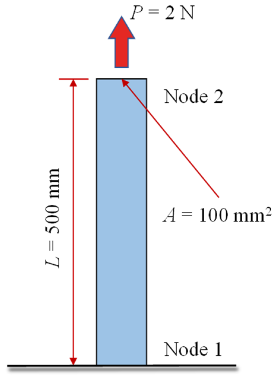
4.1. Viscoelastic Displacement of the Rod Subject to Uniaxial Tension

4.1.1. Parameter Specification

A vertical axial rod is fixed at the bottom and subjected to tensile force $P$, with material behavior described by the generalized Maxwell viscoelastic model, comprising a spring element and a Maxwell body in parallel. It is assumed that only one-dimensional elements are used. The load $P=2 \mathrm{N}$, cross-sectional area $A=100 {\mathrm{mm}}^2$, length $L=500 \mathrm{mm}$, and material parameters are $E_{\infty }=0.65 \mathrm{MPa}$ and $E_1=3 \mathrm{MPa}$. The viscosity coefficient is taken separately as ${\eta }_1=5.4 \mathrm{MPa}\cdot \mathrm{s}$, $10.8 \mathrm{MPa}\cdot \mathrm{s}$, and $21.6 \mathrm{MPa}\cdot \mathrm{s}$. The corresponding relaxation times are ${\tau }_1=1.8$, 3.6 and 7.2 s, as shown in Figure 1. The viscoelastic displacement of the rod subject to the uniaxial tension at different relaxation times is solved in this section, where the numerical results are computed using our own programmed algorithms.

4.1.2. Analytical Solution

The analytical solution can be obtained by solving the general expression of the differential constitutive equation of linear viscoelastic materials as follows:

$$P\left(D\right)\sigma =Q\left(D\right)\epsilon$$

(16)

where $P\left(D\right)={\displaystyle \sum _{k=0}^m{p}_k\frac{{\partial }^k}{\partial t^k}}$, $Q\left(D\right)={\displaystyle \sum _{k=0}^m{q}_k\frac{{\partial }^k}{\partial t^k}}$, and $D=\frac{\partial }{\partial t}$ are differential operators over time.

The generalized Maxwell model, composed of a spring element and a Maxwell element in parallel, degenerates into the traditional Poynting–Thomson model, commonly known as the H|M model (H represents Hookean spring, M represents a Maxwell element, and H|M represents a spring and a Maxwell element in parallel). Its differential constitutive equation is as follows:

$$\sigma +\frac{{\eta }_1}{E_1}\dot{\sigma }=E_{\infty }\epsilon +\left({\eta }_1+\frac{E_{\infty }{\eta }_1}{E_1}\right)\dot{\epsilon }$$

(17)

where $E_1$ and ${\eta }_1$ are the elastic and viscous coefficients of the Maxwell elements, respectively; $E_{\infty }$ is the elastic coefficient of the spring, representing the elastic modulus of the material as time approaches infinity.

Referring to the general expression (16), for the H|M model, we have the following:

$$P\left(D\right)=1+\frac{{\eta }_1}{E_1}D, Q\left(D\right)=E_{\infty }+\frac{E_1+E_{\infty }}{E_1}{\eta }_{1}D$$

(18)

Rewriting Equation (16) yields the following:

$$\sigma =\frac{Q\left(D\right)}{P\left(D\right)}\epsilon$$

(19)

It can be seen that $\frac{Q\left(D\right)}{P\left(D\right)}$ is equivalent to the elastic modulus E in elastic materials. According to the principle of elasticity–viscoelasticity correspondence, the solutions to linear viscoelastic problems are exactly the same as those of elastic problems under identical boundary conditions in Laplace space. Simply substitute E in the elastic solution with the Laplace space expression $\frac{Q\left(s\right)}{P\left(s\right)}$ corresponding to $\frac{Q\left(D\right)}{P\left(D\right)}$ in the viscoelastic constitutive equation.

Here, $Q\left(s\right)$ is the Laplace transform of $Q\left(D\right)$, and $P\left(s\right)$ is the Laplace transform of $P\left(D\right)$. For the H|M model used in the given example

$$P\left(s\right)=1+\frac{{\eta }_1}{E_1}s, Q\left(s\right)=E_{\infty }+\frac{E_1+E_{\infty }}{E_1}{\eta }_{1}s$$

(20)

Therefore,

$$\frac{Q\left(s\right)}{P\left(s\right)}=\frac{E_{\infty }+\frac{E_1+E_{\infty }}{E_1}{\eta }_{1}s}{1+\frac{{\eta }_1}{E_1}s}=E_{\infty }+\frac{E_1{\eta }_{1}s}{E_1+{\eta }_{1}s}$$

(21)

For the axial tension rod, its elastic displacement solution is $u=\frac{PL}{EA}$. According to the principle of elasticity–viscoelasticity correspondence, the linear viscoelastic displacement solution retains the same form in Laplace space. To obtain the viscoelastic displacement solution in Laplace space, simply substitute E with $\frac{Q\left(s\right)}{P\left(s\right)}$ in Equation (21), thus resulting in the expression shown below:

$$\tilde{u}\left(s\right)=\frac{PL}{sA\left(E_{\infty }+\frac{E_1{\eta }_{1}s}{E_1+{\eta }_{1}s}\right)}$$

(22)

Organize Equation (22) to obtain a form that is easy to perform inverse Laplace transform with as follows:

$$\tilde{u}\left(s\right)=\frac{PL}{A}\times \frac{E_1}{{\eta }_1\left(E_{\infty }+E_1\right)\cdot s\left[s+\frac{E_{\infty }{E}_1}{{\eta }_1\left(E_{\infty }+E_1\right)}\right]}+\frac{PL}{A}\times \frac{1}{\left(E_{\infty }+E_1\right)\cdot \left[s+\frac{E_{\infty }{E}_1}{{\eta }_1\left(E_{\infty }+E_1\right)}\right]}$$

(23)

After this arrangement, each term in Equation (23) can be identified using the Laplace transform table to find its corresponding inverse transformation form. The analytical solution of the viscoelastic problem in the time domain is then derived by applying the inverse Laplace transform to Equation (23), as shown below:

$$u\left(t\right)=\frac{PL}{A{E}_{\infty }}-\frac{PL}{A}\cdot \frac{E_1}{\left(E_{\infty }+E_1\right)E_{\infty }}{e}^{-\frac{E_{\infty }{E}_1}{{\eta }_1\left(E_{\infty }+E_1\right)}t}$$

(24)

It can be organized as follows:

$$u=\frac{PL}{A}f\left(t\right), f\left(t\right)=\frac{1}{E_{\infty }}-\frac{E_1}{E_{\infty }\left(E_1+E_{\infty }\right)}{e}^{-\frac{E_1{E}_{\infty }}{\left(E_1+E_{\infty }\right){\eta }_1}t}$$

(25)

In the given example, ${\eta }_1=10.8 \mathrm{MPa}·\mathrm{s}$; in the case of ${\tau }_1=3.6 \mathrm{s}$, we have the following:

$$\left\{\begin{array}{l}\frac{PL}{A}=\frac{1000}{100}=10\frac{\mathrm{N}}{\mathrm{mm}}\\ f\left(t\right)=\frac{1}{0.65}-\frac{3}{0.65\times 3.65}{e}^{-\frac{3\times 0.65}{3.65\times 10.8}t}=1.53846-1.264489e^{-0.049467t}\\ u\left(t\right)=10f\left(t\right)=15.3846-12.64489e^{-0.049467t}\end{array}\right.$$

(26)

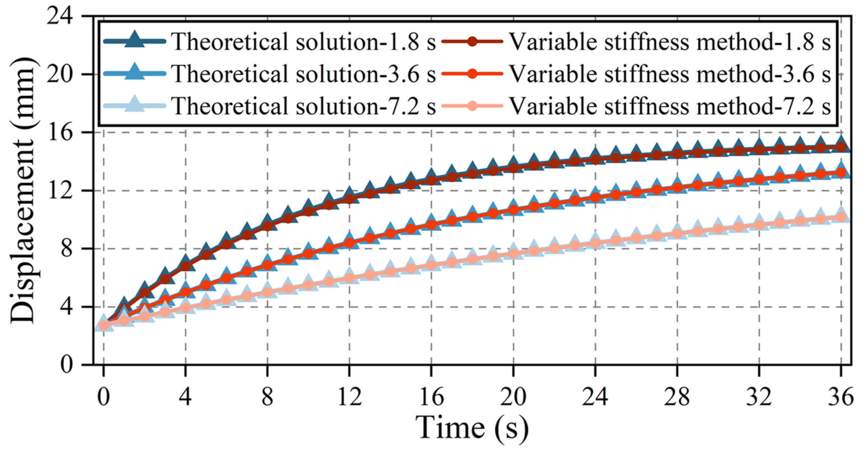
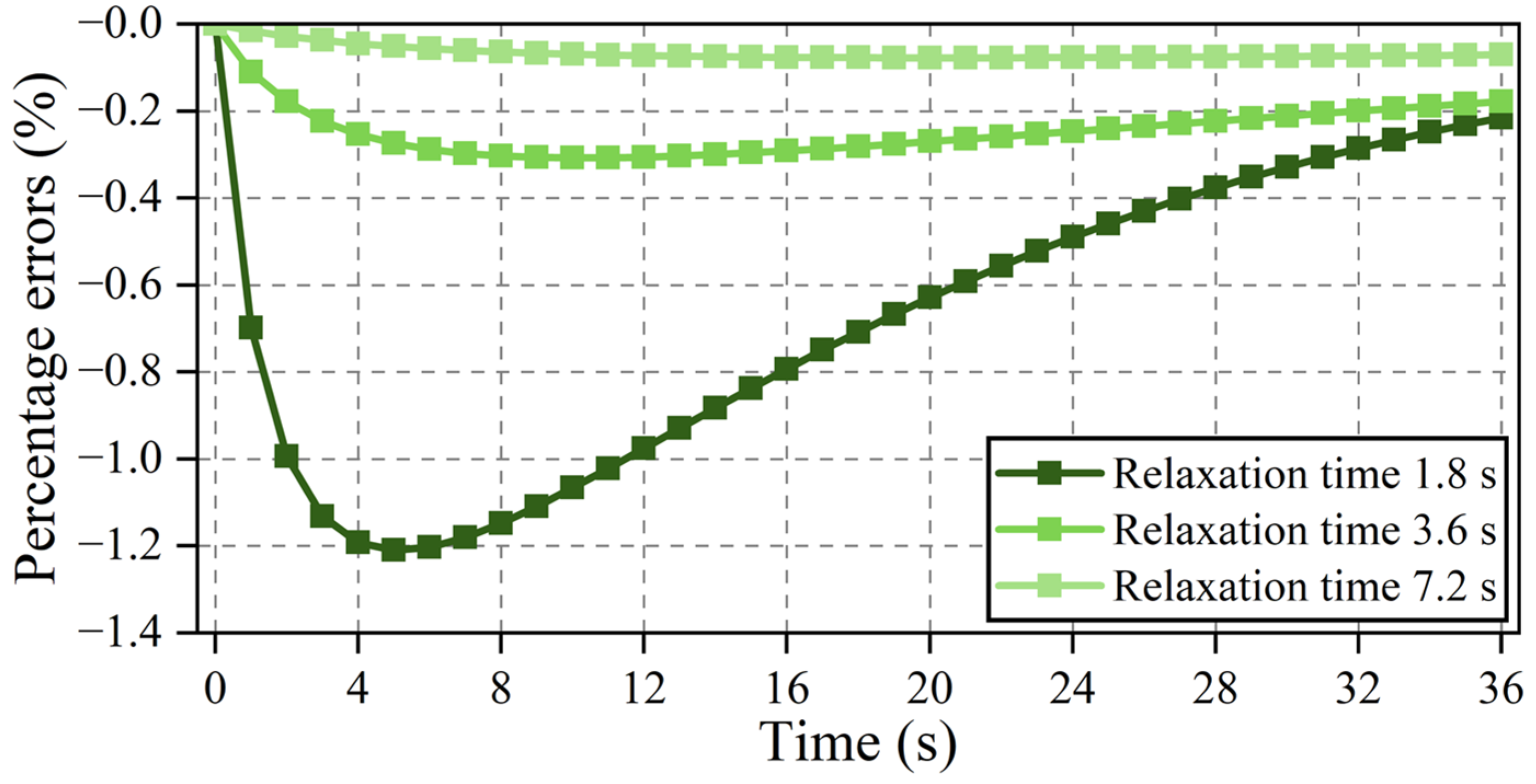
4.1.3. Comparison and Discussion of Simulation Results

Following the calculation steps previously outlined, considering the case of only one element, the viscoelastic displacements for different material parameters can be obtained. As depicted in Figure 2, the graph also includes the analytical solution obtained using Equation (25). As presented in Figure 3, the relative error of two methods under different material parameter values can be calculated using the following formula:

$$E_{error}=\frac{\left(u_{numeric}-u_{analytical}\right)\times 100}{u_{analytical}}$$

(27)

where $u_{numeric}$ is the axial tension displacement obtained by the numerical algorithm proposed in this study, $u_{analytical}$ is the analytical solution to the displacement obtained according to Equation (25), and $E_{error}$ is the relative error of the results obtained by the two methods.

From Figure 2, it is evident that in the case of using only one element, the results yielded by the algorithm proposed in this paper nearly perfectly align with the analytical solution. Under constant loading, the viscoelastic displacement of the axial rod progressively increases with time, indicating the creep properties inherent to viscoelastic materials. Analyzing the error variation depicted in Figure 3, it becomes apparent that initially, the error is minimal, followed by an increase over time, reaching a peak around the relaxation time. Subsequently, the error gradually diminishes. Throughout the process, the error consistently remains negative, indicating a slight underestimation in the calculated results compared to the analytical solution. The initial ascent and subsequent descent of the error can be attributed to the rapid change in the slope of the curve near the relaxation time, as evident from the equation for the relaxation modulus of the generalized Maxwell model. This suggests a steep slope of the curve in proximity to the relaxation time, succeeded by a more gradual change beyond this range, signifying a relatively stable relaxation modulus. In this example, for a relaxation time of 3.6 s, the stress decreases by $63.2\%$ from its initial value ($1/e$ of the initial stress), indicative of rapid attenuation. Consequently, the material parameters undergo rapid changes near the relaxation time (or within a time range of the same order of magnitude as the relaxation time). Due to the uniform time intervals used in the calculation, the error increases within this interval. However, beyond this range, as the elastic modulus changes more slowly, the error decreases. To enhance the calculation accuracy, reducing the time intervals near the relaxation time and enlarging them away from the relaxation time can be contemplated.

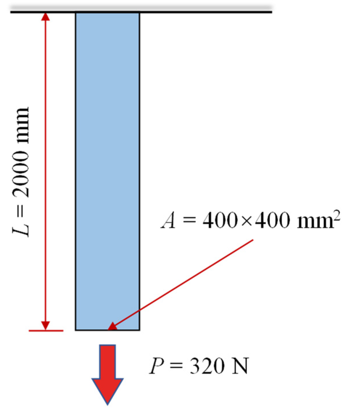
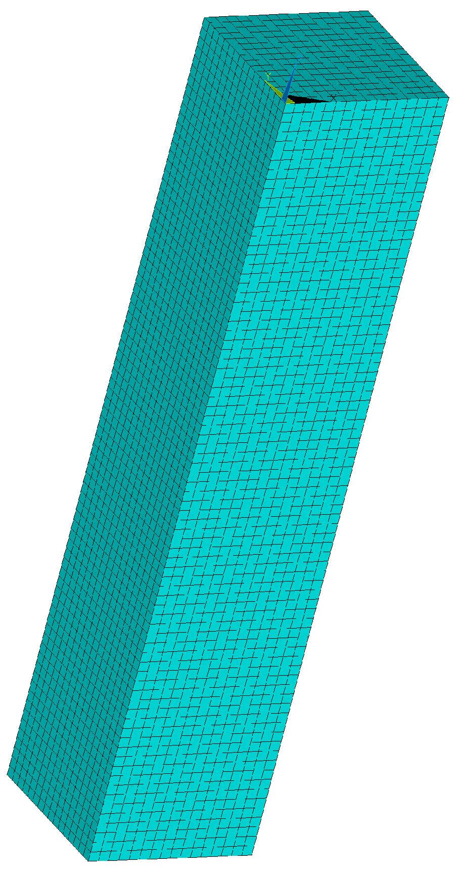
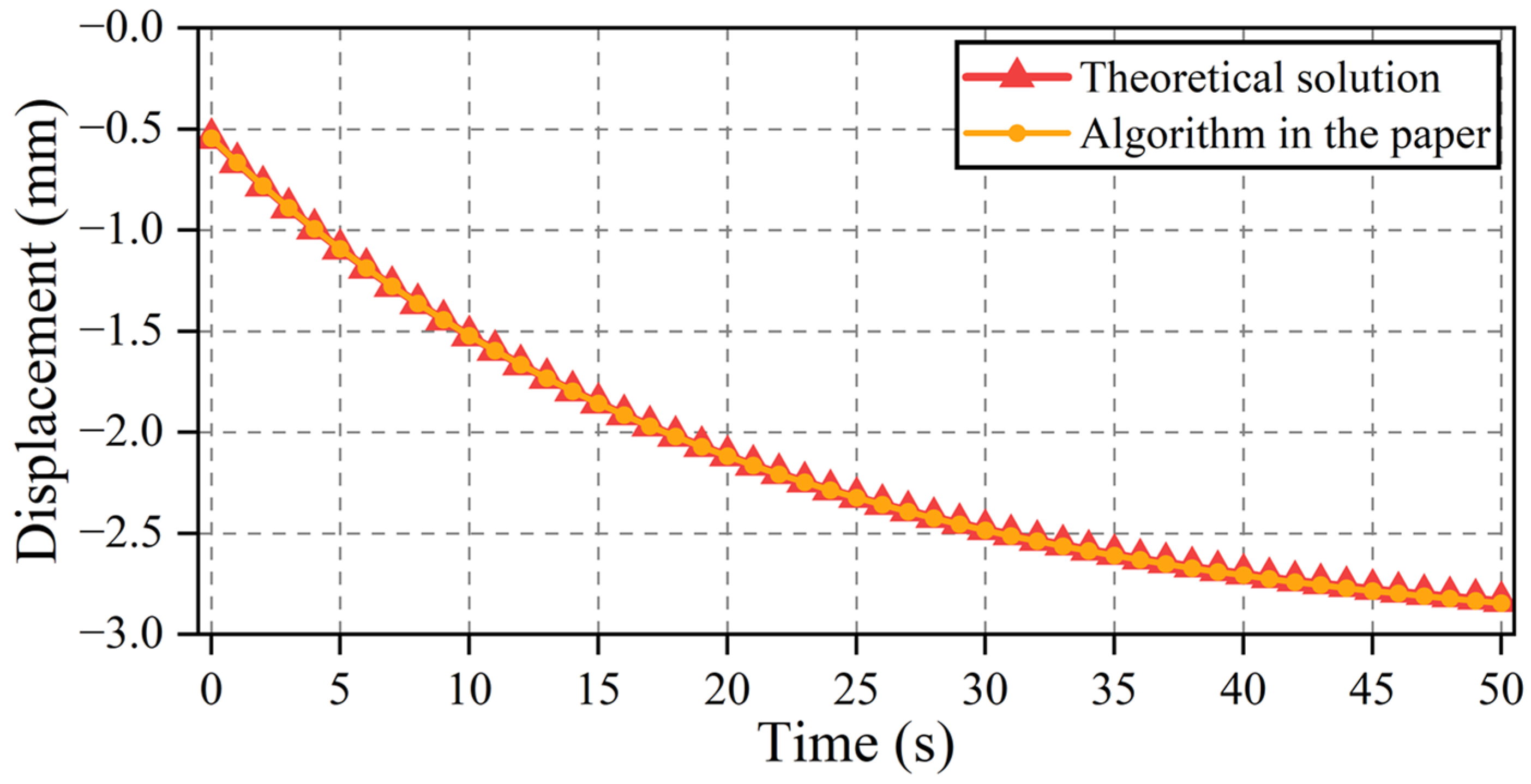
4.2. Viscoelastic Displacement of Slender Members with Equal Cross-Section under Self-Weight Effect

4.2.1. Information Detail

As depicted in Figure 4, we consider a straight rod with an equal cross-section characterized by a unit weight. $P={10}^{-6}\mathrm{N}/{\mathrm{mm}}^3$. The rod is fixed at the upper end and free at the lower end, with a length of L = 2 m (equivalent to 2000 mm) and a cross-section of $400 \mathrm{mm}\times 400 \mathrm{mm}$. The coordinate origin is denoted as O, with the z-axis extending positively upward and the y-axis oriented horizontally and positively to the right. Considering the material as linear viscoelastic and using the generalized Maxwell model to reflect the relaxation characteristics of the material’s elastic modulus as $E_{\infty }=0.65 \mathrm{MPa}$, $E_1=3 \mathrm{MPa}$. The initial elastic modulus is $E_0=3.65 \mathrm{MPa}$. Using the generalized Kelvin model to reflect the creep Poisson’s ratio of the material, where ${\mu }_0=0.34$, ${\mu }_1=0.15$, and the Poisson’s ratio at the final stable state is ${\mu }_{\infty }=0.49$. The relaxation time is 3.6 s, i.e., ${\tau }_r=\frac{{\eta }_1}{E_1}=\frac{10.8}{3}=3.6 \mathrm{s}$, ${\tau }_i={\eta }_i{\mu }_1=24\times 0.15=3.6 \mathrm{s}={\tau }_r$. The description of the material parameters is explained in the previous example.

The vertical displacement under the self-weight effect at points located at $z=0$ and $x=y=200 \mathrm{mm}$ (i.e., the corners of the bottom free end) is calculated in Figure 4.

4.2.2. Analytical Solution of Viscoelastic Displacement

According to elastic mechanics, the analytical solution for the vertical displacement of elastic materials is as follows:

$$w=\frac{P}{2E}\left[\mu \left(x^2+y^2\right)+z^2-L^2\right]$$

(28)

where E and μ are the elastic modulus and Poisson’s ratio of the material, respectively.

Using the same approach as in Section 4.1 and based on the principle of elasticity–viscoelasticity correspondence, the solution of Equation (28) in the phase space after Laplace transform can be obtained as follows:

$$w\left(s\right)=\frac{P}{2}\left[\frac{\mu \left(s\right)}{sE\left(s\right)}\left(x^2+y^2\right)+\frac{z^2-L^2}{sE\left(s\right)}\right]=w_1\left(s\right)+w_2\left(s\right)$$

(29)

and

$$w_1\left(s\right)=\frac{P}{2}\left(x^2+y^2\right)\frac{1}{s}\cdot \frac{\mu \left(s\right)}{E\left(s\right)}$$

(30)

$$w_2\left(s\right)=\frac{P}{2}\left(z^2-L^2\right)\frac{1}{sE\left(s\right)}$$

(31)

where $\mu \left(s\right)$ and $E\left(s\right)$ represent the Laplace transform of Poisson’s ratio and elastic modulus in phase space, respectively.

For this example, within the generalized Maxwell model describing the relaxation characteristics of elastic modulus, m = 1, and in the generalized Kelvin model used to describe the creep Poisson’s ratio, n = 1. Consequently, we have the following:

$$E\left(s\right)=E_{\infty }+\frac{E_{1}s}{s+\frac{1}{{\tau }_1}}$$

(32)

$$\mu \left(s\right)={\mu }_0+\frac{{\mu }_1}{{\tau }_1\left(s+\frac{1}{{\tau }_1}\right)}$$

(33)

Based on this framework, we derive the following:

$$\frac{1}{s}\cdot \frac{\mu \left(s\right)}{E\left(s\right)}=\frac{{\mu }_0}{\left(E_{\infty }+E_1\right)}\left[\frac{1}{s+\frac{E_{\infty }}{\left(E_{\infty }+E_1\right){\tau }_1}}+\frac{1}{{\tau }_1}\cdot \frac{1}{s\left(s+\frac{E_{\infty }}{\left(E_{\infty }+E_1\right){\tau }_1}\right)}\right]+\frac{{\mu }_1}{{\tau }_1\left(E_{\infty }+E_1\right)}\cdot \left[\frac{1}{s\left(s+\frac{E_{\infty }}{\left(E_{\infty }+E_1\right){\tau }_1}\right)}\right]$$

(34)

Substituting the above equation into Equation (30) and introducing $E_0=E_{\infty }+E_1$ yields the following:

$$w_1\left(s\right)=\frac{P}{2}\left(x^2+y^2\right)\frac{{\mu }_0}{E_0}\left[\frac{1}{s+\frac{E_{\infty }}{E_0{\tau }_1}}+\frac{1}{{\tau }_1}\cdot \frac{1}{s\left(s+\frac{E_{\infty }}{E_0{\tau }_1}\right)}\right]+\frac{{\mu }_1}{{\tau }_1{E}_0}\cdot \left[\frac{1}{s\left(s+\frac{E_{\infty }}{E_0{\tau }_1}\right)}\right]$$

(35)

Applying the inverse Laplace transform to Equation (35) yields the following:

$$w_1\left(t\right)=\frac{P}{2}\left(x^2+y^2\right)\cdot \frac{{\mu }_0}{E_0}\left[e^{-\frac{E_{\infty }}{E_0{\tau }_1}t}+\frac{E_0}{E_{\infty }}\left(1-e^{-\frac{E_{\infty }}{E_0{\tau }_1}t}\right)\right]+\frac{P}{2}\left(x^2+y^2\right)\cdot \frac{{\mu }_1}{E_{\infty }}\left(1-e^{-\frac{E_{\infty }}{E_0{\tau }_1}t}\right)$$

(36)

Similarly, applying the inverse Laplace transform to Equation (31) yields the following:

$$w_2\left(t\right)=\frac{P}{2}\left(z^2-L^2\right)\left(\frac{1}{E_{\infty }}-\frac{E_1}{E_{\infty }{E}_0}{e}^{-\frac{E_{\infty }}{E_0{\tau }_1}t}\right)$$

(37)

From this, the inverse Laplace transform of Equation (29) can be derived as follows:

$$w\left(t\right)=w_1\left(t\right)+w_2\left(t\right)=\frac{P}{2}\left(x^2+y^2\right)\cdot f_1\left(t\right)+\frac{P}{2}\left(z^2-L^2\right)\cdot f_2\left(t\right)$$

(38)

where

$$f_1\left(t\right)=\frac{{\mu }_{\infty }}{E_{\infty }}-\frac{\left({\mu }_0{E}_1+E_0{\mu }_1\right)}{E_0{E}_{\infty }}{e}^{-\frac{E_{\infty }}{E_0{\tau }_1}t}$$

(39)

$$f_2\left(t\right)=\frac{1}{E_{\infty }}-\frac{E_1}{E_{\infty }{E}_0}{e}^{-\frac{E_{\infty }}{E_0{\tau }_1}t}$$

(40)

In this example, the analytical solution for viscoelastic displacement, accounting for both Poisson’s ratio and elastic modulus variations over time, can be obtained by substituting the respective parameters as follows:

$$w\left(t\right)=\frac{{10}^{-6}}{2}\times 2\times {200}^2{f}_1\left(t\right)-\frac{{10}^{-6}}{2}\times 4\times {10}^6{f}_2\left(t\right)=0.04f_1\left(t\right)-2f_2\left(t\right)$$

(41)

where

$$f_1\left(t\right)=\frac{0.49}{0.65}-\frac{0.34\times 3+3.65\times 0.15}{3.65\times 0.65}{e}^{-\frac{0.65}{3.65\times 3.6}t}=0.753846-0.6607e^{-0.0494673t}$$

$$f_2\left(t\right)=\frac{1}{0.65}-\frac{3}{3.65\times 0.65}{e}^{-\frac{0.65}{3.65\times 3.6}t}=1.538461538-1.264489e^{-0.0494673t}$$

Based on the algorithm proposed in this paper, the viscoelastic displacement of the sectioned straight bar under self-weight is calculated. The time interval is set to 1 s, and the finite element mesh is partitioned, as shown in Figure 5. The calculation results of the viscoelastic displacement at the free end corner within 50 s are shown in Figure 6, where the analytical solution obtained by Equation (41) is also provided. From the calculation results, it can be observed that for the sectioned straight bar under self-weight, at the position of the free end corner, the instantaneous elastic displacement due to loading is approximately 0.5 mm. Subsequently, due to the viscous flow of the material, the viscoelastic displacement gradually increases with time, reaching 2.84 mm at 50 s, which is approximately five times the initial displacement. A comparison with the analytical solution shows that the maximum error of the algorithm proposed in this paper is about 0.3%, indicating good computational accuracy.

From the above two examples, it can be observed that when deriving analytical solutions for viscoelastic problems while leveraging the principle of elasticity–viscoelasticity correspondence, it is necessary to first obtain the analytical solution for the corresponding elastic problem. Subsequently, by applying Laplace transform, the analytical solution for the viscoelastic problem in the Laplace domain can be derived. Following this, by performing an inverse transformation, the analytical formula for the viscoelastic problem can be obtained. In many practical scenarios, however, obtaining analytical solutions for corresponding elastic problems is challenging due to the complexity of boundary conditions, geometric shapes, and loading conditions involved. Consequently, the applicability of analytical solution methods based on Laplace transform is severely limited. In contrast, the algorithm proposed in this study falls under the finite element method, which is not constrained by the conditions mentioned above. Therefore, it proves to be more suitable for addressing complex engineering problems encountered in practice.

5. Conclusions

This paper introduces a viscoelastic finite element algorithm that simultaneously considers the relaxation behavior of elastic modulus and the creep Poisson’s ratio in viscoelastic materials. The relaxation behavior of the elastic modulus is modeled using the generalized Maxwell model, while the creep Poisson’s ratio is represented using the generalized Kelvin model. Starting from the integral constitutive relationship and incorporating the principle of virtual displacement, a convolution-based variable stiffness method for solving equations is proposed. The paper also presents recursive calculations for convolution-based numerical integration. Based on this, the calculation steps of the proposed algorithm are outlined. The main conclusions of this paper can be summarized as follows:

(1)

In contrast to the initial strain method derived from the differential constitutive relationship, this algorithm can simultaneously account for the variation in the elastic modulus and Poisson’s ratio over time, thus establishing a more precise simulation pathway and a novel perspective for modeling the mechanical properties of viscoelastic materials.

(2)

Compared to the initial strain method for linear viscoelastic materials, the proposed variable stiffness method considering the time-dependent Poisson’s ratio effectively avoids the assumption of constant stress over small time intervals, thereby significantly enhancing the accuracy of the finite element calculations for linear viscoelastic materials.

(3)

Compared to the finite element method commonly used in commercial software, the proposed variable stiffness method considering the time-dependent Poisson’s ratio, with the elastic modulus and Poisson’s ratio as material parameters, establishes a simulation algorithm that aligns with experiments on viscoelastic materials.

(4)

The proposed variable stiffness method considering the time-dependent Poisson’s ratio and its calculation process effectively fits the coefficients of the Prony series for the elastic modulus and Poisson’s ratio directly based on experimental data, thereby reducing errors introduced during the transformation of material parameters when using commercial software. Future research will include additional experimental testing, convergence analysis, and investigation into computational efficiency.

References

1. Isono, Y. Viscoelastic Properties of Rubbery Materials: 1. Polymer Viscoelasticity. Nippon Gomu Kyokaishi 2018, 91, 351–357. [Google Scholar] [CrossRef]
2. Hayashi, M.; Noro, A.; Matsushita, Y. Viscoelastic properties of supramolecular soft materials with transient polymer network. J. Polym. Sci. Part B Polym. Phys. 2014, 52, 755–764. [Google Scholar] [CrossRef]
3. Findley, W.N.; Lai, J.S.; Onaran, K.; Christensen, R.M. Creep and Relaxation of Nonlinear Viscoelastic Materials With an Introduction to Linear Viscoelasticity. J. Appl. Mech. 1977, 44, 505–509. [Google Scholar] [CrossRef]
4. Ferreira, J.A.; Oliveira, P.D.; Silva, P.M.D. Reaction–diffusion in viscoelastic materials. J. Comput. Appl. Math. 2012, 236, 3783–3795. [Google Scholar] [CrossRef]
5. Chen, D.L.; Yang, P.-F.; Lai, Y.-S. A review of three-dimensional viscoelastic models with an application to viscoelasticity characterization using nanoindentation. Microelectron. Reliab. 2012, 52, 541–558. [Google Scholar] [CrossRef]
6. Cheng, Y.; Li, H.; Li, L.; Zhang, Y.; Bai, Y. Viscoelastic Properties of Asphalt Mixtures with Different Modifiers at Different Temperatures Based on Static Creep Tests. Appl. Sci. 2019, 9, 4246. [Google Scholar] [CrossRef]
7. Zhao, Y.; Ni, Y.; Zeng, W. A consistent approach for characterising asphalt concrete based on generalised Maxwell or Kelvin model. Road Mater. Pavement Des. 2014, 15, 674–690. [Google Scholar] [CrossRef]
8. Huang, W.; Wang, H.; Yin, Y.; Zhang, X.; Yuan, J. Microstructural Modeling of Rheological Mechanical Response for Asphalt Mixture Using an Image-Based Finite Element Approach. Materials 2019, 12, 2041. [Google Scholar] [CrossRef]
9. Makris, N. The frequency response function of the creep compliance. Meccanica 2019, 54, 19–31. [Google Scholar] [CrossRef]
10. Tola, C.; Nikbay, M. Solid rocket motor propellant optimization with coupled internal ballistic–structural interaction approach. J. Spacecr. Rocket. 2018, 55, 936–947. [Google Scholar] [CrossRef]
11. Yıldırım, H.; Özüpek, Ş. Structural assessment of a solid propellant rocket motor: Effects of aging and damage. Aerosp. Sci. Technol. 2011, 15, 635–641. [Google Scholar] [CrossRef]
12. Chen, X.; Xu, J.S.; Zheng, J. Solid Propellant Viscoelastic Mechanics; Beijing Institute of Technology Press: Beijing, China, 2016. [Google Scholar]
13. Cialdea, A.; Dolce, E.; Leonessa, V.; Malaspina, A. New integral representations in the linear theory of viscoelastic materials with voids. Publ. l’Inst. Math. 2014, 96, 49–65. [Google Scholar] [CrossRef]
14. Sedef, M.; Samur, E.; Basdogan, C. Real-Time Finite-Element Simulation of Linear Viscoelastic Tissue Behavior Based on Experimental Data. IEEE Comput. Graph. Appl. 2006, 26, 58–68. [Google Scholar] [CrossRef] [PubMed]
15. Zhang, X.; Liu, J. Viscoelastic creep properties and mesostructure modeling of basalt fiber-reinforced asphalt concrete. Constr. Build. Mater. 2018, 259, 119680. [Google Scholar] [CrossRef]
16. Bakhshi, B.; Arabani, M. Numerical Evaluation of Rutting in Rubberized Asphalt Mixture Using Finite Element Modeling Based on Experimental Viscoelastic Properties. J. Mater. Civ. Eng. 2018, 30, 04018088. [Google Scholar] [CrossRef]
17. Kolsky, H. An Investigation of the Mechanical Properties of Materials Very High Rates of Loading. Proc. Phys. Soc. Sect. B 1949, 62, 676–700. [Google Scholar] [CrossRef]
18. Chen, W.; Lu, F.; Cheng, M. Tension and compression tests of two polymers under quasi-static and dynamic loading. Polym. Test. 2002, 21, 113–121. [Google Scholar] [CrossRef]
19. Liu, J.; Lin, P.; Li, X.; Wang, S.-Q. Nonlinear stress relaxation behavior of ductile polymer glasses from large extension and compression. Polymer 2015, 81, 129–139. [Google Scholar] [CrossRef]
20. Tschoegl, N.W.; Knauss, W.G.; Emri, I. Poisson’s ratio in linear viscoelasticity–a critical review. Mech. Time Depend. Mater. 2002, 6, 3–51. [Google Scholar] [CrossRef]
21. Lakes, R.S.; Wineman, A. On Poisson’s ratio in linearly viscoelastic solids. J. Elast. 2006, 85, 45–63. [Google Scholar] [CrossRef]
22. Hilton, H.H. Elastic and viscoelastic Poisson’s ratios: The theoretical mechanics perspective. Mater. Sci. Appl. 2017, 8, 291–332. [Google Scholar] [CrossRef]
23. Hilton, H.H.; Yi, S. The significance of (an)isotropic viscoelastic Poisson ratio stress and time dependencies. Int. J. Solids Struct. 1998, 35, 3081–3095. [Google Scholar] [CrossRef]
24. Chyuan, S.W. Studies of poisson’s ratio variation for solid propellant grains under ignition pressure loading. Int. J. Press. Vessel. Pip. 2003, 80, 871–877. [Google Scholar] [CrossRef]
25. Angel, J.B.; Banks, J.W.; Henshaw, W.D.; Jenkinson, M.J.; Kildishev, A.V.; Kovacic, G.; Prokopeva, L.J.; Schwendeman, D.W. A high-order accurate scheme for Maxwell’s equations with a generalized dispersive material model. J. Comput. Phys. 2019, 378, 411–444. [Google Scholar] [CrossRef]
26. Babaei, B.; Davarian, A.; Pryse, K.M.; Elson, E.L.; Genin, G.M. Efficient and optimized identification of generalized Maxwell viscoelastic relaxation spectra. J. Mech. Behav. Biomed. Mater. 2016, 55, 32–41. [Google Scholar] [CrossRef]
27. Renaud, F.; Dion, J.-L.; Chevallier, G.; Tawfiq, I.; Lemaire, R. A new identification method of viscoelastic behavior: Application to the generalized Maxwell model. Mech. Syst. Signal Process. 2011, 25, 991–1010. [Google Scholar] [CrossRef]
28. Lv, H.; Ye, W.; Tan, Y.; Zhang, D. Inter-conversion of the generalized Kelvin and generalized Maxwell model parameters via a continuous spectrum method. Constr. Build. Mater. 2022, 351, 128963. [Google Scholar] [CrossRef]
29. Serra-Aguila, A.; Puigoriol-Forcada, J.; Reyes, G.; Menacho, J. Viscoelastic models revisited: Characteristics and interconversion formulas for generalized Kelvin–Voigt and Maxwell models. Acta Mech. Sin. 2019, 35, 1191–1209. [Google Scholar] [CrossRef]
30. Belfiore, L.A. Mechanical Properties of Viscoelastic Materials: Basic Concepts in Linear Viscoelasticity; Wiley-Blackwell: Hoboken, NJ, USA, 2010. [Google Scholar]
31. Silva, H.N.; Soares, J.B.; Parente, E., Jr.; Sousa, P.C. Implementation of a Viscoelastic Constitutive Model Using the Object-Oriented Programming Approach; Tech Science Press: Henderson, NV, USA, 2008. [Google Scholar]
Figure 1. Axial rod of the linear viscoelastic material.
Applsci 14 03189 g001
Figure 2. Comparison of different relaxation times.
Applsci 14 03189 g002
Figure 3. Relative error at different relaxation times.
Applsci 14 03189 g003
Figure 4. Slender members with equal cross-section and viscoelastic material.
Applsci 14 03189 g004
Figure 5. Infinite element mesh for the cross-section of straight bars.
Applsci 14 03189 g005
Figure 6. Displacement of a straight bar with equal cross-section under self-weight effect.
Applsci 14 03189 g006
Disclaimer/Publisher’s Note: The statements, opinions and data contained in all publications are solely those of the individual author(s) and contributor(s) and not of MDPI and/or the editor(s). MDPI and/or the editor(s) disclaim responsibility for any injury to people or property resulting from any ideas, methods, instructions or products referred to in the content.