
Finite Element Models to Predict the Risk of Aseptic Loosening in Cementless Femoral Stems: A Literature Review


Abstract
1. Introduction
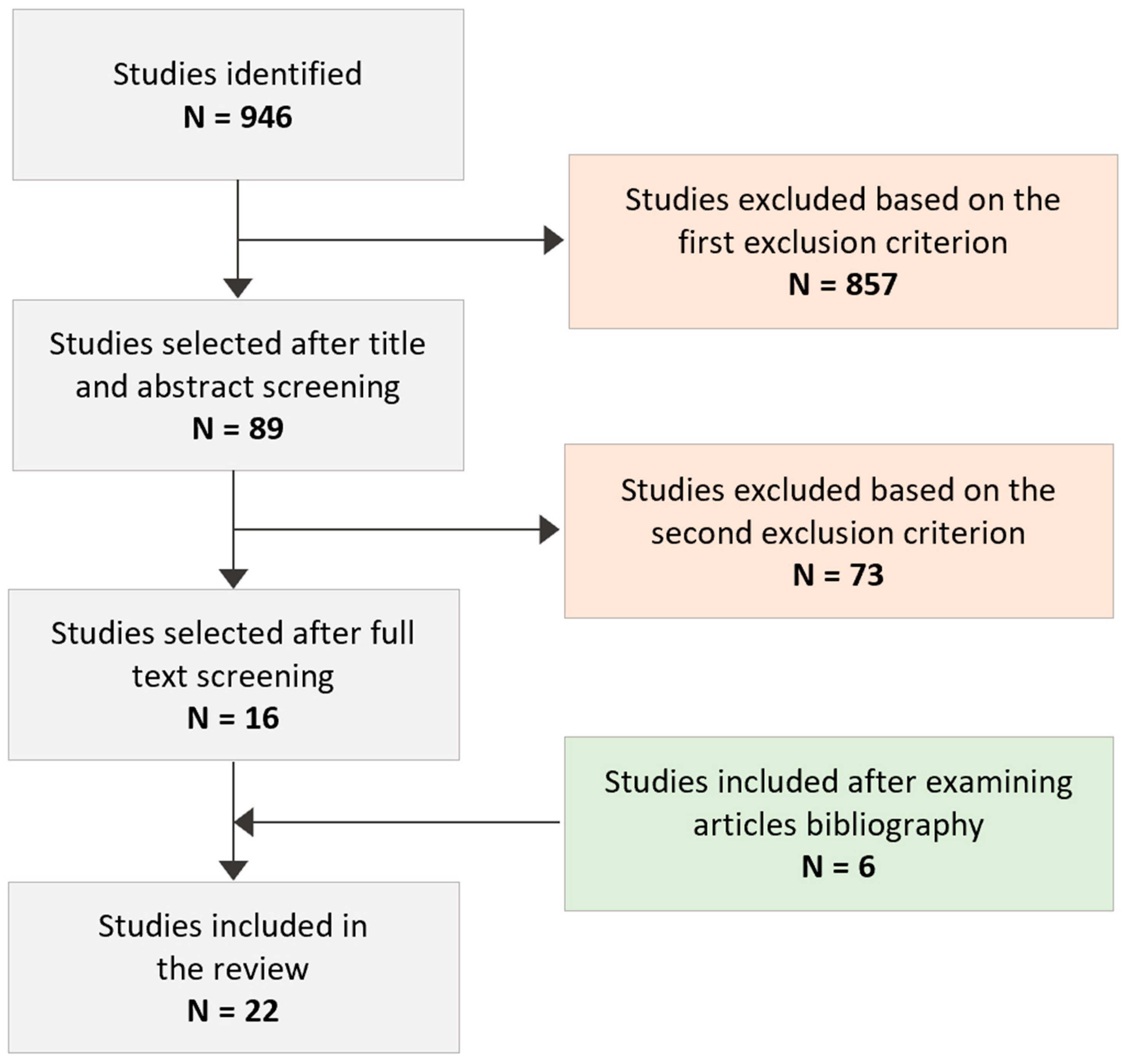
2. Studies Selection
- hip joint replacement;
- Finite Element models;
- failure modes related to aseptic loosening.
- osseointegration at the bone implant interface was not modelled;
- the implants were cemented;
- only lack of primary stability was simulated.
- characteristics of bone and implant modelling (e.g., geometry, surgical pose, material properties, and meshing);
- boundary conditions;
- bone–implant interface contact;
- quantities of interest used to predict the failure mode.

3. Search Results
3.1. Bone and Implant Features
3.1.1. Geometry
Bone
Implant
3.1.2. Bone and Implant Positioning and Initial Fitting
3.1.3. Materials
Bone
Implant
3.1.4. Mesh

| Research Paper | Geometry | Virtual Implantation and Stem Pose | Materials | Mesh | ||
|---|---|---|---|---|---|---|
| Bone | Implant | Bone | Implant | |||
| P.R. Fernandes et al. [31] 2002 | Standard human femur [54] | Tri-Lock Prosthesis of DePuy | NA | Cortical bone: E = 20 GPa; Trabecular bone: orthotropic porous material described with the homogenisation method [55,56] | Titanium (115 GPa) | Hexahedral element |
| P. Büchler et al. [40] 2003 | Three-dimensional hollow cylinder | Truncated cone | Implant placed in the central part of the bone | Cortical bone: E = 15 GPa; Trabecular bone: E = 294, 216, 150 MPa; v = 0.3 | E = 200 GPa; v = 0.3 | 8-node hexahedral elements |
| M. Viceconti et al. [29] 2004 (a) | Standard human femur | AncaFit, Cremascoli Ortho, Italy | Implanted by an expert surgeon | Cortical bone: E = 14.2 GPa; Trabecular bone: E = 69 MPa [57] | Titanium Alloy (E = 107 GPa) [57] | Three separate structured hexahedral meshes for the cortical bone, spongiosa, and implant |
| M. Viceconti et al. [42] 2004 (b) | CT scans of a composite femur [57] | AncaFit, Cremascoli Ortho, Italy | Implanted by an expert surgeon | Cortical bone: E = 14.2 GPa; Trabecular bone: E = 69 MPa [57] | Titanium Alloy (E = 107 GPa) [57] | Structured mesh with 8-node isoparametric hexahedral elements |
| P. Moreo et al. [38] 2007 | Subject-specific CT-scan dataset (middle-aged female) | Commercial design from Zweymüller (AlloPro, Baar, Switzerland) | NA | Anisotropic and heterogeneous | Stainless Steel (E = 210 GPa); Titanium (E = 84 GPa); Polyacetal (E = 20 GPa) | Hexahedral and wedge linear elements |
| X. Liu et al. [48] 2008 | 2D model of a plane | Rigid beads and a rigid bottom surface represent the prosthesis substrate | NA | Mature bone: E = 6 GPa; Immature bone: E = 1 GPa | NA | 4-node plane strain elements; three mesh densities |
| A. Lutz et al. [50] 2009 | Subject-specific CT-scan dataset | Mayo prosthesis (Zimmer, Germany) | NA | Linear elastic and isotropic, one phase continuum. Constitutive relationship between E and bone mineral density | NA | Linear tetrahedra; wedge elements for the interface layer; mesh refined gradually surrounds the implant model |
| S. Checa et al. [47] 2009 | Cube (3 × 3 × 1 mm) | Cube (3 × 3 × 1 mm) | NA | Cortical bone: Homogeneous, isotropic, and linear elastic (E = 17 GPa; v = 0.3); Immature bone: E = 1 GPa, v = 0.3 | Homogeneous, isotropic, and linear elastic (E = 100 GPa; v = 0.3) | Poroelastic elements |
| J. Folgado et al. [30] 2009 | Standard human femur [54] | Tapered-wedge shaped prosthesis (Tri-lock by DePuy; Warsaw, Indiana); Cylindrical cross-sectioned stem (AML by DePuy; Warsaw, Indiana) | Perfect initial fit between the bone and the stem was determined based on post-operative CT scans of two patients following implantation | Trabecular bone: orthotropic, porous, described with the homogenisation method [55,56] Cortical bone: E = 20 GPa | Titanium (E = 115 GPa); Co–Cr alloy (E = 230 GPa), v = 0.3 | Hexahedral meshes |
| P.K. Puthumanapully et al. [35] 2011 | Subject-specific CT-scan dataset (43-year-old male) | Commercial design from the Proxima (DePuy) | Surgical instructions | Linearly elastic, heterogeneous, and isotropic;E was assigned using BONEMAT | Titanium alloy Titanium alloy 110 GPa, linear, elastic, isotropic material | First-order tetrahedral elements (edge length: range from 0.5 to 4 mm) |
| M. Tarala et al. [28] 2011 | Subject-specific CT-scan dataset (81-year-old male) | Commercial design from VerSys Epoch FullCoat (Zimmer) | Expert surgeon guidance; in-house software within the visualised CT data (DCMTK MFC 10.8) | Isotropic; properties derived from calibrated CT data using an in-house software package | Five configurations with a layered structure varying material property composition | Linear 4-node tetrahedral elements |
| R.B. Ruben et al. [32] 2012 | Standard human femur [54] | 3D shape optimisation model based on the Tri-Lock Prosthesis of DePuy | Sensitivity to misalignments is analyzed | Bone marrow (E = 10−7 GPa), trabecular (E = 1 GPa) and cortical bone (E = 17 GPa); v = 0.3 | Titanium (E = 115 GPa; v = 0.3) | Hexahedral meshes |
| A. Andrade-Campos et al. [26] 2012 | Human femur | Commercial design from Tri-lock©/Dual-Lock© of DePuy | Follow surgical instructions; rasps are used to shape the hollow femur to fit the shape of the stem | Trabecular bone: Orthotropic, apparent material described with homogenisation [58] at microscopic level; Cortical bone: E = 20 GPa, v = 0.3 | Titanium (E = 115 GPa) | Linear hexahedral elements; remeshing technique after virtual implantation |
| A. Lutz et al. [52] 2012 | Subject-specific CT-scan dataset | Commercial design from Metha–prosthesis (Aesculap, Tuttlingen, Germany) | NA | Isotropic; power law for the constitutive relationship between Young’s modulus and bone mineral density | Titanium (E = 105 GPa) | Linear tetrahedral elements |
| M. Tarala et al. [41] 2013 | Subject-specific CT-scan dataset (81-year-old male) | VerSys Epoch FullCoat stem (Zimmer, Inc., Warsaw, IN, USA) | The stem was considered settled when a converged subsidence was achieved, meeting the criterion of incremental subsidence values being less than 1% of the total subsidence in subsequent loading periods | Elastic modulus of the bone is computed from the local ash density. Young’s Modulus ranged up to 7 GPa, 13.7 GPa, and 22.6 GPa | CoCrMo (E = 240 GPa), PEEK (E = 3.4 GPa) and Fiber mesh (E = 6.9 GPa), v = 0.3 | 4-noded tetrahedral elements |
| F. Tarlochan et al. [33] 2018 | Simplified cylindrical 3D models | Cylindrical shape with homogenous and graded porous microstructure | Interface fit introduced using a prosthesis larger than the bone inner | Cortical bone: anisotropic [59]; Trabecular bone: isotropic (E = 400 MPa) | Isotropic elastic, Ti Alloy (E = 110 GPa), v = 0.3 | Bones and calluses: 8-node poroelastic element; beads and prosthesis: 8-node solid element |
| S. Chanda et al. [27] 2020 | Subject-specific CT-scan dataset (31-year-old) | Tri-Lock (DePuy) design; One optimal stem model based on a shape optimisation study | Expert surgeon guidance | Linearly elastic, heterogeneous, and isotropic;E assigned using BONEMAT v2 | Titanium alloy (E = 110 GPa) | 10-node tetrahedra, with the interface having a relatively finer mesh (edge length ranges from 0.2 to 3.0 mm) |
| R. Ghosh et al. [36] 2020 | 3D macro-textural models of the only bone-implant interface. Three types of macro-textures based on CLS Spotorno, CORAIL and SP-CL stems | NA | Linear, elastic, homogeneous, and isotropic; (E = 500 MPa, v = 0.3) | Linear, elastic, homogeneous and isotropic material (E = 210 GPa, v = 0.3) | 8-noded hexahedral elements (edge length: maximum 1 mm) | |
| H. Mehboob et al. [37] 2020 | Subject-specific CT-scan dataset | 3D printed stem | Stems were implanted in the femur and positioned according to the ISO 7206-8: 1995 [60] | Trabecular bone: Isotropic; Cortical bone: anisotropic | CoCr alloy 230 GPa; Ti alloy 110 GPa; 30% porosity Ti 53.8 GPa; 47% porosity Ti 31.5 GPa | Quadratic tetrahedron elements (edge length: 2 mm) |
| B. Mathai and S. Gupta [51] 2022 | Subject-specific CT-scan dataset (31-year-old male); proximal femur | Commercial design from Tri-lock (DePuy); Microscale model to mimic porous surface coating | Expert surgeon guidance; virtually into the resected femur | Linearly elastic, heterogeneous and isotropic; E assigned using BONEMAT v2.0 | Titanium alloy (E = 110 GPa, v = 0.3) | 10-node tetrahedral elements; (edge length: range from 0.3 to 0.8 mm) |
| R. Ghosh et al. [39] 2022 | 3D macro-textural models of the only bone-implant interface.; two different macro-textured implant surfaces based on CORAIL and SP-CL stems | NA | Linear, elastic, homogeneous, and isotropic; (E = 500 MPa, v = 0.3) | A high-nitrogen stainless steel alloy M30NW (E = 195 Gpa), v = 0.3 | Linear elastic eight-node hexahedral elements | |
| R. Ghosh et al. [34] 2023 | Subject-specific CT-scan dataset (35-year-old female) | Implant model (CORAIL AMT hip stem) with and without macro-textures | Bone–implant assembly created using boolean operation and following surgical protocols. Orientation of the implanted femur based on the ISO 7206-4:2010 [61] | Linearly elastic, heterogeneous, and isotropic; E was assigned using BONEMAT | High-nitrogen stainless steel alloy (E = 195 GPa) | 10-noded tetra elements finer mesh at the bone-implant interface region |
3.2. Boundary Conditions
| Macroscale Models | Microscale Models | ||
|---|---|---|---|
| Research Paper | Loading Conditions | Research Paper | Loading Conditions |
| P.R. Fernandes et al. [31] J. Folgado et al. [30] R.B. Ruben et al. [32] A. Andrade-Campos et al. [26] | Peak joint forces during the stand phase of normal walking and the maximal joint load during stair climbing [66]. Muscle force considering one attachment point and hip contact forces. | X. Liu et al. [48] | Combination of 5 MPa shear and 5 MPa compressive stress, corresponding to the maximum load along the length of the stem [67] was applied to the bone part of the model. Beads and the bottom surface of the implant were fixed. |
| P. Büchler et al. [40] | Torsional loading applied to the superior part of the implant as described in [68]. | S. Checa et al. [47] | Both force- and displacement-controlled conditions were used. The bone surface is constrained. Equal pore pressure and nodal displacements on the upper and lower surfaces to approximate a repeating unit of a long implant. Under force controlled conditions, shear load, applied to the implant surface, is defined based on specific initial relative displacements (117–233 µm) between the bone and the implant resulting [69,70]. |
| M. Viceconti et al. [29] | Peak joint load during stair climbing [62] applied as hip contact force. | ||
| M. Viceconti et al. [42] | Model details are reported in [57], where stair-climbing activities are simulated considering a torsional force applied to the implant neck. | ||
| P. Moreo et al. [38] | Four different post-operation activities, including resting, were considered for the load cases. Abductor muscle and hip contact forces [62,64] were applied as two static loads. | R. Ghosh et al. [36] | Tangential displacement of 20 µm applied to the bottom surface of the implant based on [71]. Normal displacement of 20 µm is also applied to simulate press-fit conditions. Top surface of the bone is fixed. |
| A. Lutz et al. [50] A. Lutz et al. [52] | Different daily activities are considered with load values extracted from the OrthoLoad database. Load history is applied at the hip joint by discretizing the time series into static steps. Nine muscle forces are applied as static equivalent loads [72]. | R. Ghosh et al. [39] | Shear displacement (20 µm) and normal displacements (5, 10, 20, 40 µm) applied at the bottom surface of the implant to simulate micromotions at the interface and gap varying, respectively. The top surface of the bone is fixed. |
| P.K. Puthumanapully et al. [35] | Maximum loads during normal walking and stair climbing. Applied contact hip and muscle forces were extracted from [62] | ||
| M. Tarala et al. [28] | Normal walking loading conditions [64]. | ||
| M. Tarala et al. [41] | Four load increments (peak walking force, unloading, peak stair climbing force, and again unloading) are considered in each loading cycle that simulates 4 weeks in situ. | ||
| S. Chanda et al. [27] | Maximum loads during the stance phase of normal walking and stair climbing [62,64] are applied as two static load steps. Types of loads: muscles and hip contact forces. | ||
| H. Mehboob et al. [37] | Maximum loads during normal walking [63,65] applied as muscle forces and joint loads at the centre of the head stem. Post-operative conditions are considered. | ||
| R. Ghosh et al. [34] | Maximum loads during normal walking and stair climbing [63,65] applied as muscle forces and joint loads at the centre of the head stem. Post-operative conditions are considered. | ||
| Hybrid Models | |||
| Research paper | Loading Conditions for the macroscale model | Loading Conditions for the microscale model | |
| F. Tarlochan et al. [33] | Prosthesis is coaxially fixed using the interference press fit function, and the distal part of the bone is fixed. Loads are applied to the proximal end of the stem, representing the highest reaction forces of physiological body weight and muscular forces during the stance phase of the gait cycle. | External surfaces of the bone fixed. Load applied to the implant part in the longitudinal direction and defined to match the initial micromovements obtained from the micromodel (12–25 µm). Pressure that mimics interference press fit is applied at the bottom surface of the implant. | |
| B. Mathai and S. Gupta [51] | Maximum loads during the stance phase of four different daily activities are applied as muscle forces and joint forces. | Horizontal and vertical relative displacements were applied at the top bone surface. Values were obtained as average results from the macroscale model considering the four load cases. Bottom surface of the implant is fixed. | |
3.3. Bone–Implant Interface Contact
3.3.1. Direct Contact
3.3.2. Indirect Contact
3.4. Quantities of Interest
| Research Paper | Direct Contact Models |
|---|---|
| P.R. Fernandes et al. [31] | Bone remodelling was simulated by changing the bone density of the trabecular bone and contact conditions after solving an optimisation problem that considered structural compliance and total bone volume. Initial interface conditions were set to contact with a friction coefficient of 1.7 for coated surfaces and frictionless contact for uncoated surfaces. After the first iterations, relative displacement was computed for each contact node, and if the value was <50 µm, bone ingrowth was simulated by changing the contact status at that node to bonded. Once a node is set to bond, it will remain until the end. |
| P. Büchler et al. [40] | Fibrous tissue formation is based on a differential equation that includes three parameters: the rate of biological evolution v and two threshold values indicating shear strains that promote the formation, εmin, of bone tissue or fibrous tissue, εmax. The parameters were determined to match the same thickness of fibrous tissue value obtained with experimentally observed micromotion of 20 and 150 µm after 3 weeks of evolution [68]: εmin = 2.3 × 10⁻³, εmax = 8.2 × 10⁻³ and v = 5 weeks −1. The prosthesis was assumed to be in contact with the cancellous bone, with the friction coefficient set to 0.6. |
| M. Viceconti et al. [29] | The bone–implant interface was modelled with face-to-face frictional contact elements. Osseointegration was simulated using a discrete-states machine. Contact element status is set based on micromotion values dc: bonded if dc < 40 µm; gap if dc > 150 µm; frictional if 40 µm < dc > 150 µm. Bonded condition was implemented by drastically increasing the tangential contact stiffness and the normal contact stiffness. Gap status assumed fibrous tissue between bone and implant, which was modelled using the stiffness relaxation technique [75]. A contact stiffness of 15 N mm −1 was set to produce a 500 µm gap. Frictional status is modelled as an elastic frictional contact. The contact stiffness was set at 3 × 10⁴ N mm −1 to ensure peak penetration less than 1 µm. De-bonding was checked after the initial contact settings based on the stress threshold. Elements return to the friction status if: tensile stress > 0.8 MPa or shear stress > 4.9 MPa. |
| M. Viceconti et al. [42] | The bone–implant interface was modelled with face-to-face frictional contact elements. Osseointegration is simulated using a continuous and rule-based model and described for each time step and generic point at the interface with a first-order model in which the coefficient of friction µ is expressed as a function of the shear stress and micromotion. State of each contact element depends on the friction coefficients: bonded (µ > 0.32), fibrous (µ < 0.0003), and standard (0.0003 ≤ µ < 0.32). |
| J. Folgado et al. [30] | Bone remodelling was simulated as in [31]. Initial interface conditions were set to contact with a friction coefficient (0.6) for coated surfaces and frictionless contact for uncoated surfaces. After the first iteration, the relative displacement d was computed for each contact node. Two micromotion threshold values (d < 25 or < 50 µm) for the bonded contact state were analysed separately. |
| R.B. Ruben et al. [32] | Bone remodelling was simulated as in [31]. Contact elements changed status with a rule-based algorithm. Bone ingrowth occurs if all these five conditions are satisfied: relative tangential displacement < 25 µm; gap < 150 µm; tensile stress < 0.8 MPa, contact compressive stress < 7.89 MPa; shear stress below threshold values depending on the interface stiffness and related osseointegration level (e.g., shear stress should be less than 4.5 MPa when interface stiffness is zero, which corresponds to osseointegration level 1 and the initial simulated period immediately after surgery). Interface stiffness increases by one level until level 5 is reached, if all criteria are satisfied. Interface stiffness can return to zero if one of the conditions is not satisfied. |
| Research paper | Indirect contact models |
| P. Moreo et al. [38] | Bone remodelling and bone ingrowth were simulated based on the theory of continuum damage mechanics. Interface damage or interface repair was modelled by changing tissue stiffness (i.e., bounding degrees) defined based on mechanical stimuli (e.g., relative displacement at the interface). The bonded/debonded process was implemented using thin elements that connect the bone and implant with frictionless contact between the surfaces. |
| X. Liu et al. [48] | Two models were used to simulate osseointegration. In the first model, the mechano-regulatory model and diffusion analysis described in [76] were used for the differentiation of MSCs into fibroblasts, chondrocytes, and osteoblasts. The new tissue type was predicted for each element, and the effective material properties were assigned based on [76]. The second model used a modified tissue differentiation algorithm that allowed a change from immature bone to mature bone and the reverse change (bone resorption). |
| A. Lutz et al. [50] | Bone ingrowth was simulated using a linear elastic bioactive interface layer. An evolution rule for osseointegration based on normal pressure and relative motion was considered to change the tissue stiffness. |
| S. Checa et al. [47] | A lattice model that represents a space for the extracellular matrix and cells was considered for the tissue differentiation algorithm. Cells can proliferate, migrate, and differentiate according to the mechanoregulation algorithm proposed in [43], which also included the growth of the capillaries. Oxygen concentration and two mechanical stimuli, shear strain and fluid/solid velocity, were used for the differentiation of MSCs into fibroblasts, chondrocytes, and osteoblasts. Osseointegration was implemented considering a bone–implant interface layer of 1 mm thick regenerative tissue of poroelastic elements. |
| P.K. Puthumanapully et al. [35] | A uniform layer of 0.75 mm (corresponding to three layers of porous coating thickness in the Proxima implant) was created around the implant to represent the formation of granulation tissue. This layer was assumed to be fully bonded to the implant and the bone. Tissue differentiation algorithm based on the mechano-regulation theory from Carter et al. [77]. The tendency for ossification was represented by the osteogenic index ‘I’, dependent on the element stress state at each cycle. A low value of I denotes the tendency to form fibrous tissue. The index was mapped onto a range of material properties, considering an interpolated value of the Young’s modulus of the materials. Values were averaged over 10 iterations to avoid rapid changes in tissue type from one iteration to the next. Convergence was obtained after about 50 iteration or when the change in tissue type between two successive iterations in every element in the layer was less than 5%. |
| M. Tarala et al. [28] | Bone ingrowth simulated by activating spring elements based on micromotion (less than 40µm); gap value (smaller than 500 µm); local stresses (less than 25 MPa). De-bonding (spring elements deactivated) occurred when local bone stresses exceeded 25 MPa. Frictional implant–bone contact (coefficient was 0.5 or 0.88 for different materials of the stem). The spring stiffness was defined as the summation of the adjacent bone elements’ Young’s Modulus was multiplied by 1/3 of the corresponding element face area (each face had three nodes connected to it), divided by the original spring length (equal to the gap between implant and bone node). Bone remodelling was simulated only for the cases with the best bone ingrowth performance. Adaptive bone theory was used [73]. |
| A. Andrade-Campos et al. [26] | The bone–implant interface was modelled with a surface-based contact model with the penalty method (the stem is the master surface and the bone is the slave). Bone remodelling was simulated using an optimisation process that computes the evolution of volume fraction (0 void; 1 total density corresponding to cortical bone) at each point based on strain energy density values. Osseointegration was simulated by changing the stiffness of connector elements included between the bone and the stem based on a relative displacement criteria described in [31]. Osseointegration increases when the contact is achieved (normal contact force >1) and the tangential displacement is less than a threshold value. If these conditions were not verified, the initial contact conditions (contact with friction 0.3 if the surface is coated and frictionless contact for uncoated surfaces). Fully osseointegration was modelled with glued contact. De-bounded was also possible for high levels of stress (contact pressure > 0.8 MPa and shear stress > 35 MPa). |
| A. Lutz et al. [52] | An interface layer made of solid elements is considered between the bone and implant surfaces, with the initial constitutive behaviour described by the Drucker–Prager plasticity model [78]. Osseointegration is simulated considering the evolution of bone mineral density as a function of the mechanical stimuli (micromotions and strain energy density): interface stiffness, ability to carry tensile loads, and the limit until sliding occurs, which increases with ongoing mineralization. |
| M. Tarala et al. [41] | Bone ingrowth was simulated by activating spring elements with stiffness based on the ingrowth potential parameter P, which was computed based on the local micromotion stress and gap value micromotion (micromotion less than 40µm, gap value smaller than 1 mm, and local stresses less than 25 MPa). A non-linear progression of the spring stiffness was considered with P. A complete ingrowth was assumed after four loading periods (P = 1) under ideal conditions of micromotion and a gap equal to zero. Frictional implant-bone contact (coefficient 0.5). |
| F. Tarlochan et al. [33] | Microscale model of porous structures made of titanium alloy was constructed with a fixed RVE (representative volume element). The beads were initially placed inside a granulation tissue (callus) and penetrating the bone. The callus was tied to the bone and the prosthesis surface; sliding contact with a coefficient of friction of 0.4 was used between the beads and the callus and between the bone and the beads. An algorithm based on the biphasic mechano-regulation theory from Isaksson et al. 2006 [74] was used to predict tissue differentiation, including granulation tissue, fibrous tissue, intermediate bone, immature bone, cartilage, and mature bone. According to a stimulus computed using deviatoric strain and fluid flow, the material properties of the callus were updated in each element. A smoothing process was used to average the Young modulus values considered for the material properties mapping during the simulations. |
| S. Chanda et al. [27] | The bone–implant interface was modelled with large sliding surface-to-surface frictional contact elements. Bone remodelling is simulated using adaptive bone theory [13]. Bone ingrowth is simulated using contact, and spring elements (CONBIN14) are activated when the five conditions described in [32] are satisfied. Initial contact stiffness is assigned to ensure a low penetration [29] and a friction coefficient set to 0.4. Stiffness values for spring elements range between 10−6 (osseointegration level 1 at the initial post-operative condition) and 30 N/mm (the highest level of osseointegration, which corresponds to bounded contact). Spring length is defined based on the gap between two adjacent interfacial nodes. |
| R. Ghosh et al. [36] | A maximum thickness for the granulation tissue of 5 mm was assumed between the implant and the bone. The implant–tissue interface and bone–tissue interface were considered perfectly bonded. The mechano-regulatory model and diffusion analysis described in [76] were used for the differentiation of the MSCs into fibroblasts, chondrocytes, and osteoblasts. The new tissue type was predicted for each element, and the effective material properties were assigned based on [76]. The simulation was carried out for 120 iterations, which corresponded to 120 days. |
| H. Mehboob et al. [37] | Two tissue layers of 0.5 and 1 mm thick were considered to simulate the granulation tissue (callus) only at the proximal end of the stems. The callus was tied to the bone and stem surface. Ain the distal part, a surface-to surface frictional contact (0.5) was used between the stem and the bone. An algorithm based on the mechano-regulation theory from H. Isaksson et al. [74] was used to predict tissue differentiation. According to a stimulus computed using deviatoric strain, the material properties of the callus were updated for each element. A total of 16 iterations were considered for the entire simulation. |
| B. Mathai and S. Gupta [51] | An inter-bead granulation tissue of 850 µm was initially modelled with a fixed RVE only at the proximal part of the stem. The beads were assumed to penetrate the bone layer by 5 µm. Fully bonded contact was assumed between the tissue and the surfaces of the implant and bone. At the distal part, the implant-bone interface was modelled using a surface-to-surface contact with a frictional coefficient of 0.85. The tissue differentiation modelling technique presented in [36] was used. A temporal smoothing method was used to average the material properties assigned, avoiding numerical instabilities. The simulation was carried out for 60 iterations, which corresponded to 60 days. |
| R. Ghosh et al. [39] | A granulation tissue (minimum thickness of 2 mm) was assumed between the implant and the bone. The implant–tissue interface and bone-tissue interface were considered perfectly bonded. The tissue differentiation modelling technique and simulation scheme presented in [36] were used. The simulation was carried out for 120 iterations, which corresponded to 120 days. |
| R. Ghosh et al. [34] | A layer of granulation tissue (1 mm thick) was included around the proximal stem surface by Boolean subtraction operation. The implant-tissue interface and bone–tissue interface were considered perfectly bonded. In the distal part of the implant, a surface-to-surface contact was modelled between the implant and the bone with a coefficient of friction of 0.5. The tissue differentiation modelling technique presented in [36] was used. The simulation was carried out for 56 iterations, which corresponded to 56 days. |
4. Discussion
5. Conclusions
Author Contributions
Funding
Institutional Review Board Statement
Informed Consent Statement
Data Availability Statement
Acknowledgments
Conflicts of Interest
References
- Kurtz, S.M.; Ong, K.L.; Lau, E.; Widmer, M.; Maravic, M.; Gómez-Barrena, E.; de Fátima de Pina, M.; Manno, V.; Torre, M.; Walter, W.L.; et al. International Survey of Primary and Revision Total Knee Replacement. Int. Orthop. 2011, 35, 1783–1789. [Google Scholar] [CrossRef] [PubMed]
- Lübbeke, A.; Silman, A.J.; Barea, C.; Prieto-Alhambra, D.; Carr, A.J. Mapping Existing Hip and Knee Replacement Registries in Europe. Health Policy Amst. Neth. 2018, 122, 548–557. [Google Scholar] [CrossRef]
- Singh, J.A.; Yu, S.; Chen, L.; Cleveland, J.D. Rates of Total Joint Replacement in the United States: Future Projections to 2020–2040 Using the National Inpatient Sample. J. Rheumatol. 2019, 46, 1134–1140. [Google Scholar] [CrossRef]
- Rupp, M.; Lau, E.; Kurtz, S.M.; Alt, V. Projections of Primary TKA and THA in Germany from 2016 through 2040. Clin. Orthop. 2020, 478, 1622–1633. [Google Scholar] [CrossRef] [PubMed]
- Yamada, H.; Yoshihara, Y.; Henmi, O.; Morita, M.; Shiromoto, Y.; Kawano, T.; Kanaji, A.; Ando, K.; Nakagawa, M.; Kosaki, N.; et al. Cementless Total Hip Replacement: Past, Present, and Future. J. Orthop. Sci. 2009, 14, 228–241. [Google Scholar] [CrossRef]
- Toossi, N.; Adeli, B.; Timperley, A.J.; Haddad, F.S.; Maltenfort, M.; Parvizi, J. Acetabular Components in Total Hip Arthroplasty: Is There Evidence That Cementless Fixation Is Better? J. Bone Joint Surg. Am. 2013, 95, 168–174. [Google Scholar] [CrossRef]
- Report of RIPO Overall Data on Hip, Knee and Shoulder Arthroplasty in Emilia Romagna Region (Italy, 2000–2019). 2022. Available online: https://ripo.cineca.it/authzssl/pdf/Annual%20report%202019%20RIPO%20Register_v2.pdf (accessed on 13 May 2022).
- National Joint Registry 20th Annual Report 2023; Healthcare Quality Improvement Partnership Ltd.: London, UK, 2023.
- Iamthanaporn, K.; Chareancholvanich, K.; Pornrattanamaneewong, C. Revision Primary Total Hip Replacement: Causes and Risk Factors. J. Med. Assoc. Thail. Chotmaihet Thangphaet 2015, 98, 93–99. [Google Scholar]
- Sadoghi, P.; Liebensteiner, M.; Agreiter, M.; Leithner, A.; Böhler, N.; Labek, G. Revision Surgery after Total Joint Arthroplasty: A Complication-Based Analysis Using Worldwide Arthroplasty Registers. J. Arthroplast. 2013, 28, 1329–1332. [Google Scholar] [CrossRef]
- Ferguson, R.J.; Palmer, A.J.; Taylor, A.; Porter, M.L.; Malchau, H.; Glyn-Jones, S. Hip Replacement. Lancet 2018, 392, 1662–1671. [Google Scholar] [CrossRef]
- Anil, U.; Singh, V.; Schwarzkopf, R. Diagnosis and Detection of Subtle Aseptic Loosening in Total Hip Arthroplasty. J. Arthroplast. 2022, 37, 1494–1500. [Google Scholar] [CrossRef]
- Janssen, L.; Wijnands, K.A.P.; Janssen, D.; Janssen, M.W.H.E.; Morrenhof, J.W. Do Stem Design and Surgical Approach Influence Early Aseptic Loosening in Cementless THA? Clin. Orthop. 2018, 476, 1212–1220. [Google Scholar] [CrossRef] [PubMed]
- Keurentjes, J.C.; Pijls, B.G.; Van Tol, F.R.; Mentink, J.F.; Mes, S.D.; Schoones, J.W.; Fiocco, M.; Sedrakyan, A.; Nelissen, R.G. Which Implant Should We Use for Primary Total Hip Replacement? A Systematic Review and Meta-Analysis. J. Bone Joint Surg. Am. 2014, 96 (Suppl. S1), 79–97. [Google Scholar] [CrossRef] [PubMed]
- Havelin, L.I.; Espehaug, B.; Vollset, S.E.; Engesaeter, L.B. Early aseptic loosening of uncemented femoral components in primary total hip replacement. A review based on the Norwegian Arthroplasty Register. J. Bone Joint Surg. Br. 1995, 77, 11–17. [Google Scholar] [CrossRef] [PubMed]
- Wagner, M.; Schönthaler, H.; Endstrasser, F.; Dammerer, D.; Nardelli, P.; Brunner, A. Mid-Term Results After 517 Primary Total Hip Arthroplasties With a Shortened and Shoulderless Double-Taper Press-Fit Stem: High Rates of Aseptic Loosening. J. Arthroplast. 2022, 37, 97–102. [Google Scholar] [CrossRef] [PubMed]
- Hoskins, W.T.; Bingham, R.J.; Lorimer, M.; de Steiger, R.N. The Effect of Size for a Hydroxyapatite-Coated Cementless Implant on Component Revision in Total Hip Arthroplasty: An Analysis of 41,265 Stems. J. Arthroplast. 2020, 35, 1074–1078. [Google Scholar] [CrossRef]
- Graudejus, O.; Ponce Wong, R.; Varghese, N.; Wagner, S.; Morrison, B. Bridging the Gap between in Vivo and in Vitro Research: Reproducing in Vitro the Mechanical and Electrical Environment of Cells in Vivo. Front. Cell. Neurosci. 2018, 12. [Google Scholar] [CrossRef]
- AKHTAR, A. The Flaws and Human Harms of Animal Experimentation. Camb. Q. Healthc. Ethics 2015, 24, 407–419. [Google Scholar] [CrossRef] [PubMed]
- Viceconti, M.; Affatato, S.; Baleani, M.; Bordini, B.; Cristofolini, L.; Taddei, F. Pre-Clinical Validation of Joint Prostheses: A Systematic Approach. J. Mech. Behav. Biomed. Mater. 2009, 2, 120–127. [Google Scholar] [CrossRef]
- Taylor, M.; Prendergast, P.J. Four Decades of Finite Element Analysis of Orthopaedic Devices: Where Are We Now and What Are the Opportunities? J. Biomech. 2015, 48, 767–778. [Google Scholar] [CrossRef]
- Taylor, M.; Bryan, R.; Galloway, F. Accounting for Patient Variability in Finite Element Analysis of the Intact and Implanted Hip and Knee: A Review. Int. J. Numer. Methods Biomed. Eng. 2013, 29, 273–292. [Google Scholar] [CrossRef]
- Viceconti, M.; Emili, L.; Afshari, P.; Courcelles, E.; Curreli, C.; Famaey, N.; Geris, L.; Horner, M.; Jori, M.C.; Kulesza, A.; et al. Possible Contexts of Use for In Silico Trials Methodologies: A Consensus-Based Review. IEEE J. Biomed. Health Inform. 2021, 25, 3977–3982. [Google Scholar] [CrossRef]
- Favre, P.; Maquer, G.; Henderson, A.; Hertig, D.; Ciric, D.; Bischoff, J.E. In Silico Clinical Trials in the Orthopedic Device Industry: From Fantasy to Reality? Ann. Biomed. Eng. 2021, 49, 3213–3226. [Google Scholar] [CrossRef] [PubMed]
- Pankaj, P. Patient-Specific Modelling of Bone and Bone-Implant Systems: The Challenges. Int. J. Numer. Methods Biomed. Eng. 2013, 29, 233–249. [Google Scholar] [CrossRef] [PubMed]
- Andrade-Campos, A.; Ramos, A.; Simões, J.A. A Model of Bone Adaptation as a Topology Optimization Process with Contact. J. Biomed. Sci. Eng. 2012, 5, 229–244. [Google Scholar] [CrossRef]
- Chanda, S.; Mukherjee, K.; Gupta, S.; Pratihar, D.K. A Comparative Assessment of Two Designs of Hip Stem Using Rule-Based Simulation of Combined Osseointegration and Remodelling. Proc. Inst. Mech. Eng. Part H 2020, 234, 118–128. [Google Scholar] [CrossRef]
- Tarala, M.; Janssen, D.; Verdonschot, N. Balancing Incompatible Endoprosthetic Design Goals: A Combined Ingrowth and Bone Remodeling Simulation. Med. Eng. Phys. 2011, 33, 374–380. [Google Scholar] [CrossRef] [PubMed][Green Version]
- Viceconti, M.; Pancanti, A.; Dotti, M.; Traina, F.; Cristofolini, L. Effect of the Initial Implant Fitting on the Predicted Secondary Stability of a Cementless Stem. Med. Biol. Eng. Comput. 2004, 42, 222–229. [Google Scholar] [CrossRef] [PubMed]
- Folgado, J.; Fernandes, P.R.; Jacobs, C.R.; Pellegrini, V.D. Influence of Femoral Stem Geometry, Material and Extent of Porous Coating on Bone Ingrowth and Atrophy in Cementless Total Hip Arthroplasty: An Iterative Finite Element Model. Comput. Methods Biomech. Biomed. Eng. 2009, 12, 135–145. [Google Scholar] [CrossRef]
- Fernandes, P.R.; Folgado, J.; Jacobs, C.; Pellegrini, V. A Contact Model with Ingrowth Control for Bone Remodelling around Cementless Stems. J. Biomech. 2002, 35, 167–176. [Google Scholar] [CrossRef]
- Ruben, R.B.; Fernandes, P.R.; Folgado, J. On the Optimal Shape of Hip Implants. J. Biomech. 2012, 45, 239–246. [Google Scholar] [CrossRef]
- Tarlochan, F.; Mehboob, H.; Mehboob, A.; Chang, S.-H. Influence of Functionally Graded Pores on Bone Ingrowth in Cementless Hip Prosthesis: A Finite Element Study Using Mechano-Regulatory Algorithm. Biomech. Model. Mechanobiol. 2018, 17, 701–716. [Google Scholar] [CrossRef] [PubMed]
- Ghosh, R.; Hazra, A.; Chanda, S.; Chakraborty, D. Computational Assessment of Growth of Connective Tissues around Textured Hip Stem Subjected to Daily Activities after THA. Med. Biol. Eng. Comput. 2023, 61, 525–540. [Google Scholar] [CrossRef] [PubMed]
- Puthumanapully, P.K.; Browne, M. Tissue Differentiation around a Short Stemmed Metaphyseal Loading Implant Employing a Modified Mechanoregulatory Algorithm: A Finite Element Study. J. Orthop. Res. 2011, 29, 787–794. [Google Scholar] [CrossRef] [PubMed]
- Ghosh, R.; Chanda, S.; Chakraborty, D. The Influence of Macro-Textural Designs over Implant Surface on Bone on-Growth: A Computational Mechanobiology Based Study. Comput. Biol. Med. 2020, 124, 103937. [Google Scholar] [CrossRef] [PubMed]
- Mehboob, H.; Ahmad, F.; Tarlochan, F.; Mehboob, A.; Chang, S.H. A Comprehensive Analysis of Bio-Inspired Design of Femoral Stem on Primary and Secondary Stabilities Using Mechanoregulatory Algorithm. Biomech. Model. Mechanobiol. 2020, 19, 2213–2226. [Google Scholar] [CrossRef] [PubMed]
- Moreo, P.; Pérez, M.A.; García-Aznar, J.M.; Doblaré, M. Modelling the Mechanical Behaviour of Living Bony Interfaces. Comput. Methods Appl. Mech. Eng. 2007, 196, 3300–3314. [Google Scholar] [CrossRef]
- Ghosh, R.; Chanda, S.; Chakraborty, D. Influence of Sequential Opening/Closing of Interface Gaps and Texture Density on Bone Growth over Macro-Textured Implant Surfaces Using FE Based Mechanoregulatory Algorithm. Comput. Methods Biomech. Biomed. Eng. 2022, 25, 985–999. [Google Scholar] [CrossRef] [PubMed]
- Büchler, P.; Pioletti, D.P.; Rakotomanana, L.R. Biphasic Constitutive Laws for Biological Interface Evolution. Biomech. Model. Mechanobiol. 2003, 1, 239–249. [Google Scholar] [CrossRef] [PubMed]
- Tarala, M.; Janssen, D.; Verdonschot, N. Toward a Method to Simulate the Process of Bone Ingrowth in Cementless THA Using Finite Element Method. Med. Eng. Phys. 2013, 35, 543–548. [Google Scholar] [CrossRef]
- Viceconti, M.; Ricci, S.; Pancanti, A.; Cappello, A. Numerical Model to Predict the Longterm Mechanical Stability of Cementless Orthopaedic Implants. Med. Biol. Eng. Comput. 2004, 42, 747–753. [Google Scholar] [CrossRef]
- Prendergast, P. Finite Element Models in Tissue Mechanics and Orthopaedic Implant Design. Clin. Biomech. 1997, 12, 343–366. [Google Scholar] [CrossRef] [PubMed]
- Ghosh, R.; Chanda, S.; Chakraborty, D. Application of Finite Element Analysis to Tissue Differentiation and Bone Remodelling Approaches and Their Use in Design Optimization of Orthopaedic Implants: A Review. Int. J. Numer. Methods Biomed. Eng. 2022, 38, e3637. [Google Scholar] [CrossRef] [PubMed]
- Fröschen, F.S.; Wirtz, D.C.; Schildberg, F.A. Physiological reactions in the interface between cementless implants and bone. Orthop. Heidelb. Ger. 2023, 52, 178–185. [Google Scholar] [CrossRef] [PubMed]
- Vio War, A.S.; Kumar, N.; Chanda, S. Does Preclinical Analysis Based on Static Loading Underestimate Post-Surgery Stem Micromotion in THA as Opposed to Dynamic Gait Loading? Med. Biol. Eng. Comput. 2023, 61, 1473–1488. [Google Scholar] [CrossRef] [PubMed]
- Checa, S.; Prendergast, P.J. A Mechanobiological Model for Tissue Differentiation That Includes Angiogenesis: A Lattice-Based Modeling Approach. Ann. Biomed. Eng. 2009, 37, 129–145. [Google Scholar] [CrossRef] [PubMed]
- Liu, X.; Niebur, G.L. Bone Ingrowth into a Porous Coated Implant Predicted by a Mechano-Regulatory Tissue Differentiation Algorithm. Biomech. Model. Mechanobiol. 2008, 7, 335–344. [Google Scholar] [CrossRef]
- Buchanan, T.S.; Lloyd, D.G.; Manal, K.; Besier, T.F. Estimation of Muscle Forces and Joint Moments Using a Forward-Inverse Dynamics Model. Med. Sci. Sports Exerc. 2005, 37, 1911–1916. [Google Scholar] [CrossRef] [PubMed]
- Lutz, A.; Nackenhorst, U. A Computational Approach on the Osseointegration of Bone Implants Based on a Bio-Active Interface Theory. GAMM-Mitteilungen 2009, 32, 178–192. [Google Scholar] [CrossRef]
- Mathai, B.; Gupta, S. Bone Ingrowth Around an Uncemented Femoral Implant Using Mechanoregulatory Algorithm: A Multiscale Finite Element Analysis. J. Biomech. Eng. 2021, 144, 021004. [Google Scholar] [CrossRef]
- Lutz, A.; Nackenhorst, U. Numerical Investigations on the Osseointegration of Uncemented Endoprostheses Based on Bio-Active Interface Theory. Comput. Mech. 2012, 50, 367–381. [Google Scholar] [CrossRef]
- Taddei, F.; Pancanti, A.; Viceconti, M. An Improved Method for the Automatic Mapping of Computed Tomography Numbers onto Finite Element Models. Med. Eng. Phys. 2004, 26, 61–69. [Google Scholar] [CrossRef] [PubMed]
- Viceconti, M.; Casali, M.; Massari, B.; Cristofolini, L.; Bassini, S.; Toni, A. The “standardized Femur Program” Proposal for a Reference Geometry to Be Used for the Creation of Finite Element Models of the Femur. J. Biomech. 1996, 29, 1241. [Google Scholar] [CrossRef] [PubMed]
- Guedes, J.; Kikuchi, N. Preprocessing and Postprocessing for Materials Based on the Homogenization Method with Adaptive Finite Element Methods. Comput. Methods Appl. Mech. Eng. 1990, 83, 143–198. [Google Scholar] [CrossRef]
- Non-Homogeneous Media and Vibration Theory; Lecture Notes in Physics; Springer: Berlin/Heidelberg, Germany, 1980; Volume 127, ISBN 978-3-540-10000-3.
- Viceconti, M.; Muccini, R.; Bernakiewicz, M.; Baleani, M.; Cristofolini, L. Large-Sliding Contact Elements Accurately Predict Levels of Bone–Implant Micromotion Relevant to Osseointegration. J. Biomech. 2000, 33, 1611–1618. [Google Scholar] [CrossRef] [PubMed]
- Oliveira, J.A.; Pinho-da-Cruz, J.; Teixeira-Dias, F. Asymptotic Homogenisation in Linear Elasticity. Part II: Finite Element Procedures and Multiscale Applications. Comput. Mater. Sci. 2009, 45, 1081–1096. [Google Scholar] [CrossRef]
- Simões, J.A.; Marques, A.T. Design of a Composite Hip Femoral Prosthesis. Mater. Des. 2005, 26, 391–401. [Google Scholar] [CrossRef]
- ISO 7206-8:1995. Available online: https://www.iso.org/standard/21009.html (accessed on 31 March 2024).
- ISO 7206-4:2010. Available online: https://www.iso.org/standard/42769.html (accessed on 31 March 2024).
- Bergmann, G.; Deuretzbacher, G.; Heller, M.; Graichen, F.; Rohlmann, A.; Strauss, J.; Duda, G.N. Hip Contact Forces and Gait Patterns from Routine Activities. J. Biomech. 2001, 34, 859–871. [Google Scholar] [CrossRef]
- Heller, M.O.; Bergmann, G.; Kassi, J.-P.; Claes, L.; Haas, N.P.; Duda, G.N. Determination of Muscle Loading at the Hip Joint for Use in Pre-Clinical Testing. J. Biomech. 2005, 38, 1155–1163. [Google Scholar] [CrossRef] [PubMed]
- Heller, M.O.; Bergmann, G.; Deuretzbacher, G.; Dürselen, L.; Pohl, M.; Claes, L.; Haas, N.P.; Duda, G.N. Musculo-Skeletal Loading Conditions at the Hip during Walking and Stair Climbing. J. Biomech. 2001, 34, 883–893. [Google Scholar] [CrossRef]
- Pedersen, D.R.; Brand, R.A.; Davy, D.T. Pelvic Muscle and Acetabular Contact Forces during Gait. J. Biomech. 1997, 30, 959–965. [Google Scholar] [CrossRef]
- Kuiper, J.H. Numerical Optimization of Artificial Hip Joint Designs. Ph.D. Thesis, Katholieke Universitcit Nijmegen, Nijmegen, The Netherlands, 1993. [Google Scholar]
- Keaveny, T.M.; Bartel, D.L. Effects of Porous Coating, with and without Collar Support, on Early Relative Motion for a Cementless Hip Prosthesis. J. Biomech. 1993, 26, 1355–1368. [Google Scholar] [CrossRef] [PubMed]
- Jasty, M.; Bragdon, C.; Burke, D.; O’Connor, D.; Lowenstein, J.; Harris, W.H. In Vivo Skeletal Responses to Porous-Surfaced Implants Subjected to Small Induced Motions. J. Bone Joint Surg. Am. 1997, 79, 707–714. [Google Scholar] [CrossRef] [PubMed]
- Szmukler-Moncler, S.; Salama, H.; Reingewirtz, Y.; Dubruille, J.H. Timing of Loading and Effect of Micromotion on Bone-Dental Implant Interface: Review of Experimental Literature. J. Biomed. Mater. Res. 1998, 43, 192–203. [Google Scholar] [CrossRef]
- Burke, D.W.; O’Connor, D.O.; Zalenski, E.B.; Jasty, M.; Harris, W.H. Micromotion of Cemented and Uncemented Femoral Components. J. Bone Jt. Surg. Br. 1991, 73, 33–37. [Google Scholar] [CrossRef] [PubMed]
- Simmons, C.A.; Meguid, S.A.; Pilliar, R.M. Mechanical Regulation of Localized and Appositional Bone Formation around Bone-Interfacing Implants. J. Biomed. Mater. Res. 2001, 55, 63–71. [Google Scholar] [CrossRef]
- Lutz, A.; Nackenhorst, U. Computation of Static-Equivalent Load Sets for Bone Remodeling Simulation. PAMM 2007, 7, 4020007–4020008. [Google Scholar] [CrossRef]
- Huiskes, R.; Weinans, H.; Grootenboer, H.J.; Dalstra, M.; Fudala, B.; Slooff, T.J. Adaptive Bone-Remodeling Theory Applied to Prosthetic-Design Analysis. J. Biomech. 1987, 20, 1135–1150. [Google Scholar] [CrossRef] [PubMed]
- Isaksson, H.; Wilson, W.; van Donkelaar, C.C.; Huiskes, R.; Ito, K. Comparison of Biophysical Stimuli for Mechano-Regulation of Tissue Differentiation during Fracture Healing. J. Biomech. 2006, 39, 1507–1516. [Google Scholar] [CrossRef] [PubMed]
- Viceconti, M.; Monti, L.; Muccini, R.; Bernakiewicz, M.; Toni, A. Even a Thin Layer of Soft Tissue May Compromise the Primary Stability of Cementless Hip Stems. Clin. Biomech. Bristol Avon 2001, 16, 765–775. [Google Scholar] [CrossRef]
- Lacroix, D.; Prendergast, P.J. A Mechano-Regulation Model for Tissue Differentiation during Fracture Healing: Analysis of Gap Size and Loading. J. Biomech. 2002, 35, 1163–1171. [Google Scholar] [CrossRef]
- Carter, D.R.; Blenman, P.R.; Beaupré, G.S. Correlations between Mechanical Stress History and Tissue Differentiation in Initial Fracture Healing. J. Orthop. Res. Off. Publ. Orthop. Res. Soc. 1988, 6, 736–748. [Google Scholar] [CrossRef] [PubMed]
- Lebon, F.; Ronel-Idrissi, S. Asymptotic Analysis of Mohr-Coulomb and Drucker-Prager Soft Thin Layers. Steel Compos. Struct. 2004, 4, 133–147. [Google Scholar] [CrossRef][Green Version]
- Robling, A.G.; Turner, C.H. Mechanical Signaling for Bone Modeling and Remodeling. Crit. Rev. Eukaryot. Gene Expr. 2009, 19, 319–338. [Google Scholar] [CrossRef] [PubMed]
- Hadjidakis, D.J.; Androulakis, I.I. Bone Remodeling. Ann. N. Y. Acad. Sci. 2006, 1092, 385–396. [Google Scholar] [CrossRef] [PubMed]
- Feyzi, M.; Fallahnezhad, K.; Taylor, M.; Hashemi, R. A Review on the Finite Element Simulation of Fretting Wear and Corrosion in the Taper Junction of Hip Replacement Implants. Comput. Biol. Med. 2021, 130, 104196. [Google Scholar] [CrossRef] [PubMed]
- ASME. V&V 40—2018: Assessing Credibility of Computational Modeling through Verification and Validation: Application to Medical Devices; ASME: New York, NY, USA, 2018. [Google Scholar]
- Santori, F.S.; Manili, M.; Fredella, N.; Tonci Ottieri, M.; Santori, N. Ultra-Short Stems with Proximal Load Transfer: Clinical and Radiographic Results at Five-Year Follow-Up. Hip Int. J. Clin. Exp. Res. Hip Pathol. Ther. 2006, 16 (Suppl. S3), 31–39. [Google Scholar] [CrossRef]
- Kohli, N.; Stoddart, J.C.; van Arkel, R.J. The Limit of Tolerable Micromotion for Implant Osseointegration: A Systematic Review. Sci. Rep. 2021, 11, 10797. [Google Scholar] [CrossRef]

Disclaimer/Publisher’s Note: The statements, opinions and data contained in all publications are solely those of the individual author(s) and contributor(s) and not of MDPI and/or the editor(s). MDPI and/or the editor(s) disclaim responsibility for any injury to people or property resulting from any ideas, methods, instructions or products referred to in the content. |
© 2024 by the authors. Licensee MDPI, Basel, Switzerland. This article is an open access article distributed under the terms and conditions of the Creative Commons Attribution (CC BY) license (https://creativecommons.org/licenses/by/4.0/).
Share and Cite
Sun, X.; Curreli, C.; Viceconti, M. Finite Element Models to Predict the Risk of Aseptic Loosening in Cementless Femoral Stems: A Literature Review. Appl. Sci. 2024, 14, 3200. https://doi.org/10.3390/app14083200
Sun X, Curreli C, Viceconti M. Finite Element Models to Predict the Risk of Aseptic Loosening in Cementless Femoral Stems: A Literature Review. Applied Sciences. 2024; 14(8):3200. https://doi.org/10.3390/app14083200
Chicago/Turabian StyleSun, Xiaoshu, Cristina Curreli, and Marco Viceconti. 2024. "Finite Element Models to Predict the Risk of Aseptic Loosening in Cementless Femoral Stems: A Literature Review" Applied Sciences 14, no. 8: 3200. https://doi.org/10.3390/app14083200
APA StyleSun, X., Curreli, C., & Viceconti, M. (2024). Finite Element Models to Predict the Risk of Aseptic Loosening in Cementless Femoral Stems: A Literature Review. Applied Sciences, 14(8), 3200. https://doi.org/10.3390/app14083200