Abstract
As a transitional vehicle between fuel and electric vehicles, hybrid vehicles achieve energy savings and emission reductions without range anxiety. Regenerative braking has a direct impact on the fuel consumption of the whole vehicle; however, the current regenerative braking strategy for commercial vehicles is not yet perfect and has a poor adaptability in terms of working conditions and whole-vehicle load changes. Therefore, this paper proposes a regenerative braking strategy based on the identification of working conditions, by considering the influence of the vehicle load state and driving conditions on braking. Firstly, historical driving data of commercial vehicles were obtained from GPS data, driving conditions were classified using principal component analysis (PCA) and K-means, and a working condition recogniser was constructed using a back propagation neural network (BPNN) optimised with the Coati optimisation algorithm (COA). The recognition accuracy of the COA-BPNN was 7.6% better than that of the BPNN. Secondly, front and rear axle braking force distribution strategies are proposed, according to the braking intensity magnitude and load state under empty-, half-, and full-load conditions. Finally, a genetic algorithm (GA) was used to find the optimal control parameters for each category of working conditions, and the COA-BPNN condition recogniser identified the current category of working conditions needed to retrieve the corresponding optimal control parameters in the offline parameter library. The simulation results under C-WTVC and synthetic conditions show that the energy recovery rate of the proposed strategy in this paper reached up to 69.65%, which is at most 206.3% higher than that of the fixed-ratio strategy and at most 37.4% higher than that of the fuzzy control strategy.
1. Introduction
With the increase in car ownership, the environmental pressure caused by conventional-fuel vehicles is becoming ever more apparent, with a significant impact on the global environment [1,2]. Hybrid vehicles are a model for the transition from traditional-fuel vehicles to pure electrification and are currently the most promising models in the transport electrification industry [3,4].
Hybrid vehicles have two power sources—the combustion engine and the electric motor—so their advantage lies in the fact that their energy utilisation efficiency can be maximised through energy management strategies, and the electric motor can be used as a generator to recover braking energy. Commercial vehicles generate more braking energy due to their larger mass, making the recovery of this braking energy even more important [5].
The usual brake force distribution strategy is a front and rear axle brake force distribution, as well as mechanical braking of the drive axle, and an electric machine power distribution strategy. A balanced distribution of the electromechanical brake force between the front and rear axles is crucial for energy recovery [6,7].
In research on front and rear axle brake force distribution, many scholars use different strategies to distribute the brake force between the front and rear axles. Geng C et al. [8] proposed a zigzag distribution curve combining the I curve, the f-group line (the front and rear brake force distribution line in the case of only the front wheels locking or the front wheels locking first), and the ECE regulation curve based on the brake intensity. Jiang B et al. [9] proposed a variable-ratio brake force distribution strategy for the front and rear axle, based on brake intensity, to find the optimal brake force distribution coefficient β, to improve energy recovery efficiency. Yin.Z et al. [10] set three thresholds for the battery state of charge (SOC), velocity, and braking intensity. This approach allows the front and rear axle braking force distribution to be reclassified, improving braking safety and significantly enhancing braking energy recovery effectiveness. Wei W et al. [11] proposed a braking energy maximisation control strategy, setting three braking intensity thresholds corresponding to three braking force allocation strategies. Itani K et al. [12] proposed a sliding mode controller to regulate the sliding film ratio of wheel braking, effectively improving the braking stability of the whole vehicle; however, due to the over-assurance of stability, this approach led to low energy recovery. Sandrini G [13] proposed a regenerative braking logic for front-wheel drive (FWD), rear-wheel drive (RWD) or all-wheel drive (AWD) use. El-bakkouri J et al. [14] proposed an objective and constraints for the braking torque distribution of a hybrid anti-lock braking system (ABS) based on the extreme search technique, which constitutes a better treatment. Regenerative energy is maximised, and the battery’s state of charge is improved, by optimising the electric braking system’s efficiency.
In their research on driving axle mechanical and electric motor brake force distribution, many scholars use algorithmic optimisation or fuzzy control to find the optimal distribution coefficient trajectory. Li X et al. [15] used a fuzzy control strategy to design a brake energy recovery strategy with the braking intensity, velocity, and SOC as inputs and electromechanical brake power distribution coefficients as outputs. The simulation results show that the method effectively improves the energy recovery rate. Zhai Y et al. [16] used historical 100 s driving information to predict velocity in a future period, to determine the optimum dual-motor torque distribution under the predicted operating conditions to improve energy recovery. Li W et al. [17] proposed a fuzzy control strategy considering braking intensity, and the simulation results showed that the energy recovery rate reached 39.6%. Mei P et al. [18] proposed an adaptive fuzzy control strategy, wherein a genetic algorithm was used to determine the optimal allocation parameters, and the strategy also incorporated the driver’s influence on the weight factor to achieve dynamic control. Li L et al. [19] optimised the torque distribution across the regenerative braking system, and the mechanical braking system was optimised using a particle swarm optimisation algorithm.
In summary, research on brake energy recovery technology for the passenger car sector has shown some progress, but there is still limited-application research in the commercial vehicle sector. Due to the large mass variation in commercial vehicles, which are primarily rear-driven, the established recovery strategies are relatively simplistic, leading to low energy utilisation, poor braking smoothness, and little consideration of the effects of working conditions and loads on braking safety and energy recovery efficiency. As a result, these strategies cannot be effectively applied to scenarios encountered in the actual driving process. In real driving situations, emergencies sometimes occur, and the existing strategies are ambiguous regarding whether energy recovery should be performed when braking is intense. The safety of braking should be fully considered during emergency braking, when all of the braking force needs to be provided by the mechanical brake, without regenerative braking, to ensure that the car can stop quickly.
Aiming to address the above problems in brake energy recovery strategies for commercial vehicles, this paper proposes a strategy based on the identification of working conditions. Firstly, taking into account the effect of braking in the whole vehicle load state, the strategy of distributing the braking force of the front and rear axles in the empty-, half- and full-load states is proposed, according to the braking intensity magnitude and load state. Secondly, according to the GPS data on the historical driving data of commercial vehicles, and according to the performance parameter indicators of the vehicle, and the time–velocity sequence of data pre-processing, the use of pre-processed data, through the Coati optimisation algorithm (COA), was used for the optimisation of the back propagation neural network (BPNN) to construct the working condition identifier. Finally, a genetic algorithm was used to determine the optimal control parameters of the three loads under each working condition category, and the COA-BPNN working condition identifier identified the current working condition category to retrieve the corresponding optimal control parameters in the offline parameter library.
The paper is structured as follows: In Section 2, the whole-vehicle model of a hybrid commercial vehicle is introduced, and its construction in AVL-Cruise v.2019 software is described. In Section 3, the data processing, state classification, and state recognition construction are presented. In Section 4, the development of front and rear axle brake power distribution strategies, based on different loads and energy recovery strategies based on state recognition, is described, as is the construction of the strategy model in Simulink. In Section 5, the simulation of the strategies is described, and the results are studied. In Section 6, conclusions are drawn.
2. HEV Model
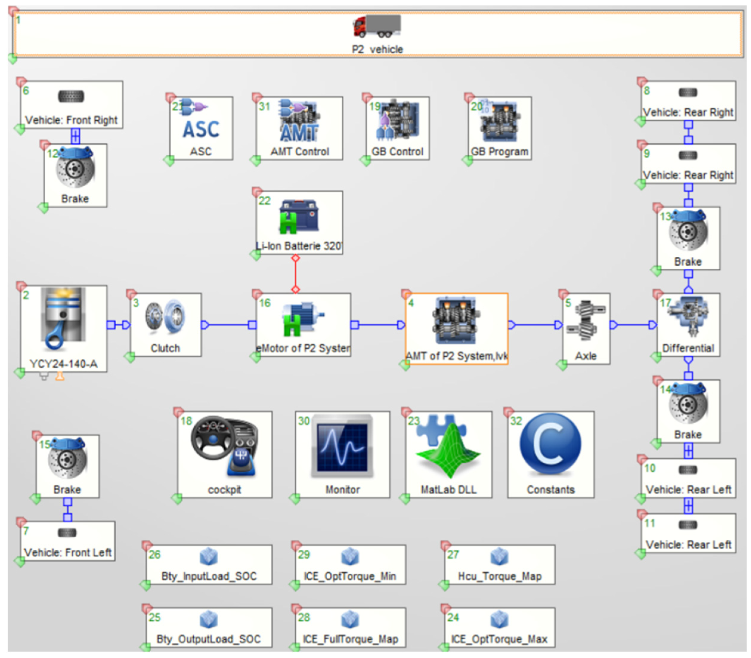
In this study, the P2 hybrid commercial vehicle was selected as the model, and its topology is shown in Figure 1. The electric motor of the P2 hybrid vehicle is located between the combustion engine and the transmission, and the torque coupling between the electric motor and the combustion engine is controlled by the clutch, so that different vehicle control and energy management strategies can be set, to achieve different driving modes and improve the overall vehicle dynamics and fuel economy [20]. With the rapid development of new energy vehicles, the P2 structure has been widely adopted by major manufacturers due to its low cost [21]. Table 1 shows the vehicle parameters of the hybrid vehicle.
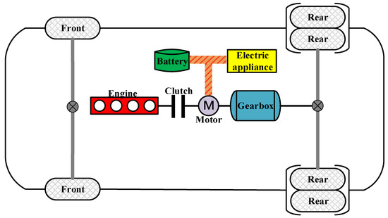
Figure 1.
Structure of the HEV.

Table 1.
Vehicle parameters.
2.1. Vehicle Model
When a car travels, it must overcome rolling resistance, air resistance, gradient resistance, and acceleration resistance; thus, the following equation for the car’s movement can be formed:
where is the driving force, and it can be expressed in terms of:
where is the combustion engine torque; is the transmission ratio; is the main transmission ratio; is the transmission efficiency; is the tyre radius; is gravity; is the tyre rolling resistance coefficient; is the slope angle; is the air resistance coefficient; is the upwind area; is the car velocity; is the mass conversion coefficient; and is the total mass of the car.
2.2. Combustion Engine Parameter Matching
The performance of the car cannot be sacrificed when improving its economy. The performance index for a car is assessed using the maximum speed , acceleration time and maximum gradient climb [22]. Regarding the pure combustion engine drive, when the car is at maximum velocity under the demand power and the maximum gradient-climbing demand power needed to produce the total combustion engine power , both need to satisfy the following formula:
- The total power is determined from the maximum velocity.
- 2.
- The total power is calculated based on the maximum gradient climbed.
In summary, the main combustion engine parameters are obtained, as shown in Table 2:
Table 2.
Combustion engine parameters.
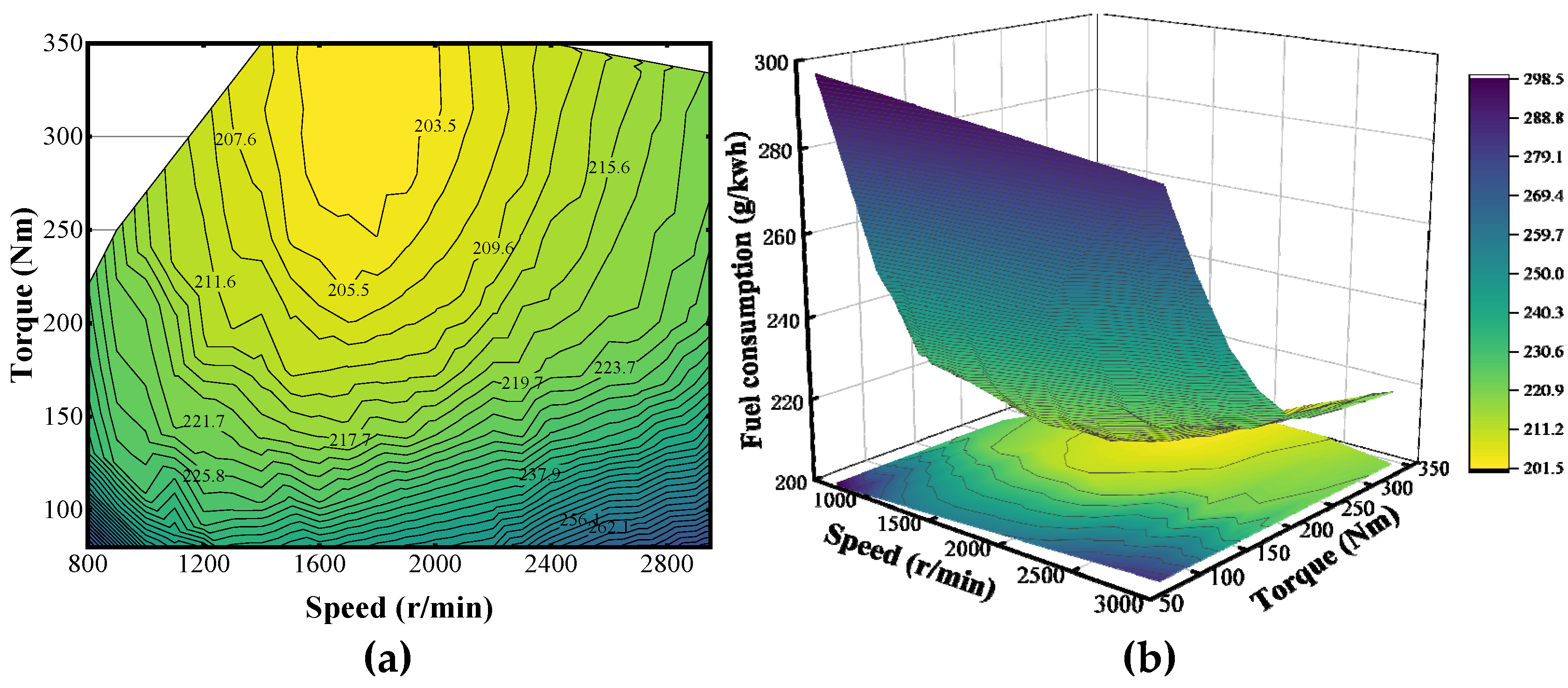
Two- and three-dimensional contour maps of the combustion engine are shown in Figure 2.

Figure 2.
(a) Two-dimensional contour map of combustion engine; (b) three-dimensional contour map of combustion engine.
2.3. Electric Motor Parameter Matching
When the electric motor is driven alone, it is necessary to simultaneously satisfy the demand power at maximum velocity in EV mode, the demand power at the maximum gradient climb, and the demand power at maximum acceleration, where and should be kept equal to the electric motor parameters.
Neglecting the gradient resistance, the electric motor power demand is calculated from the maximum acceleration as:
where is the final velocity of acceleration, km/h; is the total time of acceleration, s; and is the fitting coefficient, taken as 0.5.
The maximum electric motor speed is calculated using the following formula:
The electric motor rated speed is calculated using the formula:
where is the maximum velocity; is the main deceleration ratio; is the tyre radius; and is the expanded constant power zone coefficient, which takes the value of 2.
The torque of the electric motor can be obtained from Equation (9).
In summary, the main electric motor parameters are obtained, as shown in Table 3.
Table 3.
Electric motor parameters.
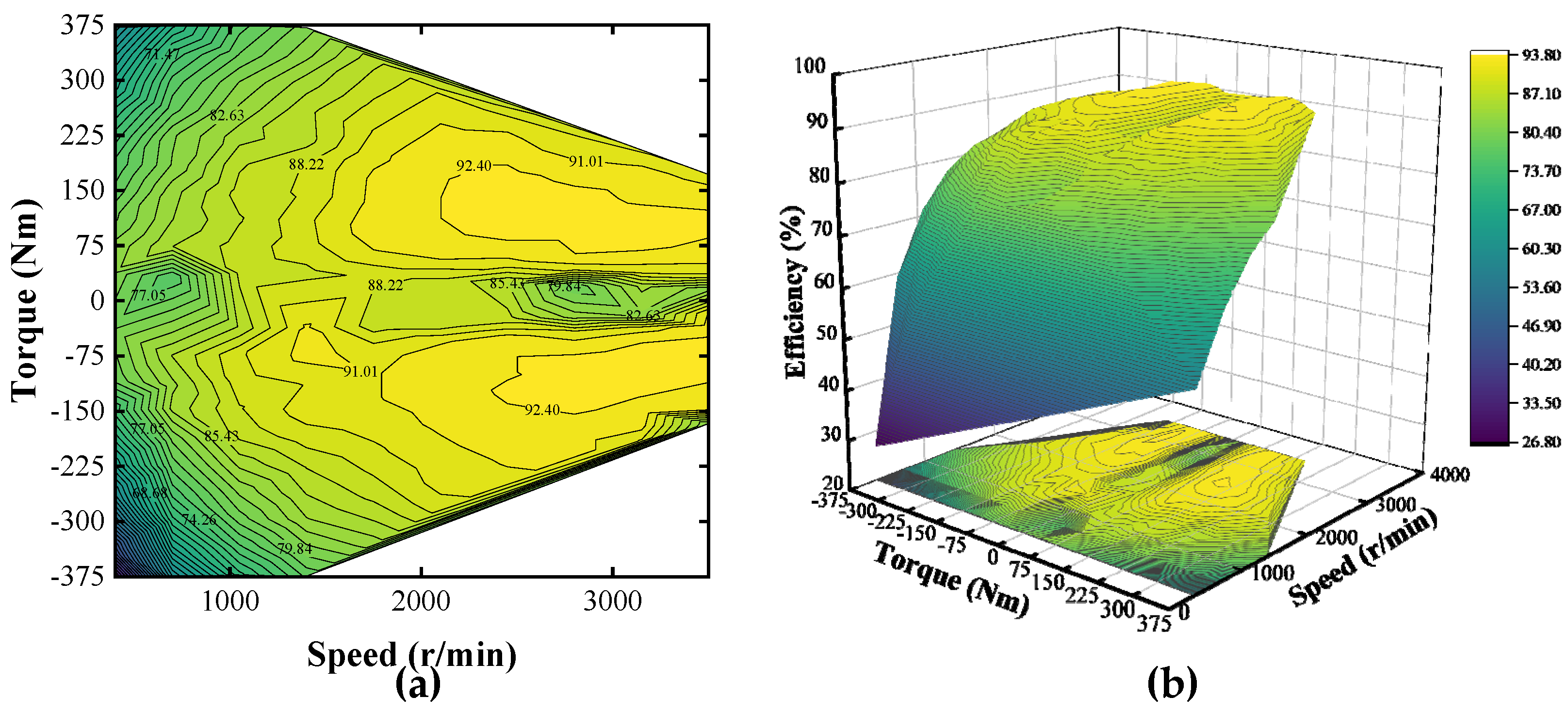
Two- and three-dimensional efficiency maps of the electric motor are shown in Figure 3.

Figure 3.
(a) Two-dimensional efficiency map of electric motor; (b) three-dimensional contour map of electric motor.
2.4. Power Battery Models
The power battery is mainly used to provide power to the electric motor; taking into account the role of energy recovery, the battery pack in this study consisted of 550 single lithium batteries. The relationship between the rate of change and the current is as follows:
The capacity of the power battery pack can be calculated based on the nationally specified range, the target constant velocity, and the power requirement of the electric motor. The capacity requirement for the power battery pack for the target range is:
where is the uniform velocity; is the target driving range; is the working efficiency of the electric motor; is the voltage of the power battery pack; and is the power required by the electric motor.
2.5. Vehicle Model Construction
AVL-Cruise v.2019 is a piece of software developed by AVL for the power components of the whole vehicle; it can be used to study the fuel consumption and dynamics of different vehicles under different working conditions. The way the software divides the whole vehicle into several small modules makes it easy for the user to build different vehicle models according to their own ideas, and its complete solver can quickly output accurate results; therefore, AVL-Cruise v.2019 software was used in this study, and whole-vehicle modelling was carried out based on the topology of the P2 hybrid vehicle as described in the previous section. The specific steps are as follows:
Step 1: According to the structure of the P2 hybrid vehicle, build the mechanical connection model between the vehicle, wheels, combustion engine, electric motor, clutch, transmission, brake, power battery, main reduction gear, and differential, etc., in Cruise.
Step 2: Enter the basic parameters of the whole vehicle and the parameters of the selected components.
Step 3: Set the mechanical and electrical connections, outputs, and output signals between the components.
Figure 4 shows the Cruise vehicle model created in this study.
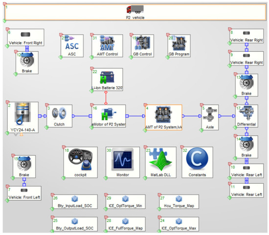
Figure 4.
Cruise complete vehicle model.
3. Working Condition Identification Model Construction
3.1. Data Pre-Processing
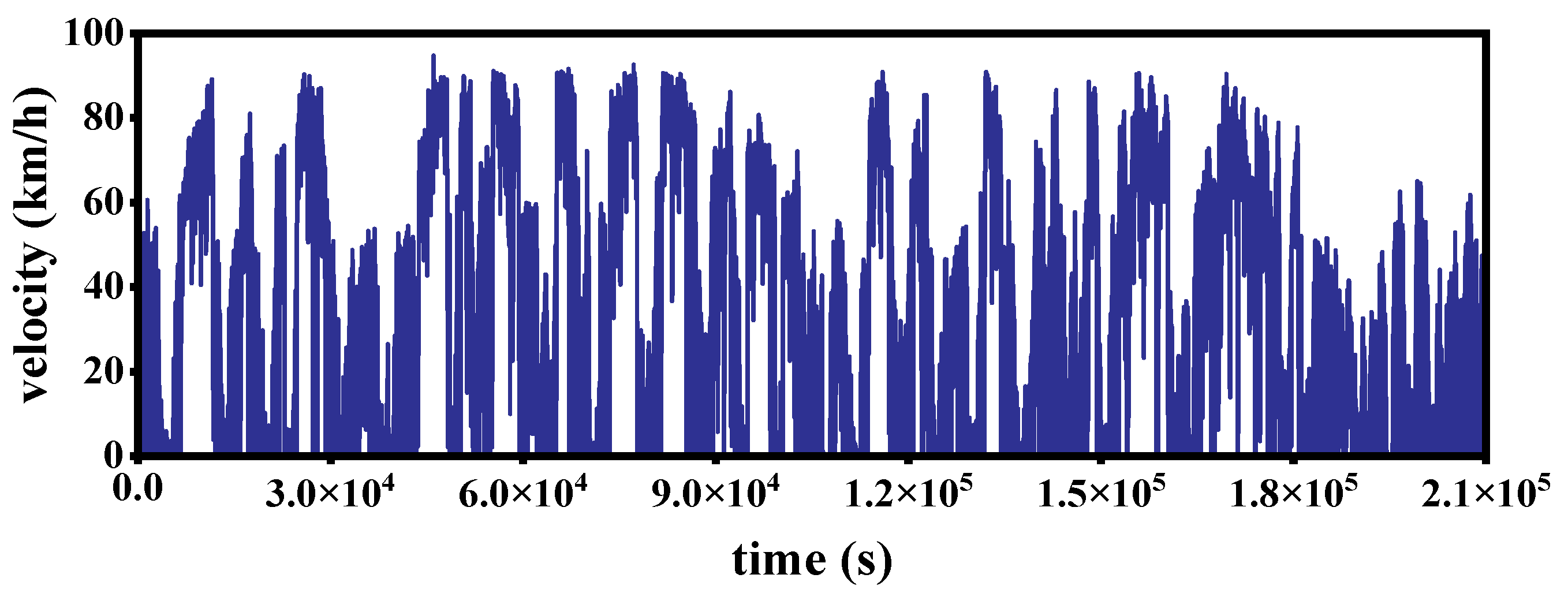
In this study, the data collected came from the driver’s random autonomous driving, which is random and more responsive to the road driving characteristics in the region and the driving needs of ordinary drivers. Some of the time–velocity information is shown in Figure 5.
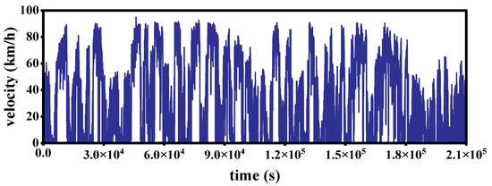
Figure 5.
Partial velocity clip.
It is particularly important to pre-process the data to ensure that they are accurate and reliable. In this study, the data were pre-processed as follows:
When the data distortion was greater than 5 s, the distorted work segment was excluded, and for the part less than or equal to 5 s, the mean value was used to make up the difference. The formula for this is as follows:
where is the velocity at the point of distortion; is the velocity one second before the distortion; and is the velocity two seconds before the distortion.
The complete dataset after the complementary difference adjustment was subjected to wavelet filtering. According to the multi-scale transformation of wavelet filtering, the signal noise was classified into low- and high-frequency signals, and the noise was usually a high-frequency signal. The one-dimensional noise signal can be expressed as:
where is the original signal; is the real signal; is the noise standard deviation; and is the noise.
In the wavelet denoising process, the original signal was first decomposed, and then each layer was processed using thresholding; finally, the signal was reconstructed after each layer had been processed. The continuous wavelet transform for any function is:
where is the scaling factor; is the translation factor that changes the displacement of the continuous wavelet; is the discrete wavelet transform of ; and the discretisation method is , where is the set of integers. In this study, soft-threshold signal processing was chosen, and its expression is as follows:
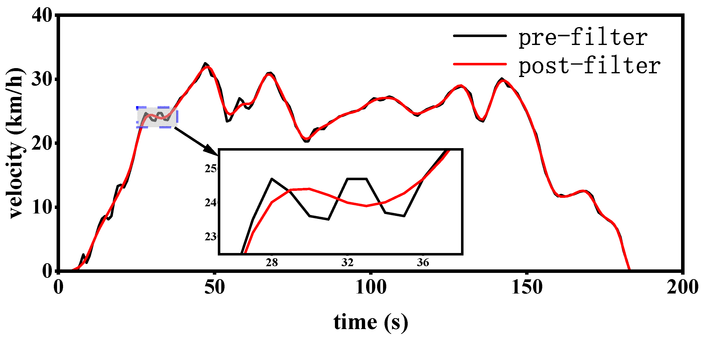
where is the wavelet coefficient and is the threshold. If the absolute value of the wavelet coefficient was equal to the given threshold, it was subtracted from the threshold, and if it was less than the given threshold, it was set to 0. Due to the large size of the original data, filtering was implemented. Figure 6 shows some of the velocity segments after filtering.
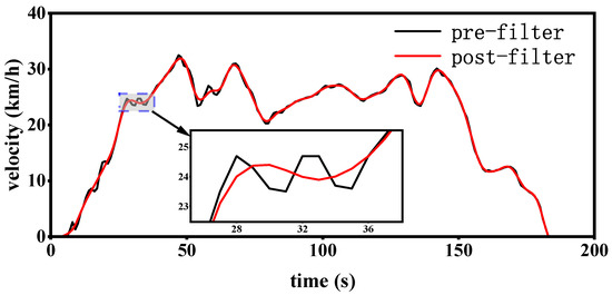
Figure 6.
Some clips before and after filtering.
3.2. Classification of Working Conditions
In this study, the working condition classification was based on a number of kinematic segments; each kinematic segment had different characteristics, so the pre-processed driving condition time series were divided into kinematic segment libraries, the data from which were the basis for the working condition classification. The processed vehicle velocity was divided into kinematic segments, and the pre-screening process was as follows:
Step 1: Due to the large timespan of the collected data, there were a large number of idle segments on the road; idle segments of >200 s were reduced to 200 s to meet the requirements of kinematic segments.
Step 2: This paper focuses on the study of commercial vehicles; according to the actual situation, the acceleration and deceleration speed should be less than 5 m/s2, so it was necessary to omit kinematic segments with acceleration and deceleration speeds greater than 5 m/s2.
The kinematic segment feature parameters can be used to describe themselves; however, due to certain correlations between the feature parameters, too many feature parameters would make the information redundant. Therefore, this study selected parameters based on relevant research [23,24,25]. The following were chosen as the characteristic parameters of kinematic segments: acceleration segment average acceleration (); deceleration segment average deceleration (); maximum deceleration (); maximum acceleration (); deceleration ratio (); acceleration ratio (); stopping ratio (); motion ratio (); average running velocity (); maximum velocity (); and average velocity (). Table 4 shows the characteristic data of the kinematic segments.
Table 4.
Characteristic values of kinematic fragment library.
The high dimensionality of the original feature parameter data, and the presence of a large data overlap, increase the computational complexity of K-means cluster analysis [26]. Principal component analysis (PCA) replaces the original data feature parameters with fewer principal components by mapping the high-latitude feature parameters to the low-latitude ones; after the dimensionality reduction, each feature of the data is independent of the others, and if the data are affected by noise, discarding some of the data can help to reduce noise. Therefore, the data’s dimensionality was reduced using PCA. The principal components of the kinematic fragment library and their contribution values were obtained according to the PCA step in the literature [27], as shown in Table 5.
Table 5.
Principal component eigenvalues and contributions.
As shown in Table 5, the cumulative contribution rate of the first four principal components reached 87.077%, which is sufficient for characterising all the feature information of the driving condition data in this paper, and the first four principal components were selected as the clustering features.
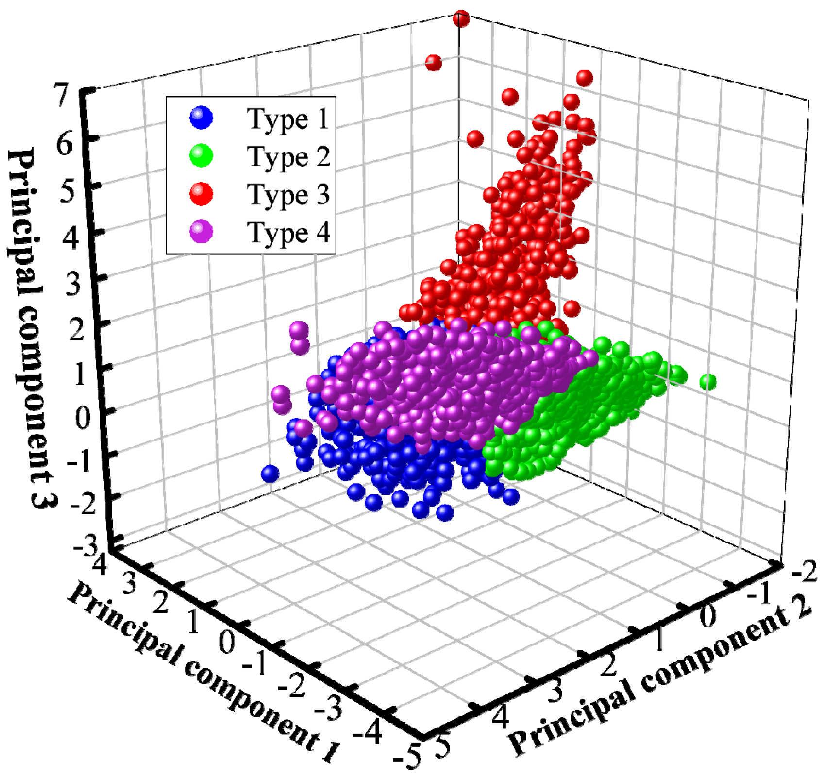
According to the characteristics of the driving condition kinematic segments, the K-means algorithm was used to cluster the segments; the K-means algorithm converges faster and can overcome the shortcomings of spectral clustering, making the classification results more accurate and reasonable. According to the K-means clustering steps outlined in the literature [28], this study finally clustered the original data into four categories. Figure 7 presents a clustering effect diagram.

Figure 7.
Clustering effect.
In Figure 7, Type 1, Type 2, Type 3 and Type 4 are the scatter plots of four categories under the dimensions of Principal Component 1, Principal Component 2 and Principal Component 3, which demonstrate that there are clear boundaries between the categories, that the distribution patterns are clearly unique, and that there are fewer samples in each category that deviate significantly from the centre of the clusters, suggesting that the clustering works well.
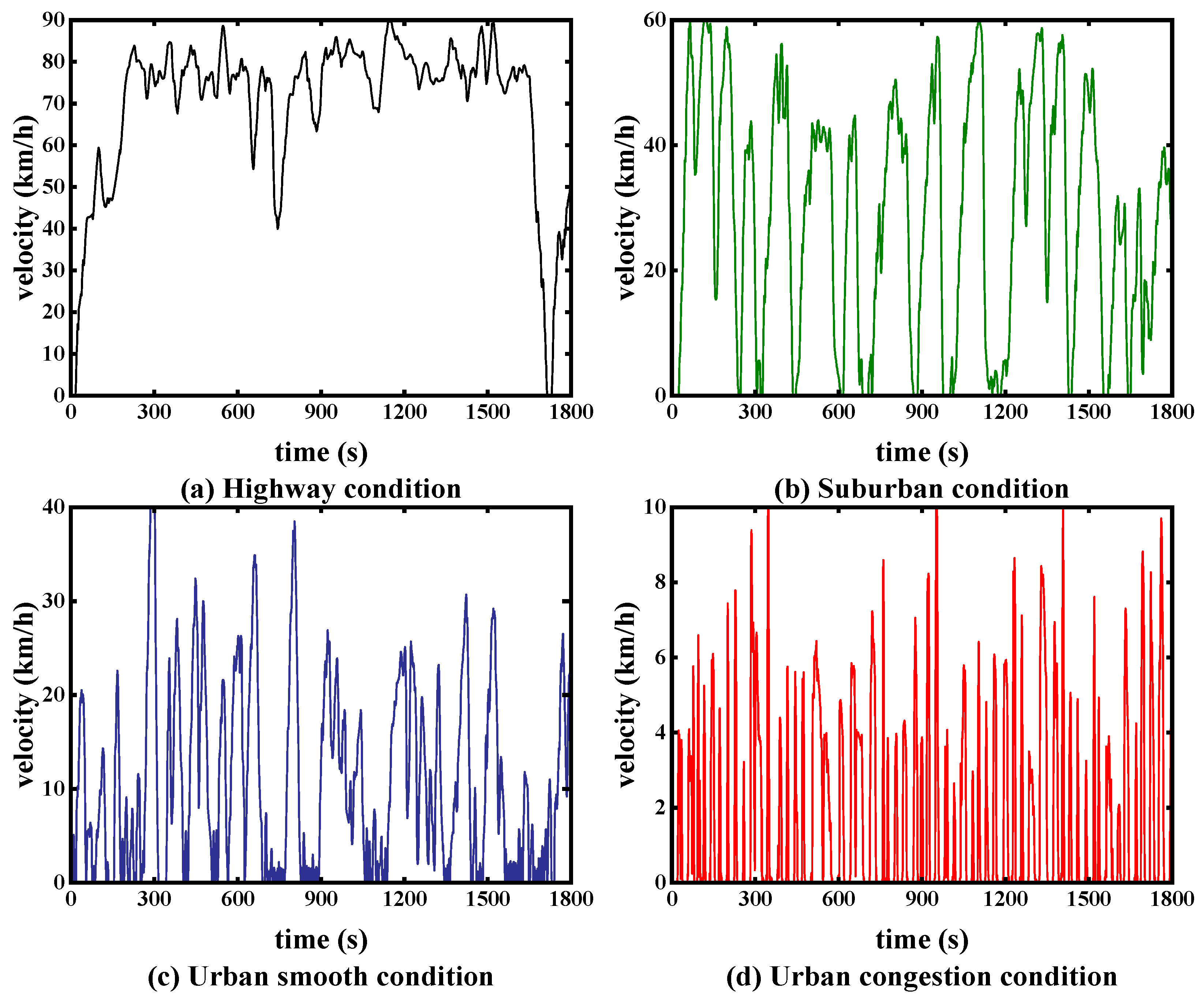
Figure 8 shows the results of the category of working conditions. As can be seen in Figure 8, the variability of the characteristics of the four categories is distinct. Figure 8a shows the highest velocity, maintained close to 90 km/h, with a short idle time, low number of times, and high velocity maintained for a long time, reflecting highway conditions. Figure 8b shows the maintenance of the velocity close to 60 km/h; compared to the working condition (a), the number of idle times is increased, the idle time is increased, and the duration of high velocity is moderate, which corresponds to the working conditions of suburban environments. Figure 8c shows that the velocity is kept close to 30 km/h, the number of start–stops is higher, the idle time is longer, and the velocity fluctuation is greater, corresponding to the working conditions of a smooth urban environment. Figure 8d shows the lowest velocity, below 10 km/h; the start–stops are frequent, the idle ratio is large, and the high velocity is maintained for a short period of time, which is in line with the low-velocity working conditions of urban congestion.
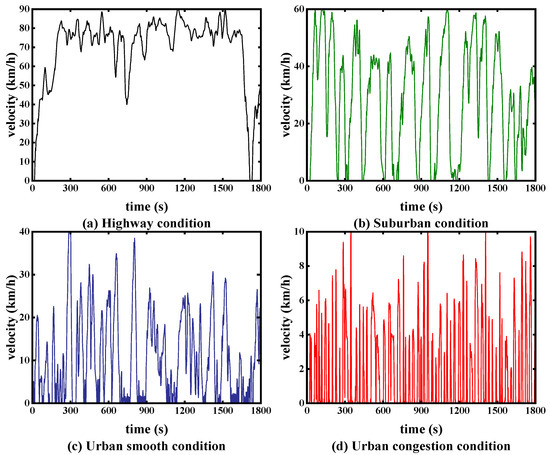
Figure 8.
Classification results for typical working conditions.
3.3. COA-BPNN Working Condition Identification Construction
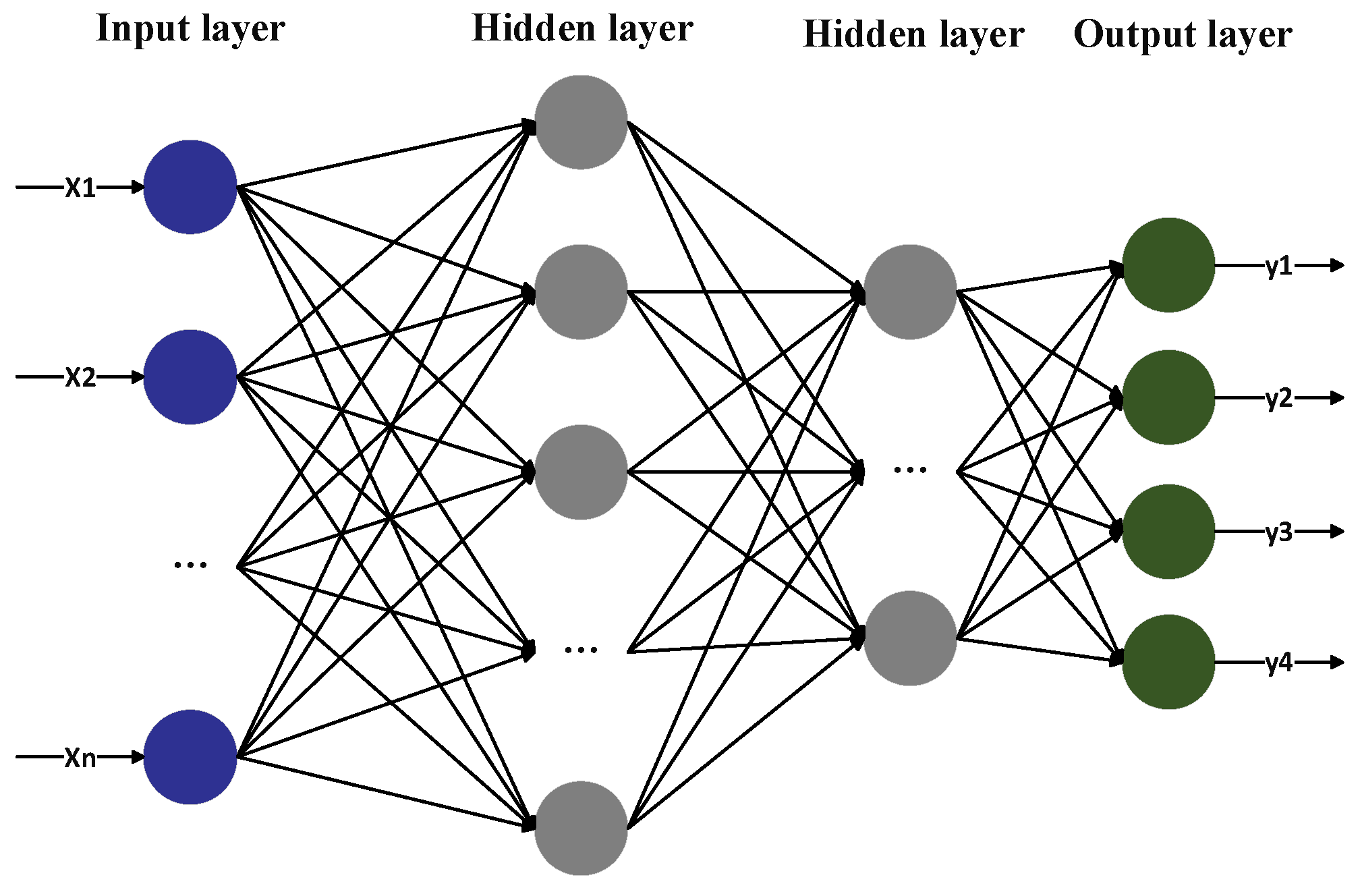
The backpropagation neural network (BPNN) is a multilayer feedforward neural network trained using error backpropagation. Due to the learnability of its weights and thresholds, the BPNN has a strong nonlinear fitting ability and works better for category recognition [29]. The BPNN consists of an input layer, hidden layer, and output layer, and its structure is shown in Figure 9.

Figure 9.
BPNN structure.
Where are input neurons and are output neurons. The output thresholds of the hidden layer and the output layer are and , respectively, where the input layer is the characteristic parameter of the driving conditions and the output layer is the category of the working conditions. The weights of the neuron connections between the input layer and the implicit layer, and between the implicit layer and the output layer, are , respectively. , and directly affect the recognition accuracy of the BPNN and reduce the accuracy of work recognition; thus, this study, with the help of the COA intelligent optimisation algorithm proposed by Mohammad et al. [30], took advantage of the higher convergence speed of the COA algorithm and the ability of global optimisation to search for , and and obtain the optimal solution to be applied to the BPNN. The specific steps of the COA-BPNN algorithm are as follows:
Step 1: Population initialisation. Translate , and to each Coati position. Determine the population size and the maximum number of iterations .
Step 2: Find the best individual position in the population.
Step 3: Update the position. If the new position improves the value of the objective function, the new position is acceptable; otherwise, the raccoon stays put. Use the average of the squared error between the actual output and the desired output as the fitness function.
Step 4: Coati avoidance strategy.
Step 5: Greedy selection. If the computed position improves the value of the objective function, it is acceptable; otherwise, keep it as it is.
3.4. COA-BPNN Working Condition Identifier Verification
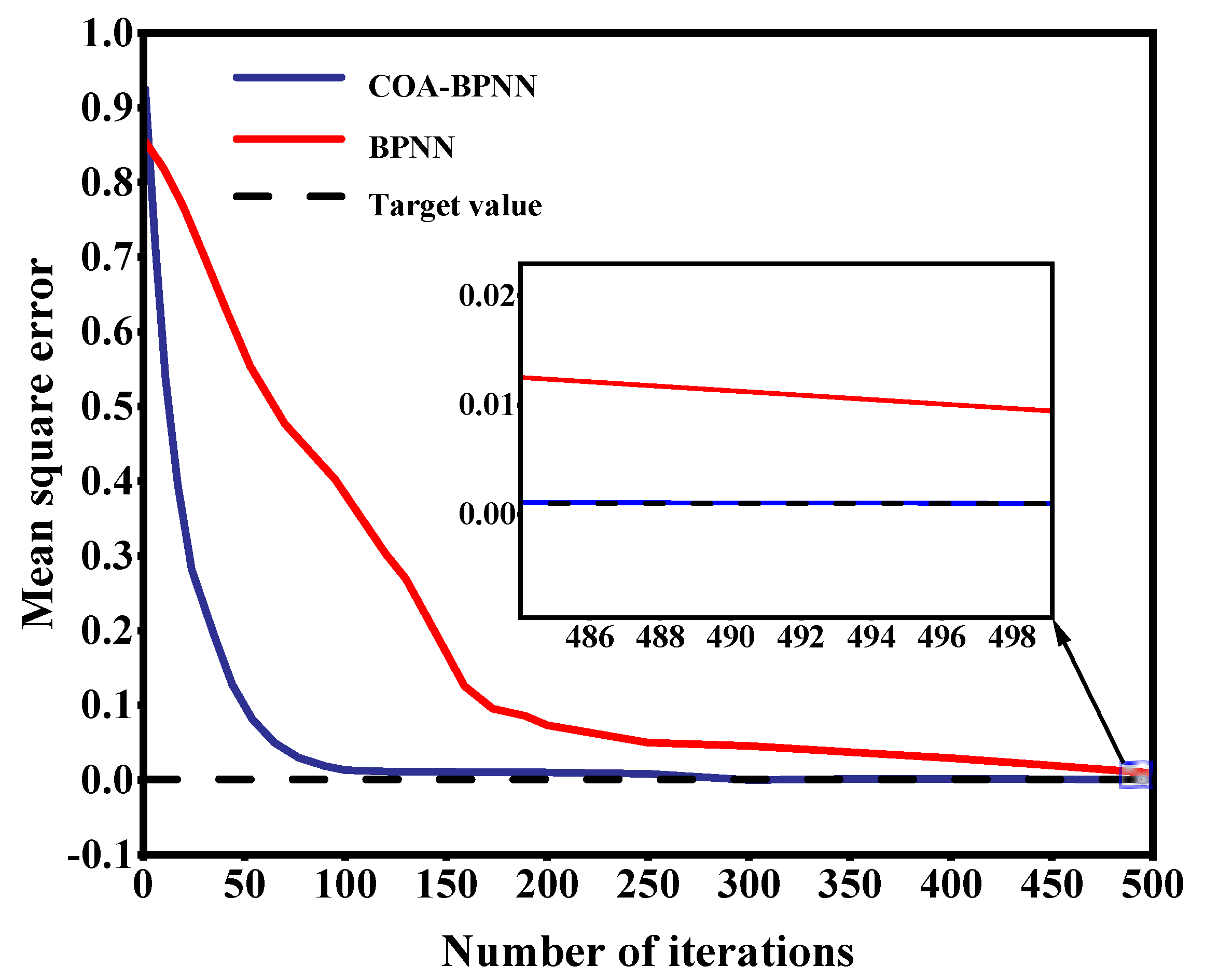
Online working condition identification was used to retrieve the characteristics of the historical time window during driving and identify the category of the current time window . As explored in Section 3.2, the data of the four working condition category combinations were divided according to the 10 s historical time window, and the total number of samples was set to 1800; 70% was selected as the training set, 20% was used as the test set, and 10% was used as the validation set. The number of iterations was set to 500, and the target accuracy of iteration was 0.001. Each window feature parameter was calculated as the training data. The number of nodes in the input layer of the BPNN was 11, the number of nodes in the hidden layer was 15, and the number of nodes in the output layer was 4.
Figure 10 shows a comparison of the iteration process between COA-BPNN and BPNN. As can be seen in the figure, after 100 iterations, the mean square error of the COA-BPNN algorithm was stable, and the convergence speed was significantly higher than that of the BPNN. When the iteration was carried out 500 times, the final mean square error of the COA-BPNN was 0.001 and that of the BPNN was 0.009, which shows that the recognition accuracy of the COA-BPNN was significantly superior to that of the BPNN, which reached 98.9%.

Figure 10.
Comparison of COA-BPNN and BPNN iterations.
4. Construction of Regenerative Brake Strategy Based on Condition Identification
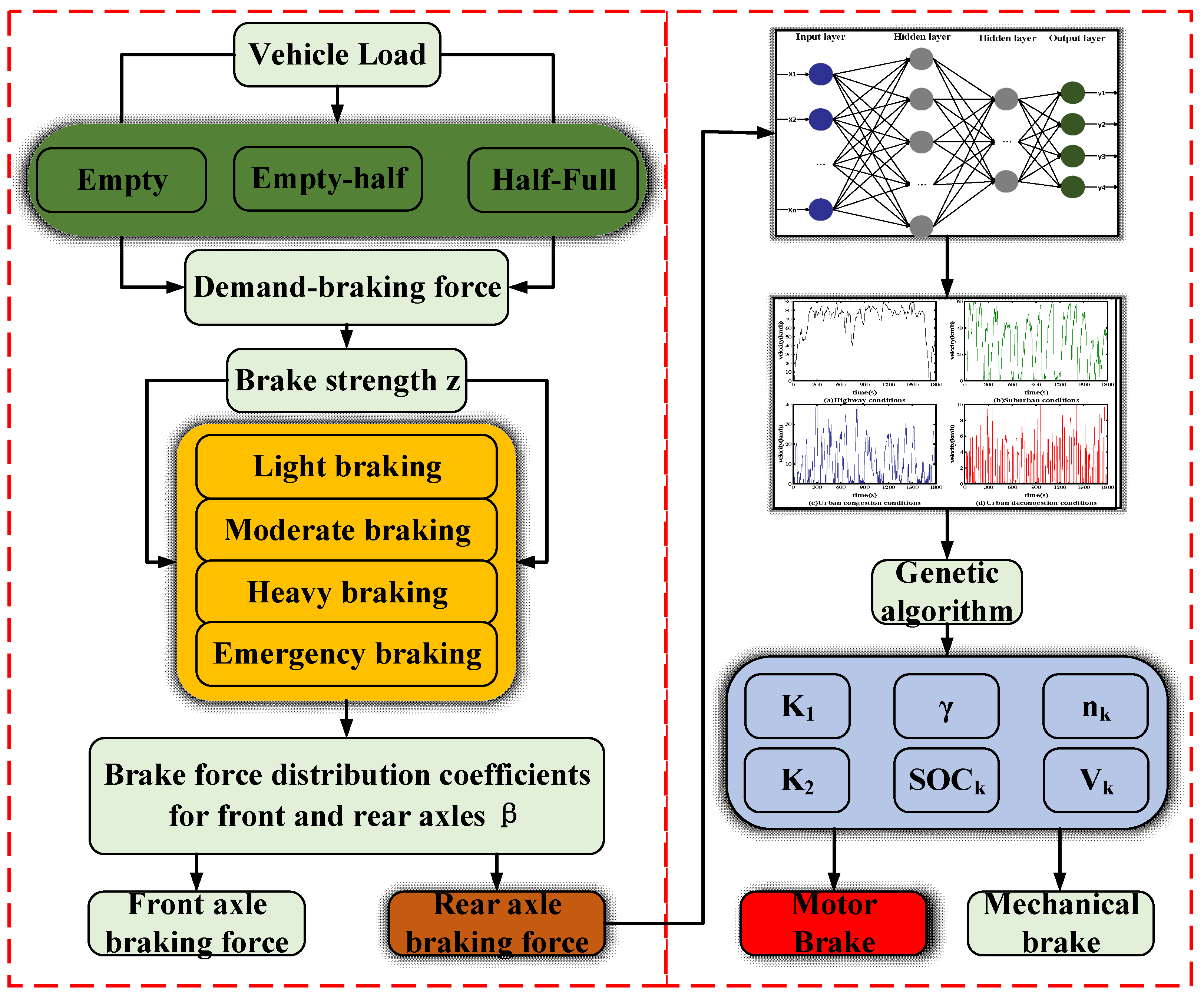
This section describes how a distribution strategy was designed to develop the front and rear axle braking force distribution coefficients as a variable ratio value, based on the no-load, half-load and full-load braking force. Then, based on the six key control parameters affecting the electric motor braking energy recovery efficiency, each category of working conditions derived from the clustering in Section 3 was individually treated as a working condition velocity, and a genetic algorithm was used to determine the optimal control parameters for the three kinds of loads under each category of working conditions; then, through the COA-BPNN online working condition recogniser, the algorithm identified the current category of working conditions and retrieved the corresponding optimal control parameters in the offline parameter library, and the electric motor demand braking force and mechanical braking force were calculated. Figure 11 shows the framework of the condition recognition-based regenerative braking strategy.

Figure 11.
Structure of regenerative braking strategy based on condition recognition.
4.1. Front and Rear Axle Brake Force Distribution Strategy
4.1.1. Front and Rear Axle Brake Force Distribution Curve Analysis
- Ideal brake force distribution curve
In the braking process, when the braking force can meet the vehicle braking conditions, the front and rear wheels exhibit the following three states: first, the front wheels take the lead in holding and slipping; second, the rear wheels take the lead in holding and slipping; third, the front and rear wheels are simultaneously responsible for holding and slipping. These are the most ideal conditions, as they can avoid rear axle side slip, ensuring the best utilisation rate for adhesion under these conditions, thereby meeting the requirements of vehicle braking safety and stability. At this point, both the front and rear wheels can be in an ideal state of holding dead simultaneously. This occurs when the front and rear axle braking force distribution curve forms what is referred to as an curve. The formula for the ideal braking relationship function between the front and rear axle braking forces is as follows:
where is the front axle brake force; is the rear axle brake force; is the wheelbase of the vehicle; is the gravitational force of the vehicle; is the height of the centre of mass of the vehicle; and is the distance from the rear axle to the centre of mass of the vehicle.
- 2.
- ECE regulation requirements
For lorries with a gross mass of more than 3.5 tonnes, the UNECE braking regulation ECER13 sets out requirements for the distribution of braking force between the front and rear axles of such vehicles. The distribution of braking force between the front and rear axles is expressed by the braking force distribution coefficient , i.e., the ratio of the braking force of the front axle and the total braking force required by the vehicle. According to an analysis of the regulation, the front and rear axle brake force distribution coefficient and the braking intensity are defined as follows:
4.1.2. Front and Rear Axle Brake Force Distribution Strategy
According to the level of braking intensity, braking is divided into four modes: light, medium, heavy, and emergency braking. As the rear wheel first locking in the braking process represents an unstable condition, an empty-, half-, and full-load/front- and rear-axle braking force distribution strategy was developed, based on the comprehensive consideration of the f-group line (the front wheel first locking and the rear wheel not being wrapped), ECE braking regulations, and the ideal braking force distribution curve of different loads. Brake force distribution curves for the front and rear axles are shown in Figure 12.
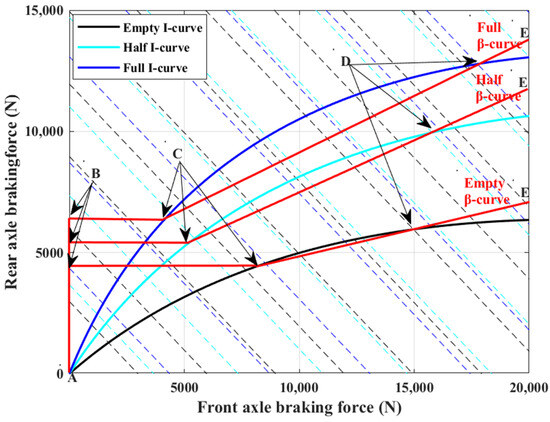
Figure 12.
Brake force distribution curves for front and rear axles.
As shown in Figure 12, the brake force distribution rules are as follows:
- (1)
- Light braking mode: When the braking intensity is between 0 and 0.15 (), regardless of the current vehicle load, all of the braking force is distributed to the rear axle according to the AB curve. The maximum braking force is provided by the electric motor, and the mechanical brake plays a complementary role.
- (2)
- Medium braking mode: The vehicle distributes the braking force according to the BC curve, the braking force of the rear axle remains unchanged, and the braking force of the front axle increases linearly with the increase in braking intensity, until the no-load threshold , half-load threshold , and full-load threshold are reached.
- (3)
- Hard braking mode: The vehicle distributes the brake force along the CD curve, and the brake force distribution curve is always below the ideal brake force distribution coefficient curve and close to the I curve, until it coincides again with the ideal brake force distribution coefficient curve, at which point .
- (4)
- Emergency braking mode: If , no regenerative braking is performed under any load condition, and the braking force is fully distributed to the mechanical brakes of the front and rear axles, according to the DE curve.
4.2. Optimisation of Regenerative Braking Parameters Based on GA
The efficiency of regenerative braking energy recovery is mainly affected by the vehicle velocity, battery charge state, battery charging power, electric motor characteristics, and the ratio of brake force distribution between mechanical and electric motor; the braking torque requirement of the electric motor can be calculated using the following equation:
where is the vehicle demand brake torque; is the electric motor brake demand torque; is the velocity correction factor; is the correction coefficient; is the transmission efficiency; is the electric motor brake demand torque gain coefficient; and is the mechanical and electric motor brake force distribution coefficient, i.e., the ratio of the electric motor brake torque to the total brake torque of the rear axle.
When , the battery limits the maximum charge power to limit the power generated by the electric motor, thus extending the life of the battery.
where is the generating power of the electric motor; is the maximum charging power of the battery; and is the maximum charging power gain coefficient of the battery.
The electric motor speed affects the efficiency of the electric motor’s power generation, and the regenerative braking minimum electric motor speed keeps the electric motor in a more efficient working range.
where is the power at minimum speed and is the minimum speed of regenerative braking, in rpm.
In this study, the velocity correction factor was set within the range [0.8, 1.2]; the battery SOC correction factor was set within the range [0.8, 1.2]; the electric motor braking demand torque gain coefficient was set within the range [1, 4]; the maximum battery charging power amplification coefficient was set within the range [0.5, 1]; the minimum speed of the electric motor for regenerative braking was set within the range [400, 800]; and the mechanical and electric motor braking force distribution coefficients were optimised in the range [0, 1] to obtain the best regenerative braking energy recovery efficiency.
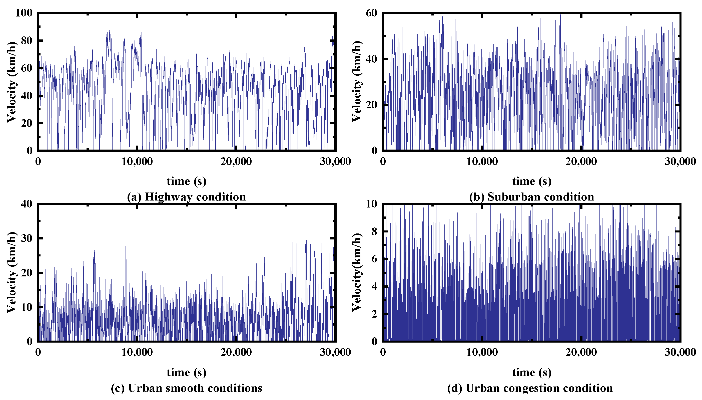
Four driving conditions were defined and obtained, as described in Section 3; Figure 13 shows some of the time–velocity curves synthesised for the four conditions, where (a), (b), (c), and (d) were synthesised using only kinematic segments of the highway, suburban, urban smooth, and urban congestion working conditions, respectively, and parameter optimisation was performed under each of the four conditions.
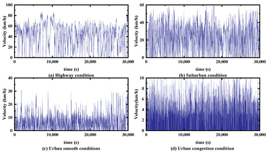
Figure 13.
Time–velocity curves for four conditions.
The genetic algorithm (GA) is an adaptive global search method for finding optimal solutions through the simulation of the evolutionary process, which defines the search space of optimal solutions as an evolutionary process and solves them with a set of stochastic rules. GAs do not have the restriction of the hard rules found in traditional algorithms, giving them superior parallel solving abilities and global optimality search abilities, and they can also effectively solve multi-objective optimisation problems; therefore, a GA was chosen for offline parameter determination in this study. The steps of the GA used in this study for parameter optimisation were as follows:
Step 1: The target parameters and their constraints were determined, and the six control parameters were formed into an individual component of the genetic algorithm.
Step 2: The target working conditions and the target load state were determined. The four synthetic working conditions clustered above were used to run the strategy separately, to derive the optimal control parameters under different working conditions.
Step 3: Coding and population initialisation. The binary coding method was used to encode the six control parameters into individuals; the random method was used to initialise the population.
Step 4: Setting and calculating the fitness function. Considering the brake energy recovery efficiency and brake safety, the sum of the minimum brake energy loss and brake safety was selected as the objective function, as shown in Equation (25).
where decreases as the braking intensity becomes larger, and vice versa for . Equation (26) is the weighting factor rule.
Step 5: According to the degree of adaptation of the individual determining the probability of the individual to be selected, the better the adaptation of the individual, the greater is the probability of being selected.
Step 6: If the value of the objective function satisfies the condition or reaches the maximum number of iterations, then stop the iteration and output the optimal value; if it does not satisfy the condition, then return to Step 4.
Table 6 shows the values of the optimum control parameters for different loads, obtained according to the above steps.
Table 6.
The optimal control parameters of different loads under four working conditions.
4.3. Regenerative Braking Strategy Modelling Based on Condition Identification
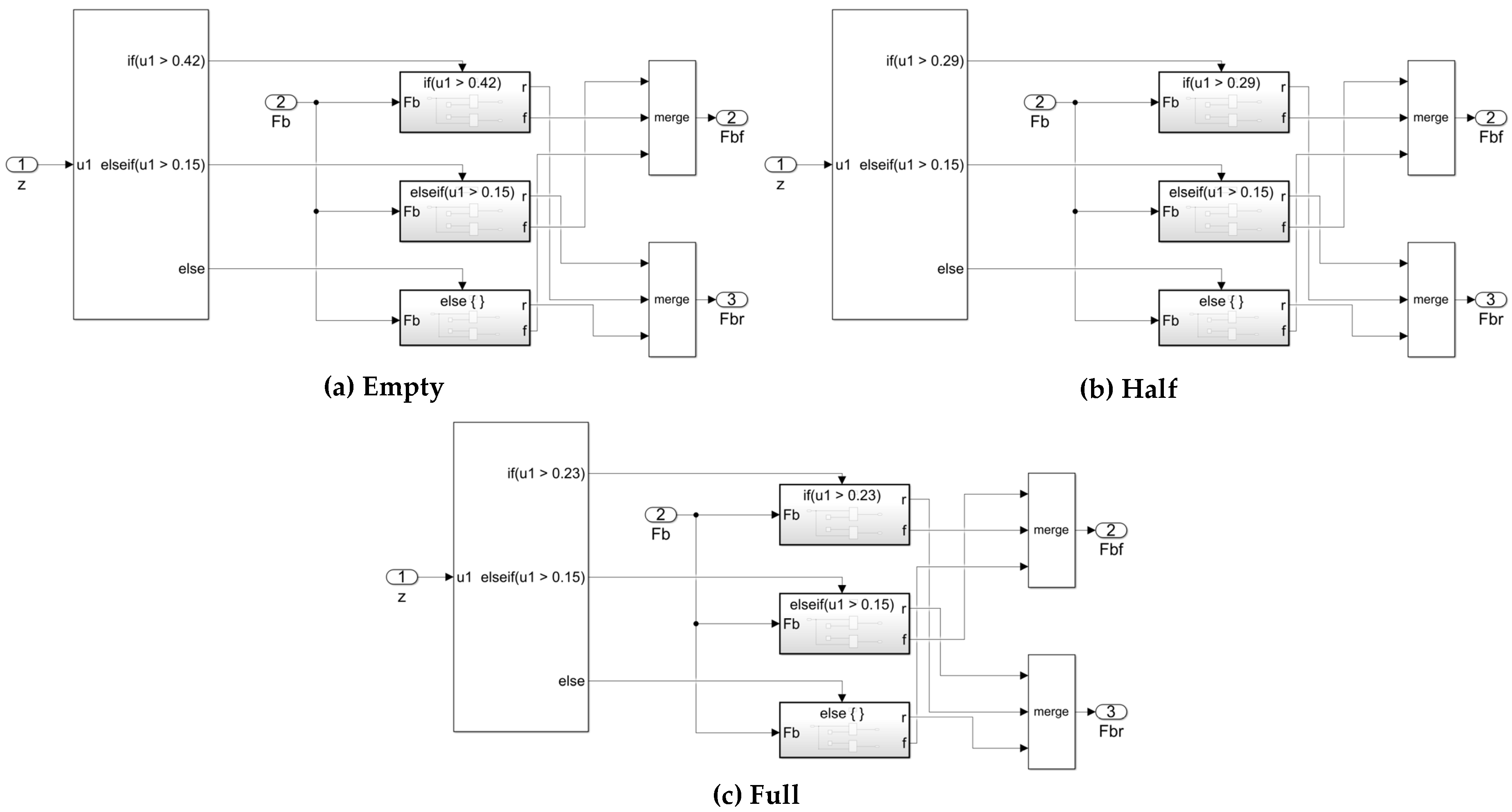
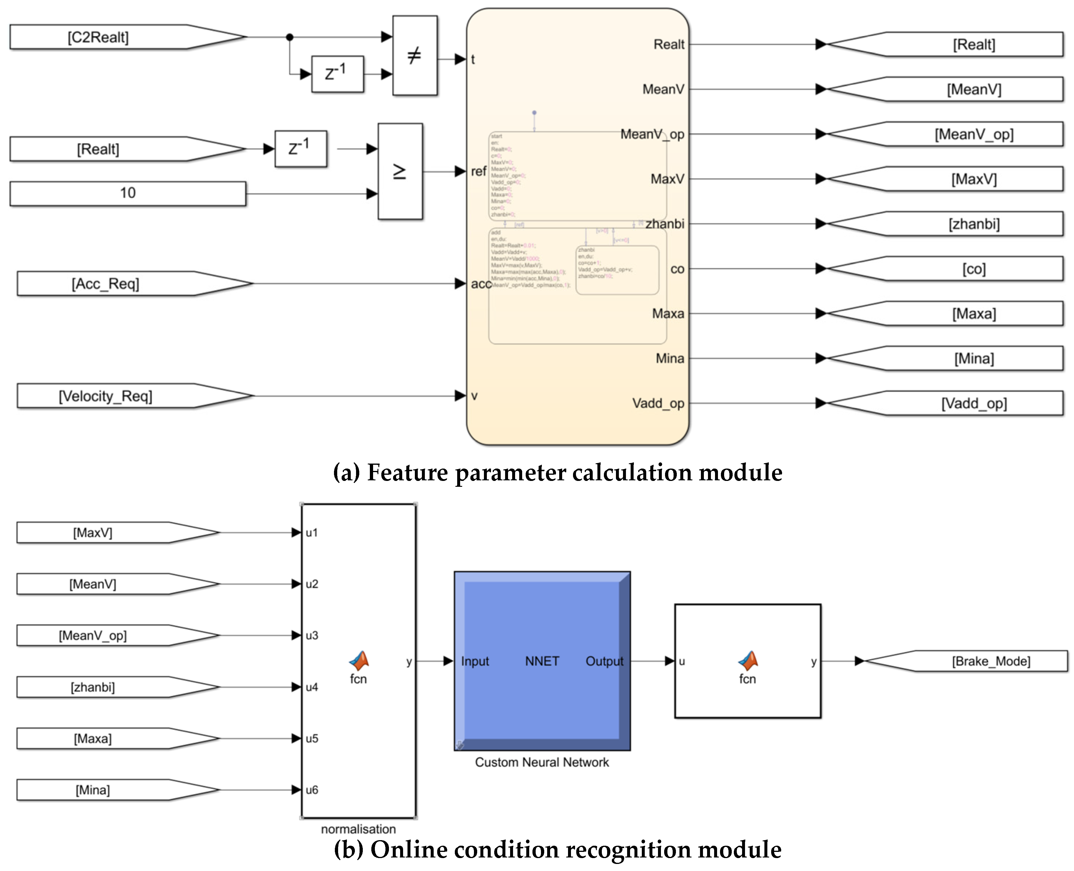
Simulink is a visual simulation tool in Matlab that is widely used in modelling and simulation applications for linear systems, nonlinear systems, digital control, and digital signal processing, and it can convert the constructed control model into a DLL file to perform data transfer and a joint simulation with AVL-Cruise software to improve research efficiency. Thus, based on the regenerative braking strategy designed in the previous chapters, in this study, the regenerative braking strategy model based on condition identification was built in Simulink, as shown in Figure 14 and Figure 15.
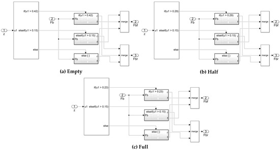
Figure 14.
(a) Brake force distribution on front and rear axles in empty-load state; (b) brake force distribution on front and rear axles in half-load state; (c) brake force distribution on front and rear axles in full-load state.
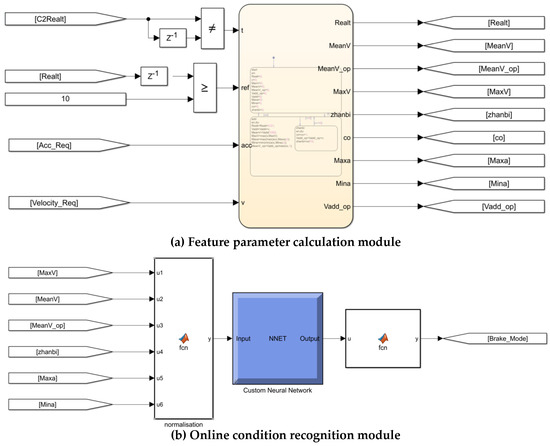
Figure 15.
(a) Feature parameter calculation module; (b) online condition recognition module.
5. Simulation Analysis
The most commonly used verification method in the simulation process of energy management strategy construction is Matlab/Simulink 2022(a) and AVL-Cruise v.2019 joint simulation. To ensure the rigour of the simulation, the C-WTVC cycle, and a sampling synthesis of the cycle based on the clustering results of the previous paper, were selected. The joint simulation analysis was conducted using the Matlab DLL interface method to verify the design of this paper’s control strategy’s effectiveness. With reference to the duration of the international standard conditions, the duration of the synthetic cycle in this study was set to 1800 s, in which the duration of each type of conditions was determined according to the following formula:
where is the duration of the i category of the synthetic conditions; is the time occupied by the ith category of all kinematic segments; is the duration of all kinematic segments; and is the target duration of the synthetic conditions.
To ensure that the research was rigorous, a fixed-ratio strategy where and , and a fuzzy control strategy with the vehicle velocity, , and brake pedal opening as inputs, and the electromechanical brake force distribution as the output, were selected for comparison in the simulation process for the simulation analysis.
The braking energy recovery rate, i.e., the ratio of energy recovered to the energy consumed during braking, was used as an evaluation index for the simulation, as shown in Equation (28).
where is the brake consumption energy recovery rate; is the recovered energy (kJ); and is the consumed energy (kJ).
5.1. Comparative Analysis of Simulation under C-WTVC Cycle
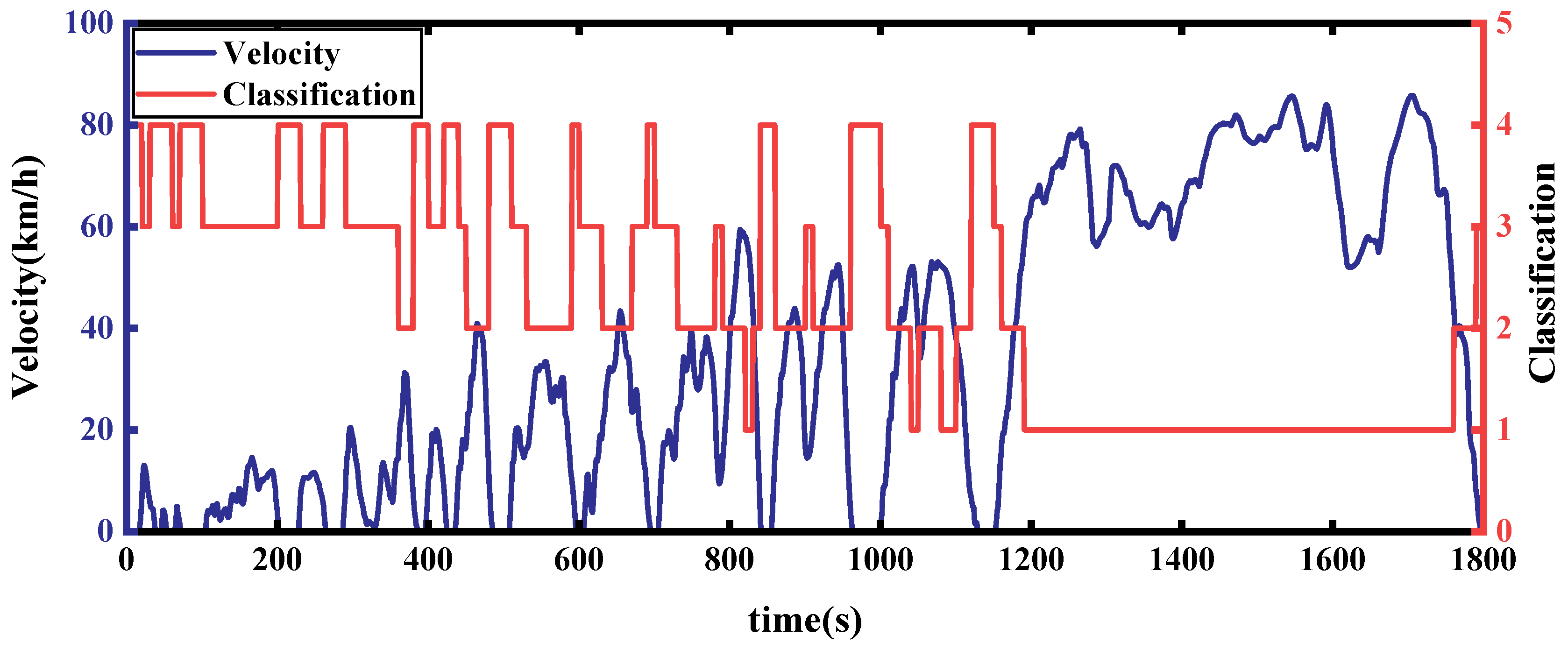
The simulation was carried out at room temperature (20 °C) with a road adhesion coefficient of 0.7 and windless environment. During the simulation, the COA-BPNN identified the characteristic information of the working conditions for 10 s of history, and since the first identification occurred in less than 10 s, the simulated velocity was set to 0 for the first 10 s. Figure 16 shows the results of the working condition identification for the C-WTVC; the red line is the category of a moment identified by the COA-BPNN, where 1, 2, 3, and 4 correspond to highway, suburban, urban smooth, and urban congestion conditions, respectively; the blue line is the vehicle velocity; and the accuracy of the identification results is 97.3%, indicating an almost perfectly accurate recognition.
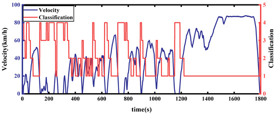
Figure 16.
C-WTVC cycle category recognition effect.
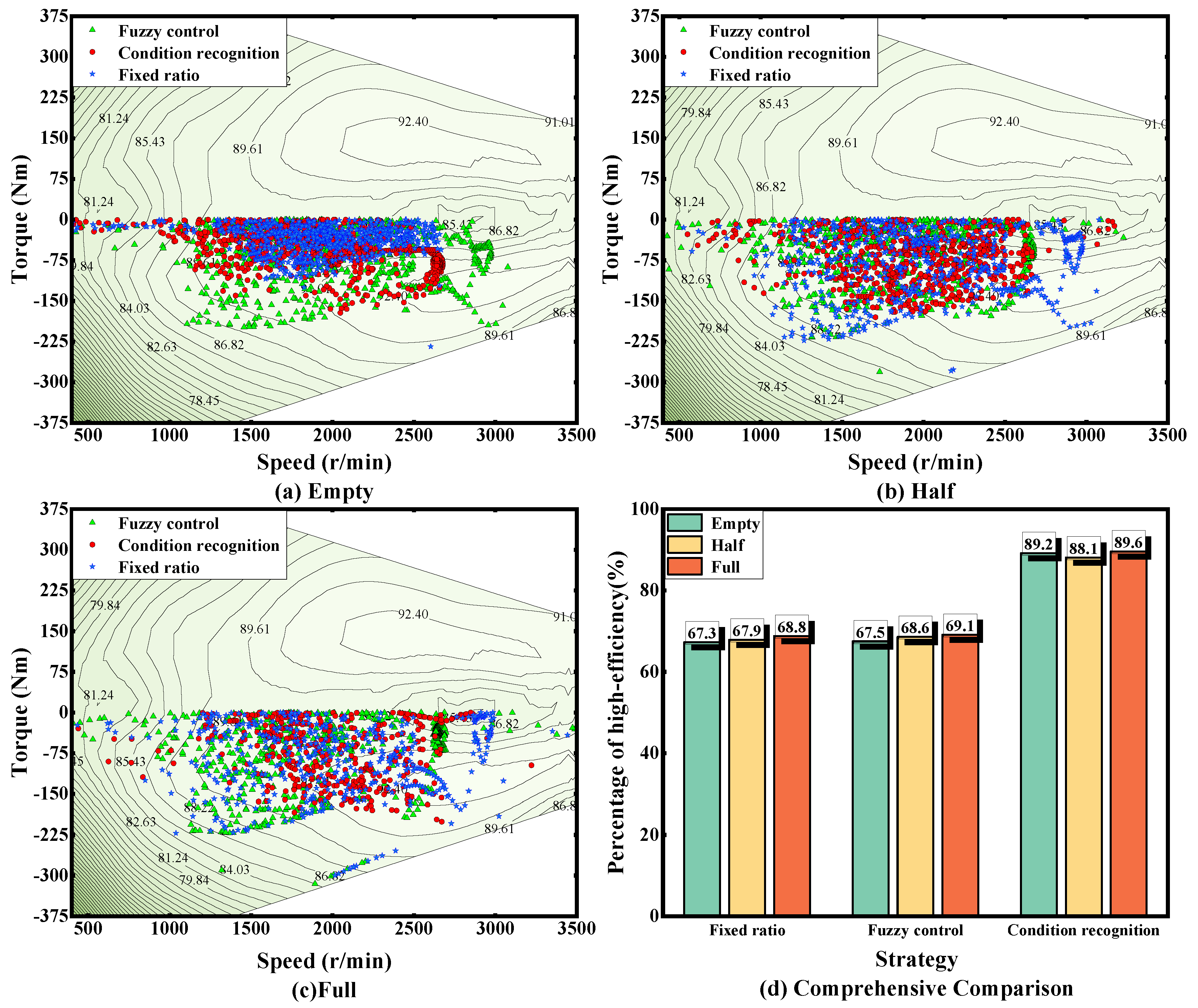
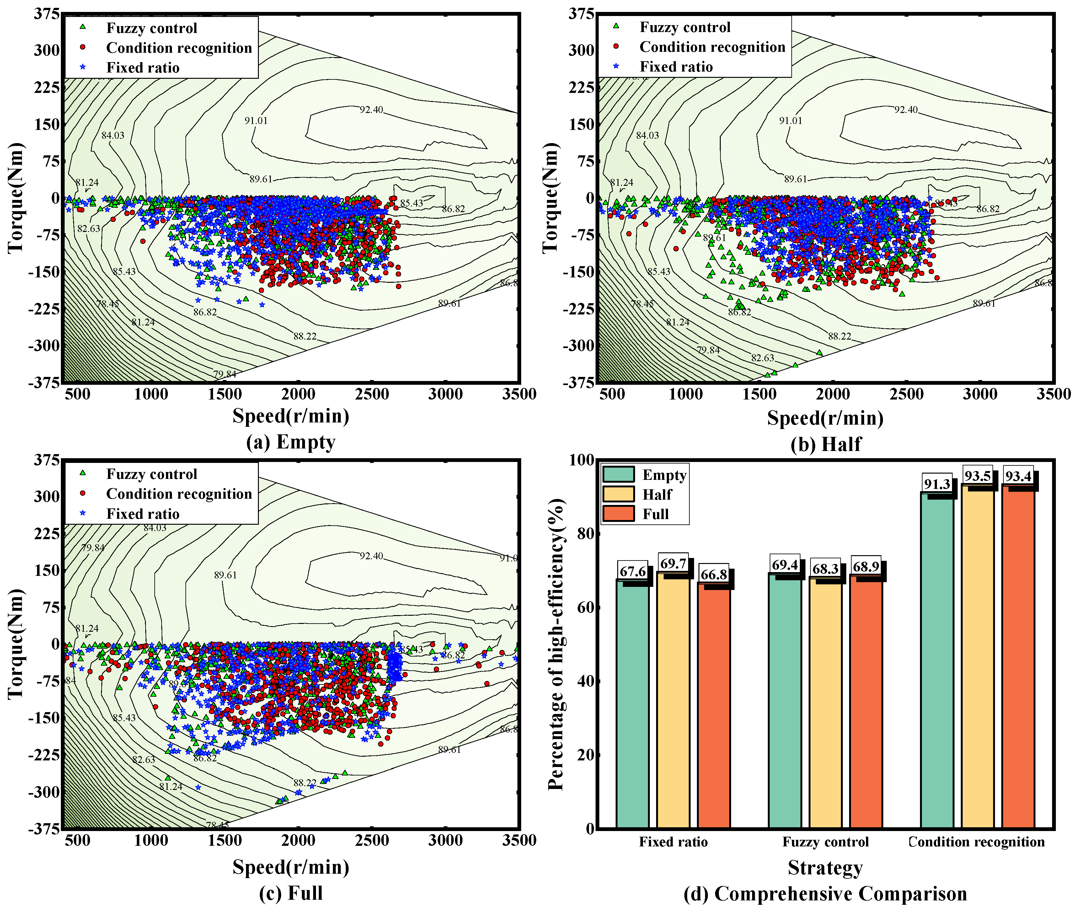
Figure 17 shows the electric motor working points during braking under three loads under C-WTVC conditions, from which it can be clearly seen that the regenerative braking strategy based on the condition identification in this paper is obviously more clustered in the medium- and high-efficiency range during braking, with fewer low-speed and low-torque working points. On the other hand, the electric motor working points are more scattered for the fuzzy control strategy and the fixed-ratio strategy. The period in which the electric motor efficiency is higher than the 89% contour is referred to as the high-efficiency interval. Within this interval, the proportions of the regenerative brake strategy based on condition detection under empty-, half- and full-load states are 89.2%, 88.1%, and 89.6%, respectively; for the fuzzy control strategy, the proportions are 67.5%, 68.6%, and 69.1%, respectively; and for the fixed-ratio strategy, they are 67.3%, 67.9%, and 68.8%, respectively. It can be seen that the regenerative braking strategy based on the identification of the working conditions can effectively limit the electric motor to work in the high-efficiency zone and increase the recovery efficiency.

Figure 17.
Comparison of electric motor working point distribution under C-WTVC conditions.
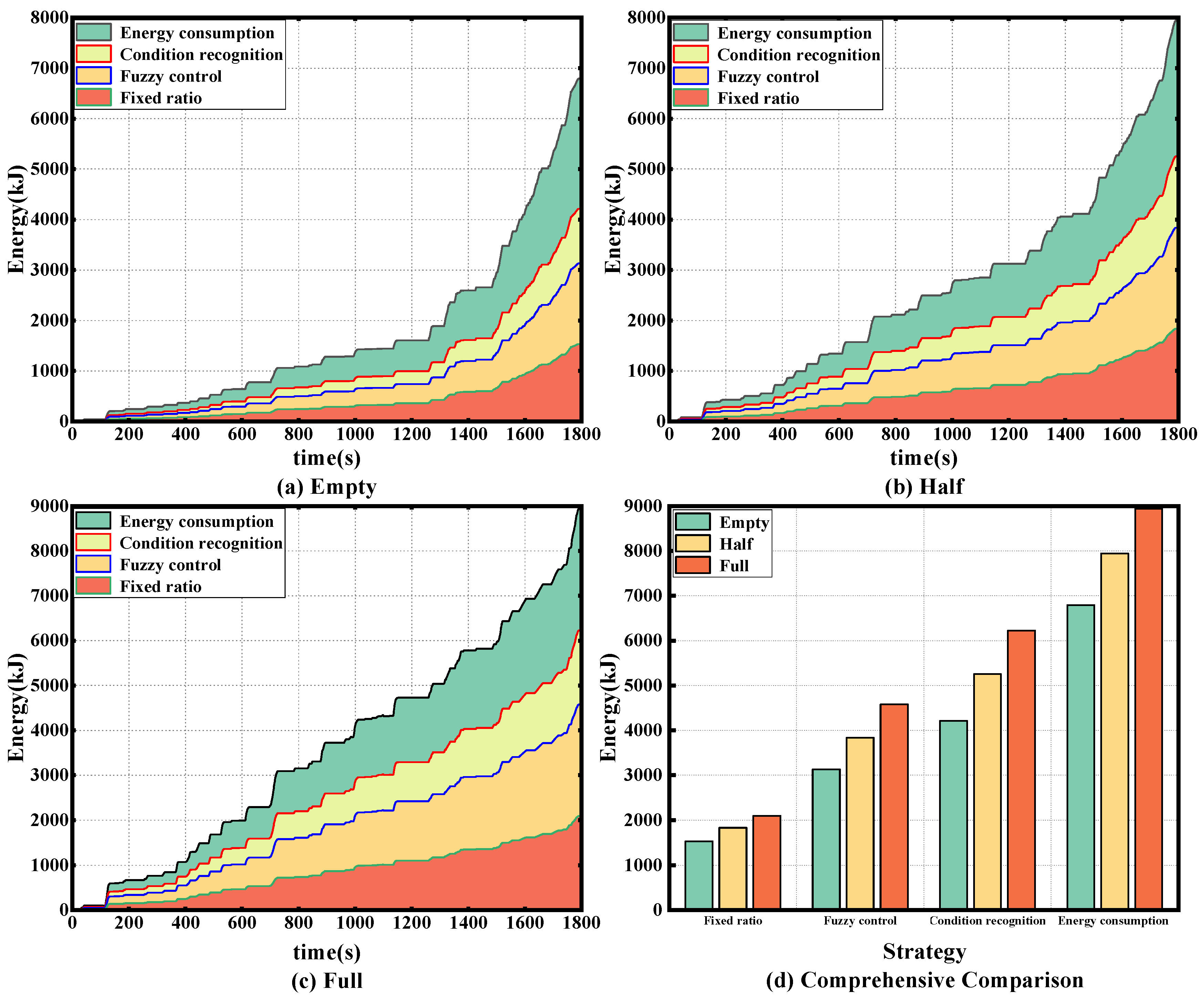
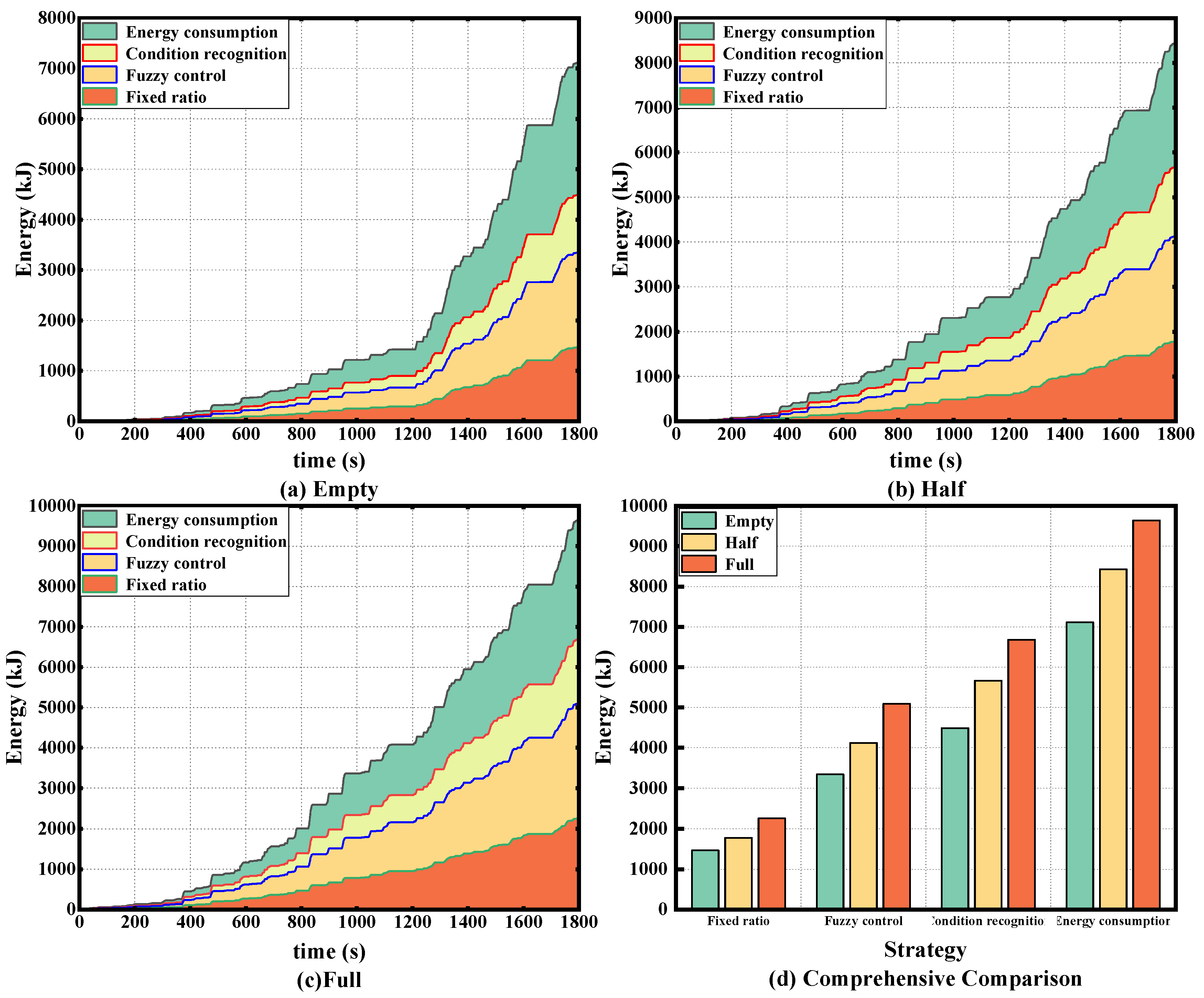
Figure 18 shows a comparison of the total energy consumed and energy recovered from braking for the three load states under the C-WTVC cycle, and it can be clearly seen that, as the load mass of the vehicle rises, the total energy generated during braking increases, and the energy recovered from regenerative braking thus also increases. It is also clear from the graph that the strategy outlined in this paper recovers more energy, regardless of the load.

Figure 18.
Comparison of energy consumed and energy recovered under C-WTVC conditions.
Table 7 shows the simulation results for three kinds of loads under the C-WTVC cycle, from which it can be seen that under empty-, half- and full-load states, the energy recovery rate of this study’s strategy is improved by 34.6%, 36.9%, and 36%, respectively, compared to that observed with the fuzzy control strategy, and the energy recovery rate with the fixed-ratio strategy is improved by 175%, 186.3%, and 197.6%. This indicates that the regenerative braking strategy based on the identification of working conditions can effectively improve the energy recovery rate of the whole vehicle, by ensuring that the braking effect of the whole vehicle is used.
Table 7.
Comparison of simulation results under C-WTVC cycle.
5.2. Comparative Analysis of Simulation under Synthetic Cycle
The synthetic cycle includes urban congestion, urban smooth, suburban, and highway conditions, with more aggressive driving behaviours, including higher rates of acceleration and deceleration. The entire cycle lasts for a total of 1800 s. Figure 19 shows the working condition identification results for the synthetic working conditions in the simulation process, and the accuracy of the identification results is 98.76%.
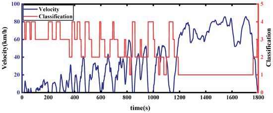
Figure 19.
Synthetic cycle category recognition effect.
Figure 20 shows the working points of the electric motor during braking under synthetic conditions, and it can be seen that, under synthetic conditions, the approximate distribution of the working points is consistent with that of the C-WTVC cycle, indicating that the strategy in this paper is highly adaptable to working conditions.
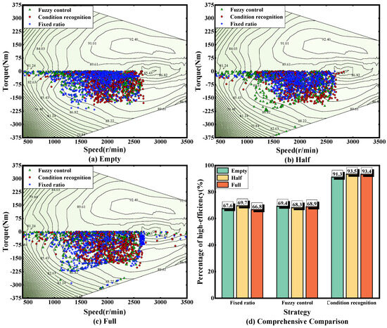
Figure 20.
Comparison of electric motor working point distribution under synthetic conditions.
Figure 21 shows a comparison of the total energy consumed and energy recovered for braking in the three load states under a synthetic cycle, from which it is clear that the strategy of this paper recovers more energy at any load.

Figure 21.
Comparison of energy consumed and energy recovered under synthetic conditions.
Table 8 shows the simulation results for the three loads under synthetic conditions, from which it can be seen that the energy recovery of the strategy in this study was improved by 34.2%, 37.4%, and 31.3% compared with that achieved with the fuzzy control strategy, and by 206.3%, 218.5%, and 197.2% compared with that observed with the fixed-ratio strategy, respectively, under empty, half, and full loads. It can be seen that the regenerative braking strategy based on condition identification resulted in a much higher braking energy recovery than the fuzzy control strategy and the fixed-ratio strategy in both the C-WTVC and synthetic cycles, showing the superiority of the strategy in this paper.
Table 8.
Comparison of simulation results under synthetic conditions.
6. Conclusions
In this paper, we propose a regenerative braking strategy based on condition recognition. First, the whole-vehicle model was built in AVL-Cruise. Second, based on the historical driving data, the historical velocity information was divided into four categories of working conditions with obvious differences, and the COA-BPNN online working condition recognition model was constructed. Third, a GA was used to find the optimal parameters in each category, and the offline parameter library was built; additionally, the COA-BPNN was used to identify the online working conditions and retrieve the corresponding parameters. This strategy considered the influence of the overall vehicle load state and driving conditions on braking, making it more adaptable to working conditions and overall vehicle load, and solved the problem of large changes in geographical and commercial vehicle loads. The constructed COA-BPNN working condition recogniser improved the recognition accuracy by 7.6% compared to the BPNN. The simulation results under C-WTVC and synthetic working conditions show that the energy recovery rate of the strategy proposed in this paper reached up to 69.65%, which is much better than the rates achieved with the fixed-ratio strategy and fuzzy control strategy. In this study, brake force distribution coefficients for different loads were proposed, but the real-time identification of vehicle mass was not considered, so the load change needs to be judged by the driver autonomously, and adaptive mass identification can be added for future research.
Author Contributions
W.Z.: Conceptualisation, Methodology, Data Curation, and Writing—Review and Editing. H.L.: Conceptualisation, Methodology, Simulation, Software, Validation, Investigation, Resources, Data Curation, Writing—Original Draft, and Writing—Review and Editing. J.L.: Conceptualisation, Methodology, and Writing—Review and Editing. All authors have read and agreed to the published version of the manuscript.
Funding
This research was funded by the central guidance for local scientific and technological development funds, grant number Guike ZY23055014; the Innovation-Driven Development Special Fund Project of Guangxi, grant number Guike AA22068060; and the Science and Technology Planning Project of Liuzhou, grant numbers 2022AAA0102 and 2022AAA0104.
Institutional Review Board Statement
Not applicable.
Informed Consent Statement
Not applicable.
Data Availability Statement
The data presented in this study are available on request from the corresponding author. The data are not publicly available due to privacy considerations.
Conflicts of Interest
W.Z., H.L., and J.L. were jointly employed by the Company Commercial Vehicle Technology Center, Dong Feng Liuzhou Automobile Co., Ltd., at the time this study was carried out. The remaining authors declare that the research was conducted in the absence of any commercial or financial relationships that could be construed as potential conflicts of interest.
References
- Guo, Z.; Sun, S.; Wang, Y.; Ni, J.; Qian, X. Impact of New Energy Vehicle Development on China’s Crude Oil Imports: An Empirical Analysis. Electr. Veh. J. 2023, 14, 46. [Google Scholar] [CrossRef]
- Yansong, B.; Khalid, M.; Saifullah; Muhammad, Y.; Saad, D.; Mohsin, A.M.; Ajmal, K.M.; Shah, S.; Khadim, D.; Shah, F.; et al. Global Research on the Air Quality Status in Response to the Electrification of Vehicles. Sci. Total Environ. 2021, 795, 148861. [Google Scholar]
- Ye, C.; Xu, H.; Hu, J.; Peng, Q.; Yang, L. Research on Technology Development Status and Trend Analysis of New Energy Vehicle. IOP Conf. Ser. Earth Environ. Sci. 2020, 558, 052017. [Google Scholar] [CrossRef]
- Squalli, J. Environmental Hypocrisy? Electric and Hybrid Vehicle Adoption and pro-Environmental Attitudes in the United States. Energy 2024, 293, 130670. [Google Scholar] [CrossRef]
- Zhang, P.; Lu, W.; Du, C.; Hu, J.; Yan, F. A Comparative Study of Vehicle Velocity Prediction for Hybrid Electric Vehicles Based on a Neural Network. Mathematics 2024, 12, 575. [Google Scholar] [CrossRef]
- Zhang, H.; Chen, D.; Zhang, H.; Liu, Y. Research on the Influence Factors of Brake Regenerative Energy of Pure Electric Vehicles Based on the CLTC. Energy Rep. 2022, 8, 85–93. [Google Scholar] [CrossRef]
- Yu, Y.; Chao, W.; Shujun, Y.; Xianzhi, T. Study on Top Hierarchy Control Strategy of AEBS over Regenerative Brake and Hydraulic Brake for Hub Motor Drive BEVs. Energies 2022, 15, 8382. [Google Scholar] [CrossRef]
- Geng, C.; Ning, D.; Guo, L.; Xue, Q.; Mei, S. Simulation Research on Regenerative Braking Control Strategy of Hybrid Electric Vehicle. Energies 2021, 14, 2202. [Google Scholar] [CrossRef]
- Jiang, B.; Zhang, X.; Wang, Y.; Hu, W. Regenerative Braking Control Strategy of Electric Vehicles Based on Braking Stability Requirements. Int. J. Automot. Technol. 2021, 22, 465–473. [Google Scholar]
- Yin, Z.; Ma, X.; Zhang, C.; Su, R.; Wang, Q. A Logic Threshold Control Strategy to Improve the Regenerative Braking Energy Recovery of Electric Vehicles. Sustainability 2023, 15, 16850. [Google Scholar] [CrossRef]
- Wei, W.; Chong, G.; Fufan, Q.; Huanhuan, M. Analysis the Effect of Braking Force Distribution Strategy on Energy Recovery Results Considering The Front or Rear Shaft Drives. In Proceedings of the 2019 IEEE 2nd International Conference on Electronic Information and Communication Technology (ICEICT), Harbin, China, 20–22 January 2019; pp. 862–867. [Google Scholar]
- Itani, K.; Bernardinis, A.D.; Khatir, Z.; Jammal, A. Comparison between Two Braking Control Methods Integrating Energy Recovery for a Two-Wheel Front Driven Electric Vehicle. Energy Convers. Manag. 2016, 122, 330–343. [Google Scholar] [CrossRef]
- Sandrini, G.; Gadola, M.; Chindamo, D.; Magri, P. Efficient Regenerative Braking Strategy Aimed at Preserving Vehicle Stability by Preventing Wheel Locking. Transp. Res. Procedia 2023, 70, 28–35. [Google Scholar] [CrossRef]
- El-bakkouri, J.; Ouadi, H.; Giri, F.; Khafallah, M.; Gheouany, S.; Bakali, S.E. Extremum Seeking Based Braking Torque Distribution for Electric Vehicles’ Hybrid Anti-Lock Braking System. IFAC-Paperonline 2023, 56, 2546–2551. [Google Scholar] [CrossRef]
- Li, X. Simulation Analysis of Fuzzy Control Strategy for Braking Energy Recovery of a Pure Electric Vehicle. Int. J. New Dev. Eng. Soc. 2023, 7, 2522–3488. [Google Scholar]
- Yu, Z.; Feng, H.; Meng, Y.; Xu, E.; Wu, Y. Braking Energy Management Strategy for Electric Vehicles Based on Working Condition Prediction. AIP Adv. 2022, 12, 015220. [Google Scholar] [CrossRef]
- Li, W.; Xu, H.; Liu, X.; Wang, Y.; Zhu, Y.; Lin, X.; Wang, Z.; Zhang, Y. Regenerative Braking Control Strategy for Pure Electric Vehicles Based on Fuzzy Neural Network. Ain Shams Eng. J. 2024, 15, 102430. [Google Scholar] [CrossRef]
- Mei, P.; Karimi, H.R.; Yang, S.; Xu, B.; Huang, C. An Adaptive fUzzy Sliding-mode Control for Regenerative Braking System of Electric Vehicles. Int. J. Adapt. Control Signal Process 2021, 36, 391–410. [Google Scholar] [CrossRef]
- Li, L.; Zhang, Y.; Yang, C.; Yan, B.; Martinez, C.M. Model Predictive Control-Based Efficient Energy Recovery Control Strategy for Regenerative Braking System of Hybrid Electric Bus. Energy Convers. Manag. 2016, 111, 299–314. [Google Scholar] [CrossRef]
- Haspolat, C.; Yalcin, Y. Energy Management of P2 Hybrid Electric Vehicle Based on Event-Triggered Nonlinear Model Predictive Control and Deep Q Network. World Electr. Veh. J. 2023, 14, 135. [Google Scholar] [CrossRef]
- Liu, Y.; Gene, L.Y.; Chia, L.M. Fuel Economy Improvement and Emission Reduction of 48 V Mild Hybrid Electric Vehicles with P0, P1, and P2 Architectures with Lithium Battery Cell Experimental Data. Adv. Mech. Eng. 2021, 13, 16878140211036022. [Google Scholar] [CrossRef]
- Wang, X.; Liu, S.; Ye, P.; Zhu, Y.; Yuan, Y.; Chen, L. Study of a Hybrid Vehicle Powertrain Parameter Matching Design Based on the Combination of Orthogonal Test and Cruise Software. Sustainability 2023, 15, 10774. [Google Scholar] [CrossRef]
- Guo, S.; Wu, K.; Zhang, G. Application of PCA-K-Means++ Combination Model to Construction of Light Vehicle Driving Conditions in Intelligent Traffic. J. Meas. Eng. 2020, 8, 107–121. [Google Scholar] [CrossRef]
- Chunna, L.; Yan, L. Energy Management Strategy for Plug-In Hybrid Electric Vehicles Based on Driving Condition Recognition: A Review. Electronics 2022, 11, 342. [Google Scholar] [CrossRef]
- Dapai, S.; Shipeng, L.; Kangjie, L.; Yinggang, X.; Yun, W.; Changzheng, G. Adaptive Energy Management Strategy for Plug-in Hybrid Electric Vehicles Based on Intelligent Recognition of Driving Cycle. Energy Explor. Exploit. 2023, 41, 246–272. [Google Scholar]
- Wang, P.; Gu, T.; Sun, B.; Dang, R.; Wang, Z.; Li, W. Energy Management of Electromechanical Flywheel Hybrid Electric Vehicle Based on Condition Prediction. Eng. Lett. 2022, 30, EL_30_4_11. [Google Scholar]
- Yang, F.; Liu, S.; Dobriban, E.; Woodruff, D.P. How to Reduce Dimension with PCA and Random Projections? IEEE Trans. Inf. Theory 2021, 67, 8154–8189. [Google Scholar] [CrossRef]
- Rustam, M.; Nenad, M.; Bassem, J.; Ravil, M. How to Use K-Means for Big Data Clustering? Pattern Recognit. 2023, 137, 109269. [Google Scholar]
- Upendra, K. A Noval Approach for Object Recognition Using Decision Tree Clustering by Incorporating Multi-Level BPNN Classifiers and Hybrid Texture Features. Int. J. Inf. Retr. Res. 2024, 14, 1–31. [Google Scholar]
- Mohammad, D.; Zeinab, M.; Eva, T.; Pavel, T. Coati Optimization Algorithm: A New Bio-Inspired Metaheuristic Algorithm for Solving Optimization Problems. Knowl. Based Syst. 2023, 259, 110011. [Google Scholar]


Disclaimer/Publisher’s Note: The statements, opinions and data contained in all publications are solely those of the individual author(s) and contributor(s) and not of MDPI and/or the editor(s). MDPI and/or the editor(s) disclaim responsibility for any injury to people or property resulting from any ideas, methods, instructions or products referred to in the content. |
© 2024 by the authors. Licensee MDPI, Basel, Switzerland. This article is an open access article distributed under the terms and conditions of the Creative Commons Attribution (CC BY) license (https://creativecommons.org/licenses/by/4.0/).