1. Introduction
With the increase in car ownership, the environmental pressure caused by conventional-fuel vehicles is becoming ever more apparent, with a significant impact on the global environment [
1,
2]. Hybrid vehicles are a model for the transition from traditional-fuel vehicles to pure electrification and are currently the most promising models in the transport electrification industry [
3,
4].
Hybrid vehicles have two power sources—the combustion engine and the electric motor—so their advantage lies in the fact that their energy utilisation efficiency can be maximised through energy management strategies, and the electric motor can be used as a generator to recover braking energy. Commercial vehicles generate more braking energy due to their larger mass, making the recovery of this braking energy even more important [
5].
The usual brake force distribution strategy is a front and rear axle brake force distribution, as well as mechanical braking of the drive axle, and an electric machine power distribution strategy. A balanced distribution of the electromechanical brake force between the front and rear axles is crucial for energy recovery [
6,
7].
In research on front and rear axle brake force distribution, many scholars use different strategies to distribute the brake force between the front and rear axles. Geng C et al. [
8] proposed a zigzag distribution curve combining the I curve, the f-group line (the front and rear brake force distribution line in the case of only the front wheels locking or the front wheels locking first), and the ECE regulation curve based on the brake intensity. Jiang B et al. [
9] proposed a variable-ratio brake force distribution strategy for the front and rear axle, based on brake intensity, to find the optimal brake force distribution coefficient β, to improve energy recovery efficiency. Yin.Z et al. [
10] set three thresholds for the battery state of charge (SOC), velocity, and braking intensity. This approach allows the front and rear axle braking force distribution to be reclassified, improving braking safety and significantly enhancing braking energy recovery effectiveness. Wei W et al. [
11] proposed a braking energy maximisation control strategy, setting three braking intensity thresholds corresponding to three braking force allocation strategies. Itani K et al. [
12] proposed a sliding mode controller to regulate the sliding film ratio of wheel braking, effectively improving the braking stability of the whole vehicle; however, due to the over-assurance of stability, this approach led to low energy recovery. Sandrini G [
13] proposed a regenerative braking logic for front-wheel drive (FWD), rear-wheel drive (RWD) or all-wheel drive (AWD) use. El-bakkouri J et al. [
14] proposed an objective and constraints for the braking torque distribution of a hybrid anti-lock braking system (ABS) based on the extreme search technique, which constitutes a better treatment. Regenerative energy is maximised, and the battery’s state of charge is improved, by optimising the electric braking system’s efficiency.
In their research on driving axle mechanical and electric motor brake force distribution, many scholars use algorithmic optimisation or fuzzy control to find the optimal distribution coefficient trajectory. Li X et al. [
15] used a fuzzy control strategy to design a brake energy recovery strategy with the braking intensity, velocity, and SOC as inputs and electromechanical brake power distribution coefficients as outputs. The simulation results show that the method effectively improves the energy recovery rate. Zhai Y et al. [
16] used historical 100 s driving information to predict velocity in a future period, to determine the optimum dual-motor torque distribution under the predicted operating conditions to improve energy recovery. Li W et al. [
17] proposed a fuzzy control strategy considering braking intensity, and the simulation results showed that the energy recovery rate reached 39.6%. Mei P et al. [
18] proposed an adaptive fuzzy control strategy, wherein a genetic algorithm was used to determine the optimal allocation parameters, and the strategy also incorporated the driver’s influence on the weight factor to achieve dynamic control. Li L et al. [
19] optimised the torque distribution across the regenerative braking system, and the mechanical braking system was optimised using a particle swarm optimisation algorithm.
In summary, research on brake energy recovery technology for the passenger car sector has shown some progress, but there is still limited-application research in the commercial vehicle sector. Due to the large mass variation in commercial vehicles, which are primarily rear-driven, the established recovery strategies are relatively simplistic, leading to low energy utilisation, poor braking smoothness, and little consideration of the effects of working conditions and loads on braking safety and energy recovery efficiency. As a result, these strategies cannot be effectively applied to scenarios encountered in the actual driving process. In real driving situations, emergencies sometimes occur, and the existing strategies are ambiguous regarding whether energy recovery should be performed when braking is intense. The safety of braking should be fully considered during emergency braking, when all of the braking force needs to be provided by the mechanical brake, without regenerative braking, to ensure that the car can stop quickly.
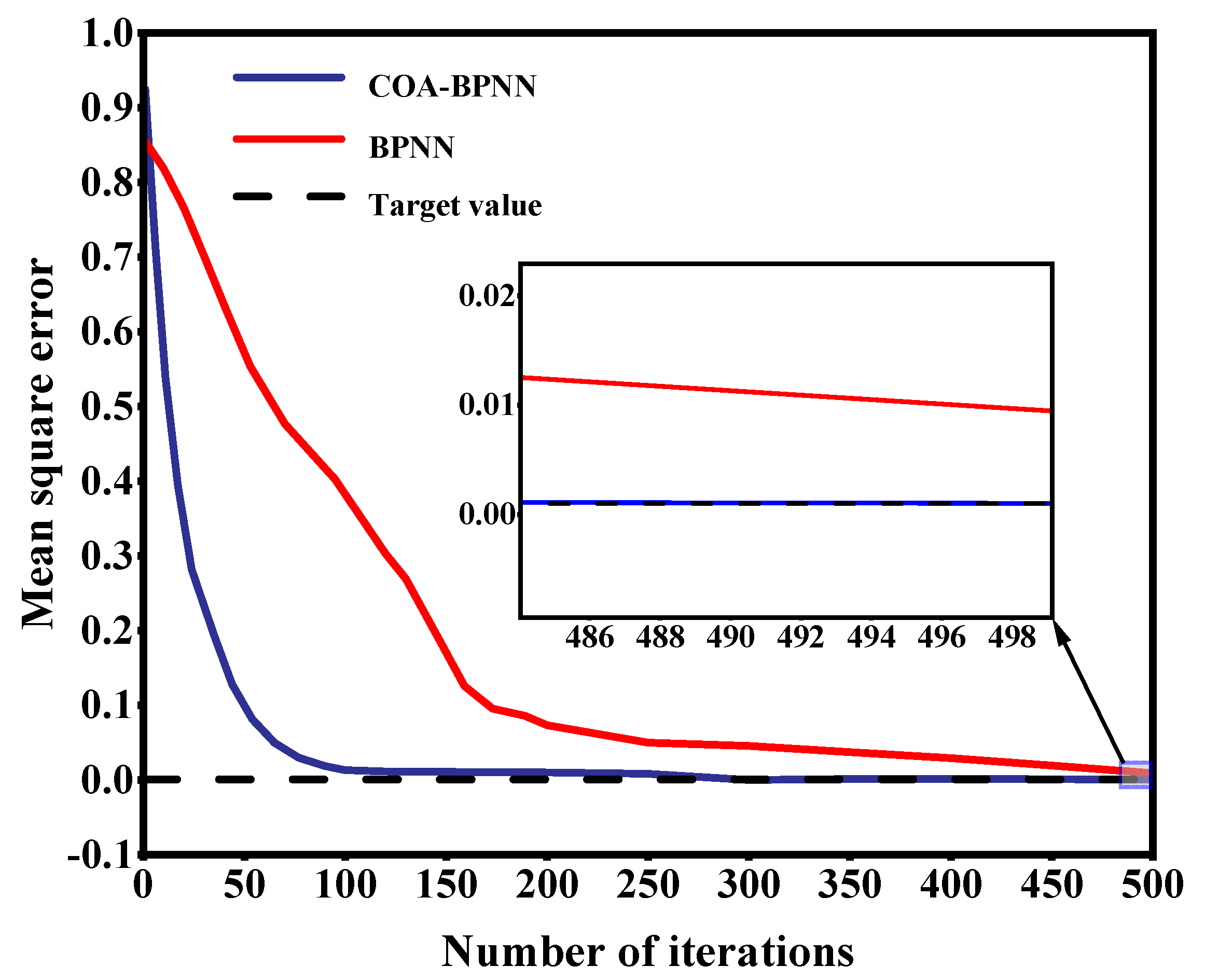
Aiming to address the above problems in brake energy recovery strategies for commercial vehicles, this paper proposes a strategy based on the identification of working conditions. Firstly, taking into account the effect of braking in the whole vehicle load state, the strategy of distributing the braking force of the front and rear axles in the empty-, half- and full-load states is proposed, according to the braking intensity magnitude and load state. Secondly, according to the GPS data on the historical driving data of commercial vehicles, and according to the performance parameter indicators of the vehicle, and the time–velocity sequence of data pre-processing, the use of pre-processed data, through the Coati optimisation algorithm (COA), was used for the optimisation of the back propagation neural network (BPNN) to construct the working condition identifier. Finally, a genetic algorithm was used to determine the optimal control parameters of the three loads under each working condition category, and the COA-BPNN working condition identifier identified the current working condition category to retrieve the corresponding optimal control parameters in the offline parameter library.
The paper is structured as follows: In
Section 2, the whole-vehicle model of a hybrid commercial vehicle is introduced, and its construction in AVL-Cruise v.2019 software is described. In
Section 3, the data processing, state classification, and state recognition construction are presented. In
Section 4, the development of front and rear axle brake power distribution strategies, based on different loads and energy recovery strategies based on state recognition, is described, as is the construction of the strategy model in Simulink. In
Section 5, the simulation of the strategies is described, and the results are studied. In
Section 6, conclusions are drawn.
2. HEV Model
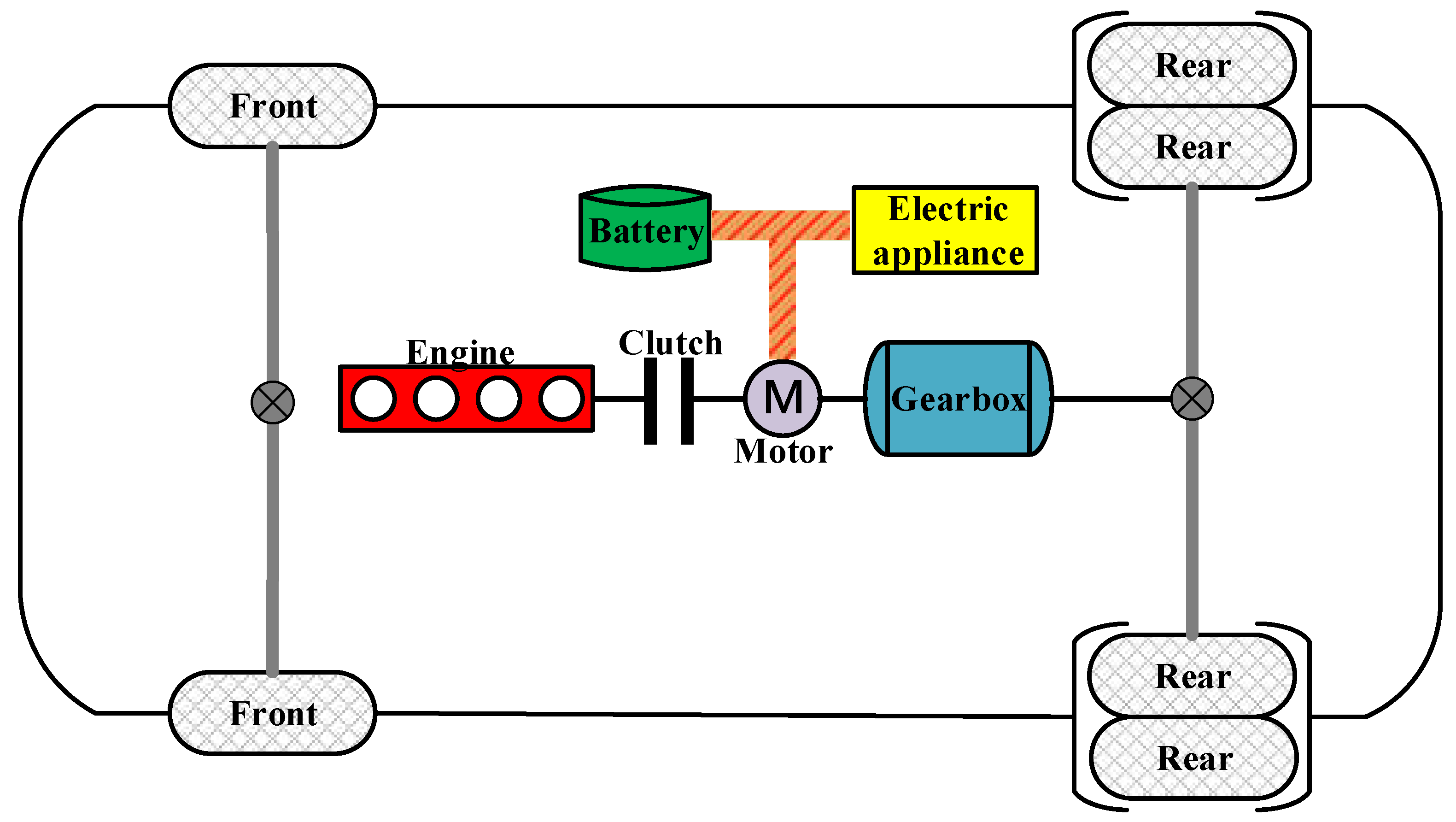
In this study, the P2 hybrid commercial vehicle was selected as the model, and its topology is shown in
Figure 1. The electric motor of the P2 hybrid vehicle is located between the combustion engine and the transmission, and the torque coupling between the electric motor and the combustion engine is controlled by the clutch, so that different vehicle control and energy management strategies can be set, to achieve different driving modes and improve the overall vehicle dynamics and fuel economy [
20]. With the rapid development of new energy vehicles, the P2 structure has been widely adopted by major manufacturers due to its low cost [
21].
Table 1 shows the vehicle parameters of the hybrid vehicle.
2.1. Vehicle Model
When a car travels, it must overcome rolling resistance, air resistance, gradient resistance, and acceleration resistance; thus, the following equation for the car’s movement can be formed:
where
is the driving force, and it can be expressed in terms of:
where
is the combustion engine torque;
is the transmission ratio;
is the main transmission ratio;
is the transmission efficiency;
is the tyre radius;
is gravity;
is the tyre rolling resistance coefficient;
is the slope angle;
is the air resistance coefficient;
is the upwind area;
is the car velocity;
is the mass conversion coefficient; and
is the total mass of the car.
2.2. Combustion Engine Parameter Matching
The performance of the car cannot be sacrificed when improving its economy. The performance index for a car is assessed using the maximum speed
, acceleration time
and maximum gradient climb
[
22]. Regarding the pure combustion engine drive, when the car is at maximum velocity under the demand power
and the maximum gradient-climbing demand power
needed to produce the total combustion engine power
, both need to satisfy the following formula:
where
is the total combustion engine power at the maximum velocity;
is the maximum velocity;
is the transmission efficiency;
is the unladen mass;
is the rolling resistance coefficient;
is the air resistance coefficient;
is the windward area of the vehicle; and
is the demanded power of the high voltage appliance, which takes the value 10%
.
- 2.
The total power is calculated based on the maximum gradient climbed.
where
is the velocity when climbing the slope;
is the full-load mass;
is the maximum climbing angle,
,
; and
takes the value 10%
.
In summary, the main combustion engine parameters are obtained, as shown in
Table 2:
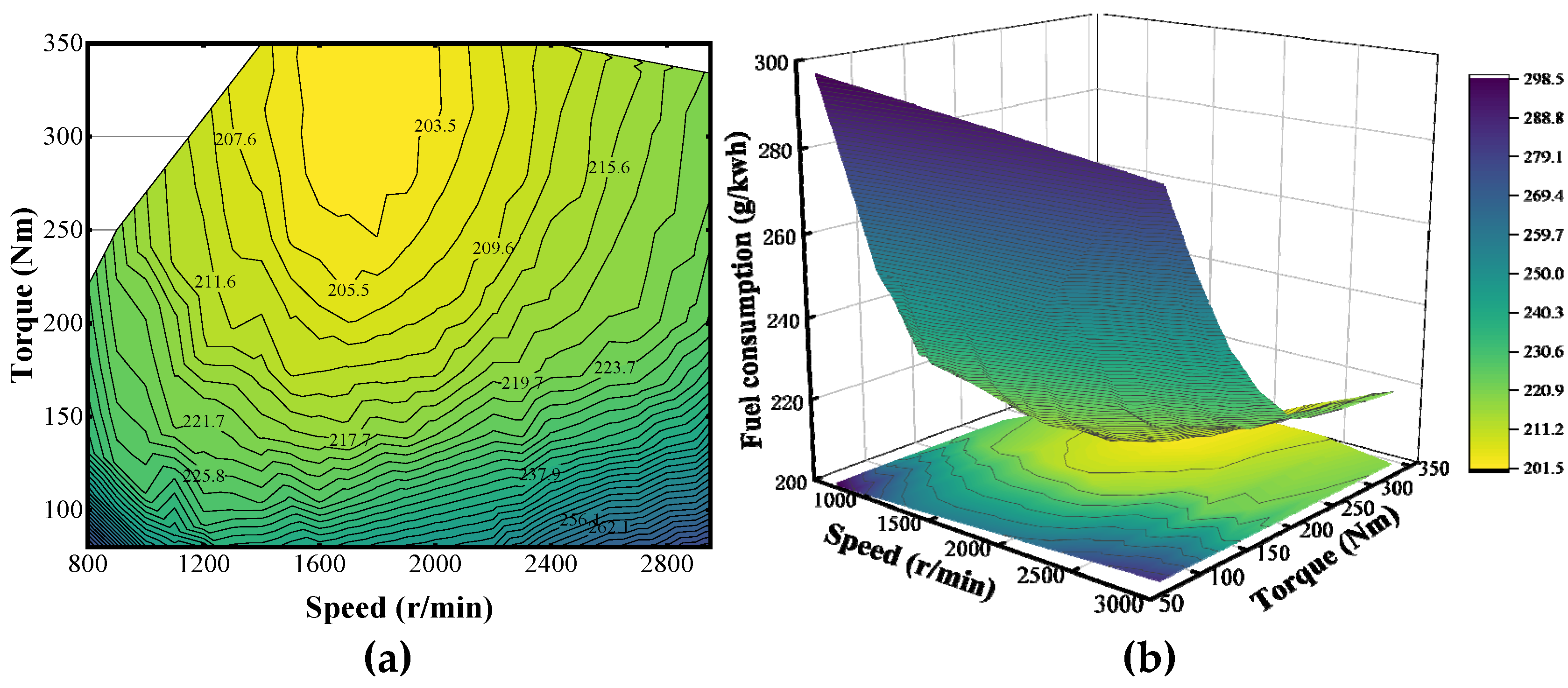
Two- and three-dimensional contour maps of the combustion engine are shown in
Figure 2.
2.3. Electric Motor Parameter Matching
When the electric motor is driven alone, it is necessary to simultaneously satisfy the demand power at maximum velocity in EV mode, the demand power at the maximum gradient climb, and the demand power at maximum acceleration, where and should be kept equal to the electric motor parameters.
Neglecting the gradient resistance, the electric motor power demand
is calculated from the maximum acceleration as:
where
is the final velocity of acceleration, km/h;
is the total time of acceleration, s; and
is the fitting coefficient, taken as 0.5.
The maximum electric motor speed is calculated using the following formula:
The electric motor rated speed is calculated using the formula:
where
is the maximum velocity;
is the main deceleration ratio;
is the tyre radius; and
is the expanded constant power zone coefficient, which takes the value of 2.
The torque of the electric motor can be obtained from Equation (9).
In summary, the main electric motor parameters are obtained, as shown in
Table 3.
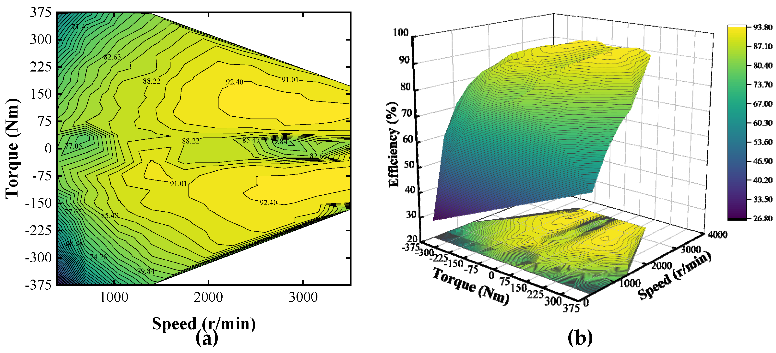
Two- and three-dimensional efficiency maps of the electric motor are shown in
Figure 3.
2.4. Power Battery Models
The power battery is mainly used to provide power to the electric motor; taking into account the role of energy recovery, the battery pack in this study consisted of 550 single lithium batteries. The relationship between the
rate of change and the current is as follows:
The capacity of the power battery pack can be calculated based on the nationally specified range, the target constant velocity, and the power requirement of the electric motor. The capacity requirement for the power battery pack for the target range is:
where
is the uniform velocity;
is the target driving range;
is the working efficiency of the electric motor;
is the voltage of the power battery pack; and
is the power required by the electric motor.
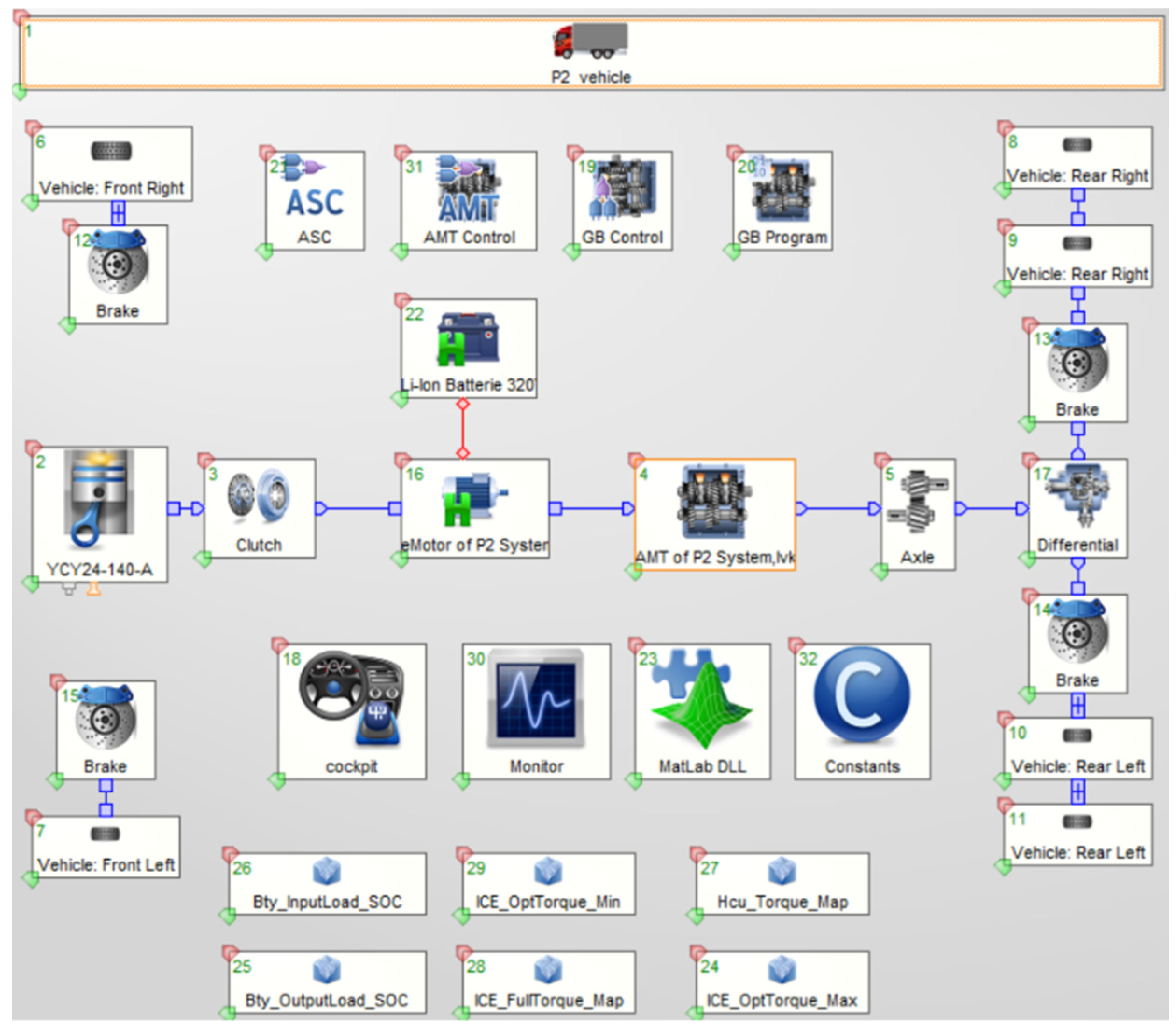
2.5. Vehicle Model Construction
AVL-Cruise v.2019 is a piece of software developed by AVL for the power components of the whole vehicle; it can be used to study the fuel consumption and dynamics of different vehicles under different working conditions. The way the software divides the whole vehicle into several small modules makes it easy for the user to build different vehicle models according to their own ideas, and its complete solver can quickly output accurate results; therefore, AVL-Cruise v.2019 software was used in this study, and whole-vehicle modelling was carried out based on the topology of the P2 hybrid vehicle as described in the previous section. The specific steps are as follows:
Step 1: According to the structure of the P2 hybrid vehicle, build the mechanical connection model between the vehicle, wheels, combustion engine, electric motor, clutch, transmission, brake, power battery, main reduction gear, and differential, etc., in Cruise.
Step 2: Enter the basic parameters of the whole vehicle and the parameters of the selected components.
Step 3: Set the mechanical and electrical connections, outputs, and output signals between the components.
Figure 4 shows the Cruise vehicle model created in this study.
4. Construction of Regenerative Brake Strategy Based on Condition Identification
This section describes how a distribution strategy was designed to develop the front and rear axle braking force distribution coefficients as a variable ratio value, based on the no-load, half-load and full-load braking force. Then, based on the six key control parameters affecting the electric motor braking energy recovery efficiency, each category of working conditions derived from the clustering in
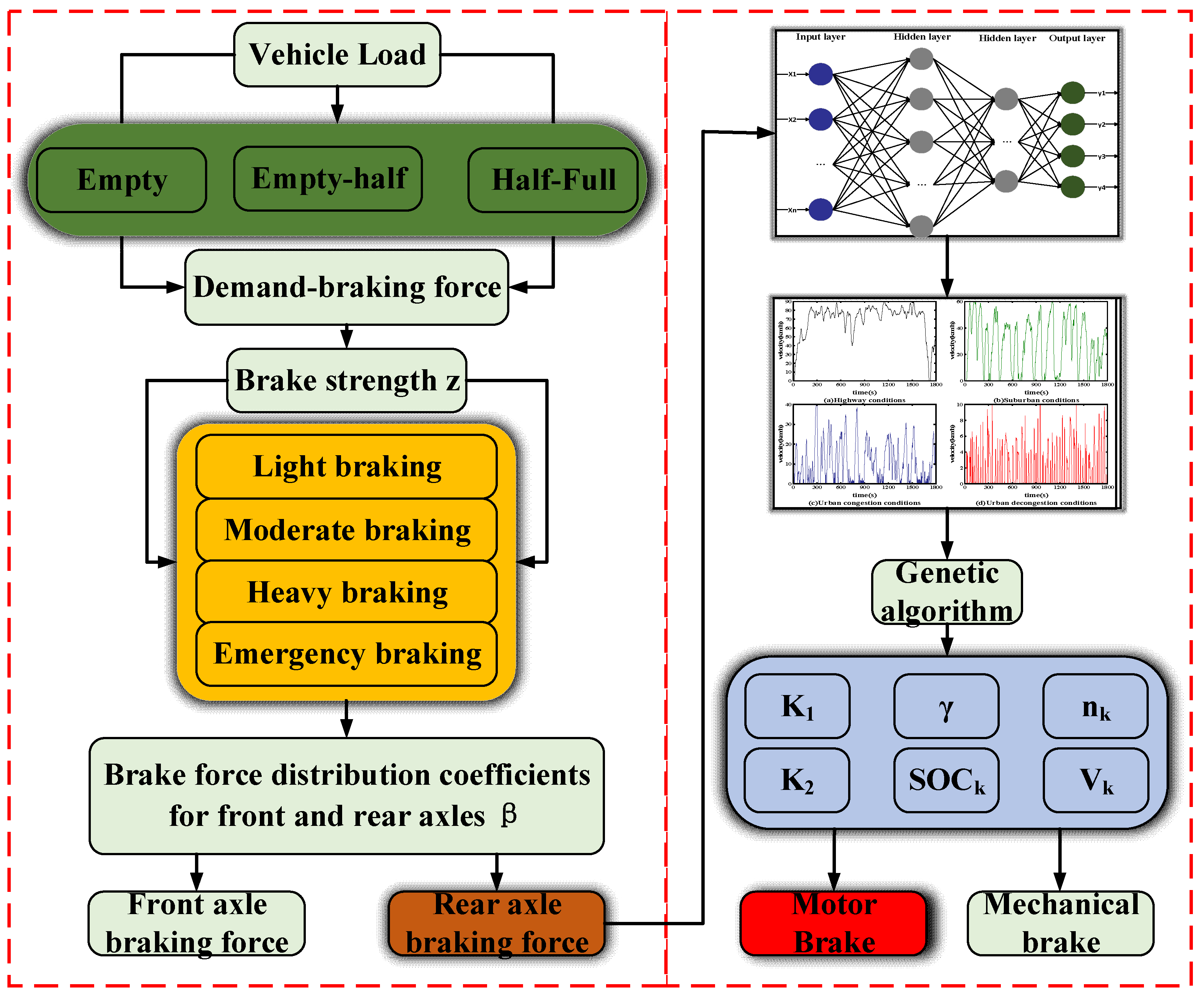
Section 3 was individually treated as a working condition velocity, and a genetic algorithm was used to determine the optimal control parameters for the three kinds of loads under each category of working conditions; then, through the COA-BPNN online working condition recogniser, the algorithm identified the current category of working conditions and retrieved the corresponding optimal control parameters in the offline parameter library, and the electric motor demand braking force and mechanical braking force were calculated.
Figure 11 shows the framework of the condition recognition-based regenerative braking strategy.
4.1. Front and Rear Axle Brake Force Distribution Strategy
4.1.1. Front and Rear Axle Brake Force Distribution Curve Analysis
In the braking process, when the braking force can meet the vehicle braking conditions, the front and rear wheels exhibit the following three states: first, the front wheels take the lead in holding and slipping; second, the rear wheels take the lead in holding and slipping; third, the front and rear wheels are simultaneously responsible for holding and slipping. These are the most ideal conditions, as they can avoid rear axle side slip, ensuring the best utilisation rate for adhesion under these conditions, thereby meeting the requirements of vehicle braking safety and stability. At this point, both the front and rear wheels can be in an ideal state of holding dead simultaneously. This occurs when the front and rear axle braking force distribution curve forms what is referred to as an
curve. The formula for the ideal braking relationship function between the front and rear axle braking forces is as follows:
where
is the front axle brake force;
is the rear axle brake force;
is the wheelbase of the vehicle;
is the gravitational force of the vehicle;
is the height of the centre of mass of the vehicle; and
is the distance from the rear axle to the centre of mass of the vehicle.
- 2.
ECE regulation requirements
For lorries with a gross mass of more than 3.5 tonnes, the UNECE braking regulation ECER13 sets out requirements for the distribution of braking force between the front and rear axles of such vehicles. The distribution of braking force between the front and rear axles is expressed by the braking force distribution coefficient
, i.e., the ratio of the braking force of the front axle and the total braking force required by the vehicle. According to an analysis of the regulation, the front and rear axle brake force distribution coefficient
and the braking intensity are defined as follows:
4.1.2. Front and Rear Axle Brake Force Distribution Strategy
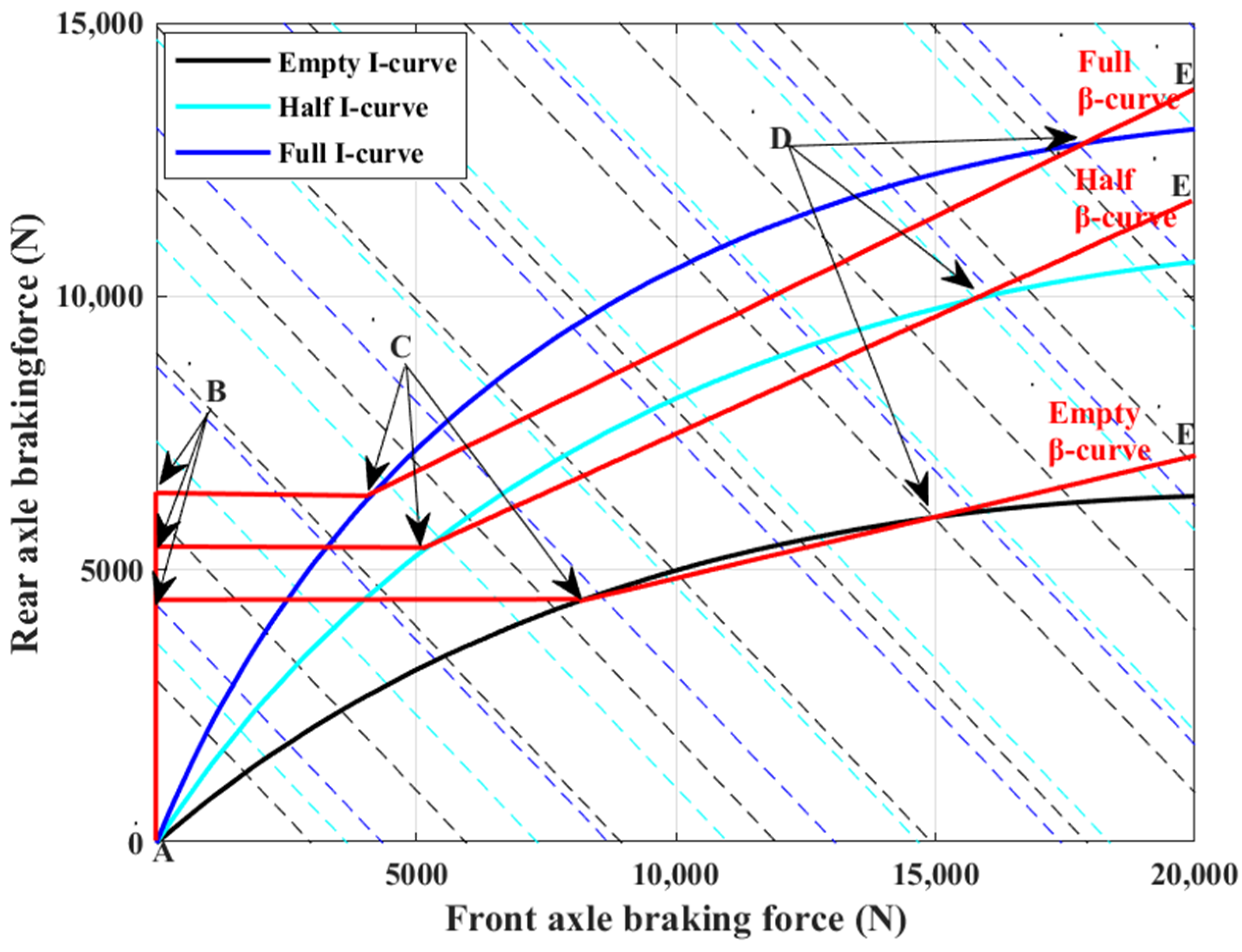
According to the level of braking intensity, braking is divided into four modes: light, medium, heavy, and emergency braking. As the rear wheel first locking in the braking process represents an unstable condition, an empty-, half-, and full-load/front- and rear-axle braking force distribution strategy was developed, based on the comprehensive consideration of the f-group line (the front wheel first locking and the rear wheel not being wrapped), ECE braking regulations, and the ideal braking force distribution curve of different loads. Brake force distribution curves for the front and rear axles are shown in
Figure 12.
As shown in
Figure 12, the brake force distribution rules are as follows:
- (1)
Light braking mode: When the braking intensity is between 0 and 0.15 (), regardless of the current vehicle load, all of the braking force is distributed to the rear axle according to the AB curve. The maximum braking force is provided by the electric motor, and the mechanical brake plays a complementary role.
- (2)
Medium braking mode: The vehicle distributes the braking force according to the BC curve, the braking force of the rear axle remains unchanged, and the braking force of the front axle increases linearly with the increase in braking intensity, until the no-load threshold , half-load threshold , and full-load threshold are reached.
- (3)
Hard braking mode: The vehicle distributes the brake force along the CD curve, and the brake force distribution curve is always below the ideal brake force distribution coefficient curve and close to the I curve, until it coincides again with the ideal brake force distribution coefficient curve, at which point .
- (4)
Emergency braking mode: If , no regenerative braking is performed under any load condition, and the braking force is fully distributed to the mechanical brakes of the front and rear axles, according to the DE curve.
4.2. Optimisation of Regenerative Braking Parameters Based on GA
The efficiency of regenerative braking energy recovery is mainly affected by the vehicle velocity, battery charge state, battery charging power, electric motor characteristics, and the ratio of brake force distribution between mechanical and electric motor; the braking torque requirement of the electric motor can be calculated using the following equation:
where
is the vehicle demand brake torque;
is the electric motor brake demand torque;
is the velocity correction factor;
is the
correction coefficient;
is the transmission efficiency;
is the electric motor brake demand torque gain coefficient; and
is the mechanical and electric motor brake force distribution coefficient, i.e., the ratio of the electric motor brake torque to the total brake torque of the rear axle.
When
, the battery limits the maximum charge power to limit the power generated by the electric motor, thus extending the life of the battery.
where
is the generating power of the electric motor;
is the maximum charging power of the battery; and
is the maximum charging power gain coefficient of the battery.
The electric motor speed affects the efficiency of the electric motor’s power generation, and the regenerative braking minimum electric motor speed keeps the electric motor in a more efficient working range.
where
is the power at minimum speed and
is the minimum speed of regenerative braking, in rpm.
In this study, the velocity correction factor was set within the range [0.8, 1.2]; the battery SOC correction factor was set within the range [0.8, 1.2]; the electric motor braking demand torque gain coefficient was set within the range [1, 4]; the maximum battery charging power amplification coefficient was set within the range [0.5, 1]; the minimum speed of the electric motor for regenerative braking was set within the range [400, 800]; and the mechanical and electric motor braking force distribution coefficients were optimised in the range [0, 1] to obtain the best regenerative braking energy recovery efficiency.
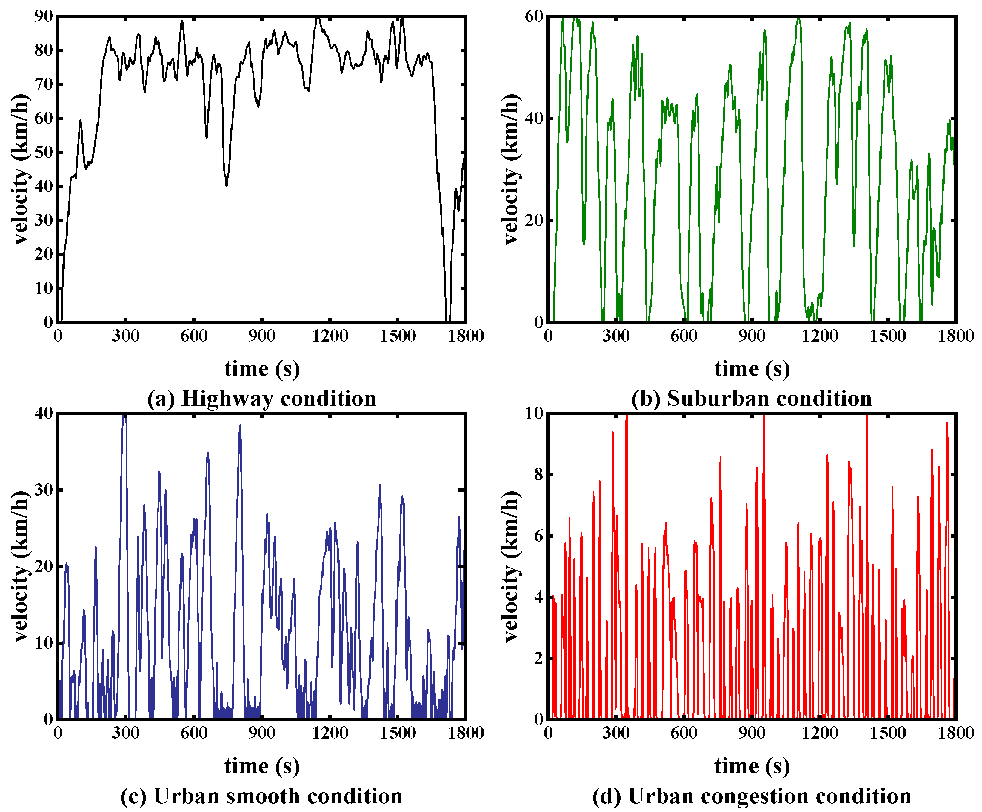
Four driving conditions were defined and obtained, as described in
Section 3;
Figure 13 shows some of the time–velocity curves synthesised for the four conditions, where (a), (b), (c), and (d) were synthesised using only kinematic segments of the highway, suburban, urban smooth, and urban congestion working conditions, respectively, and parameter optimisation was performed under each of the four conditions.
The genetic algorithm (GA) is an adaptive global search method for finding optimal solutions through the simulation of the evolutionary process, which defines the search space of optimal solutions as an evolutionary process and solves them with a set of stochastic rules. GAs do not have the restriction of the hard rules found in traditional algorithms, giving them superior parallel solving abilities and global optimality search abilities, and they can also effectively solve multi-objective optimisation problems; therefore, a GA was chosen for offline parameter determination in this study. The steps of the GA used in this study for parameter optimisation were as follows:
Step 1: The target parameters and their constraints were determined, and the six control parameters were formed into an individual component of the genetic algorithm.
Step 2: The target working conditions and the target load state were determined. The four synthetic working conditions clustered above were used to run the strategy separately, to derive the optimal control parameters under different working conditions.
Step 3: Coding and population initialisation. The binary coding method was used to encode the six control parameters into individuals; the random method was used to initialise the population.
Step 4: Setting and calculating the fitness function. Considering the brake energy recovery efficiency and brake safety, the sum of the minimum brake energy loss and brake safety was selected as the objective function, as shown in Equation (25).
where
decreases as the braking intensity becomes larger, and vice versa for
. Equation (26) is the weighting factor rule.
Step 5: According to the degree of adaptation of the individual determining the probability of the individual to be selected, the better the adaptation of the individual, the greater is the probability of being selected.
Step 6: If the value of the objective function satisfies the condition or reaches the maximum number of iterations, then stop the iteration and output the optimal value; if it does not satisfy the condition, then return to Step 4.
Table 6 shows the values of the optimum control parameters for different loads, obtained according to the above steps.
4.3. Regenerative Braking Strategy Modelling Based on Condition Identification
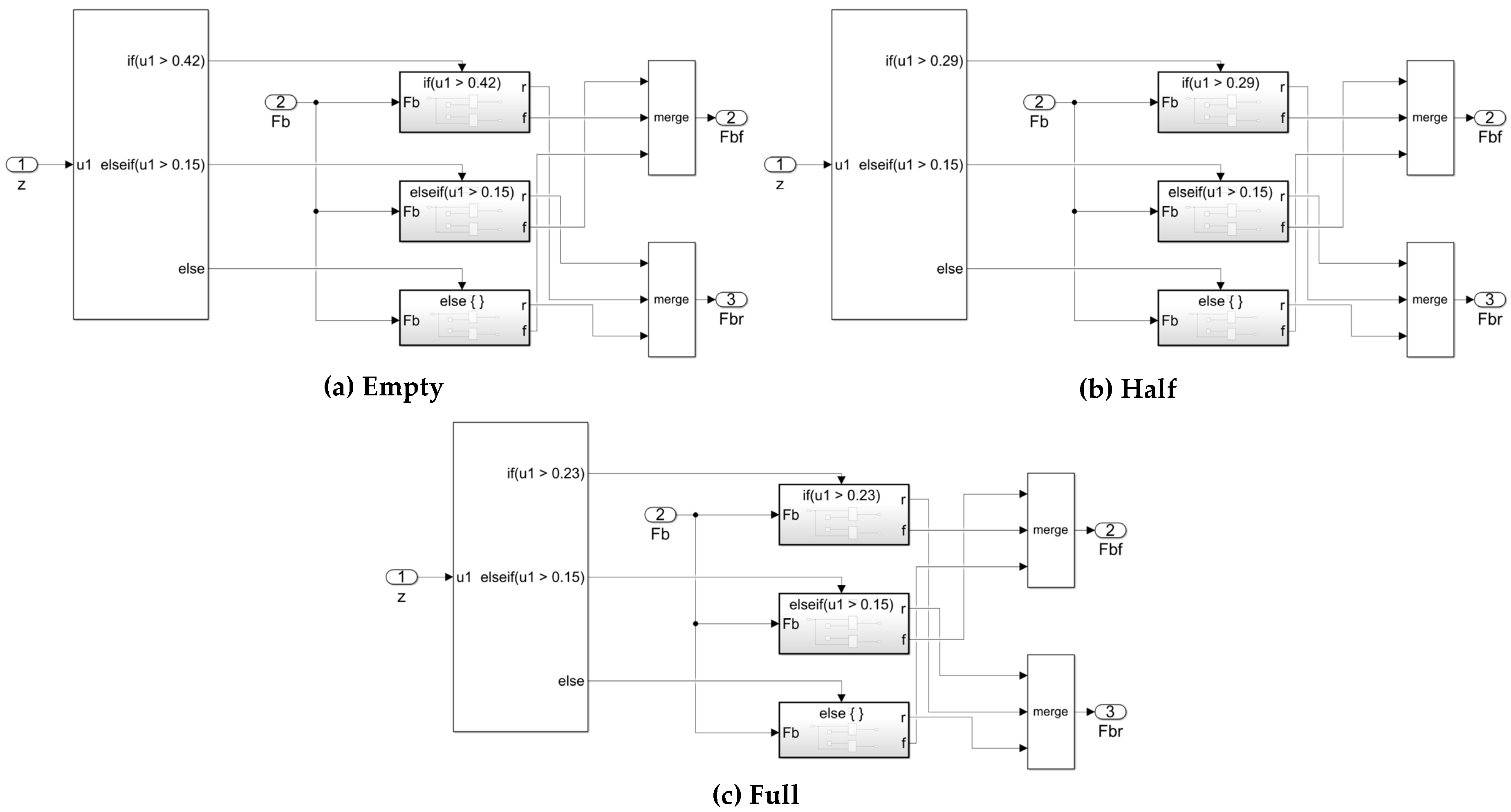
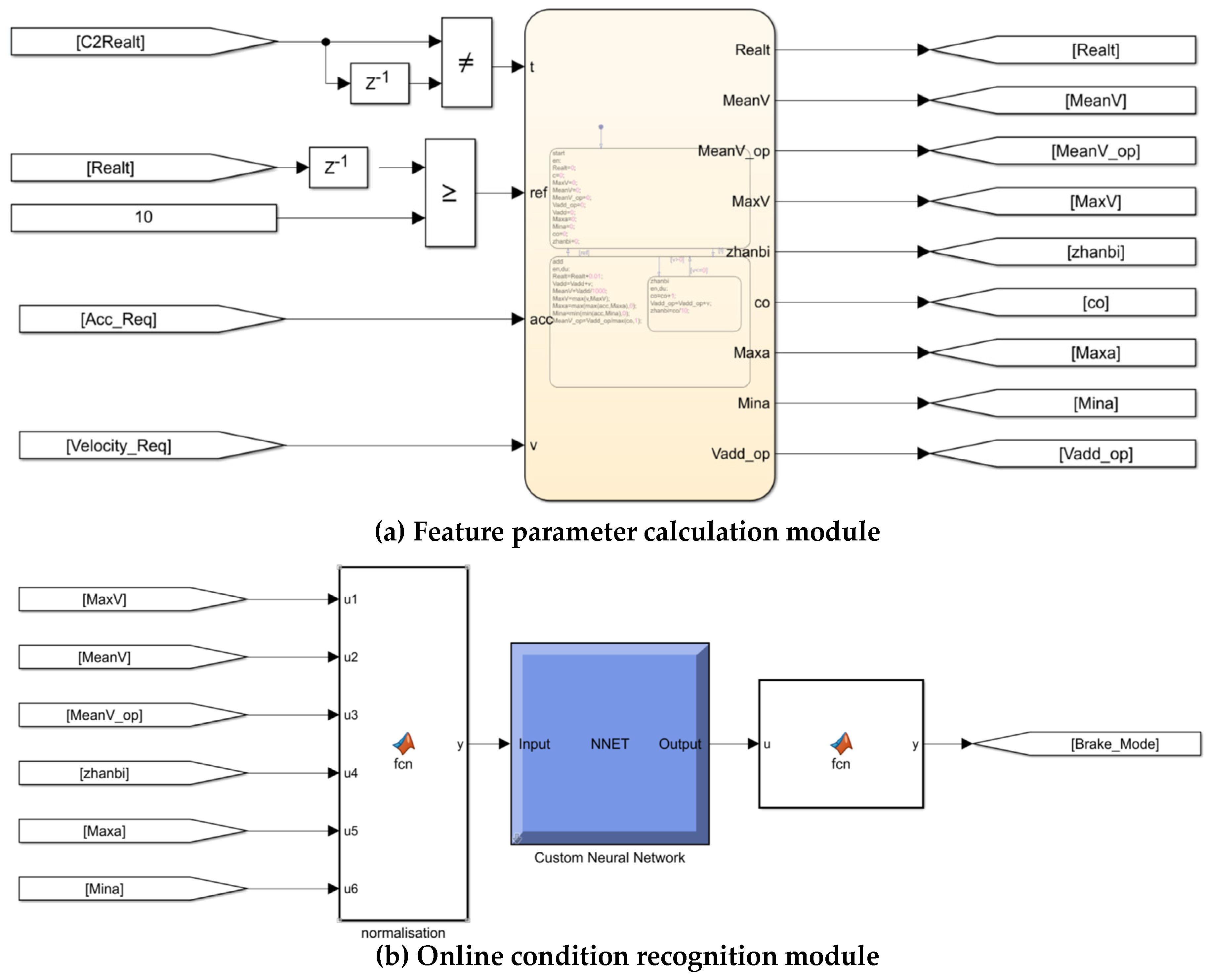
Simulink is a visual simulation tool in Matlab that is widely used in modelling and simulation applications for linear systems, nonlinear systems, digital control, and digital signal processing, and it can convert the constructed control model into a DLL file to perform data transfer and a joint simulation with AVL-Cruise software to improve research efficiency. Thus, based on the regenerative braking strategy designed in the previous chapters, in this study, the regenerative braking strategy model based on condition identification was built in Simulink, as shown in
Figure 14 and
Figure 15.
5. Simulation Analysis
The most commonly used verification method in the simulation process of energy management strategy construction is Matlab/Simulink 2022(a) and AVL-Cruise v.2019 joint simulation. To ensure the rigour of the simulation, the C-WTVC cycle, and a sampling synthesis of the cycle based on the clustering results of the previous paper, were selected. The joint simulation analysis was conducted using the Matlab DLL interface method to verify the design of this paper’s control strategy’s effectiveness. With reference to the duration of the international standard conditions, the duration of the synthetic cycle in this study was set to 1800 s, in which the duration of each type of conditions was determined according to the following formula:
where
is the duration of the i category of the synthetic conditions;
is the time occupied by the ith category of all kinematic segments;
is the duration of all kinematic segments; and
is the target duration of the synthetic conditions.
To ensure that the research was rigorous, a fixed-ratio strategy where and , and a fuzzy control strategy with the vehicle velocity, , and brake pedal opening as inputs, and the electromechanical brake force distribution as the output, were selected for comparison in the simulation process for the simulation analysis.
The braking energy recovery rate, i.e., the ratio of energy recovered to the energy consumed during braking, was used as an evaluation index for the simulation, as shown in Equation (28).
where
is the brake consumption energy recovery rate;
is the recovered energy (kJ); and
is the consumed energy (kJ).
5.1. Comparative Analysis of Simulation under C-WTVC Cycle
The simulation was carried out at room temperature (20 °C) with a road adhesion coefficient of 0.7 and windless environment. During the simulation, the COA-BPNN identified the characteristic information of the working conditions for 10 s of history, and since the first identification occurred in less than 10 s, the simulated velocity was set to 0 for the first 10 s.
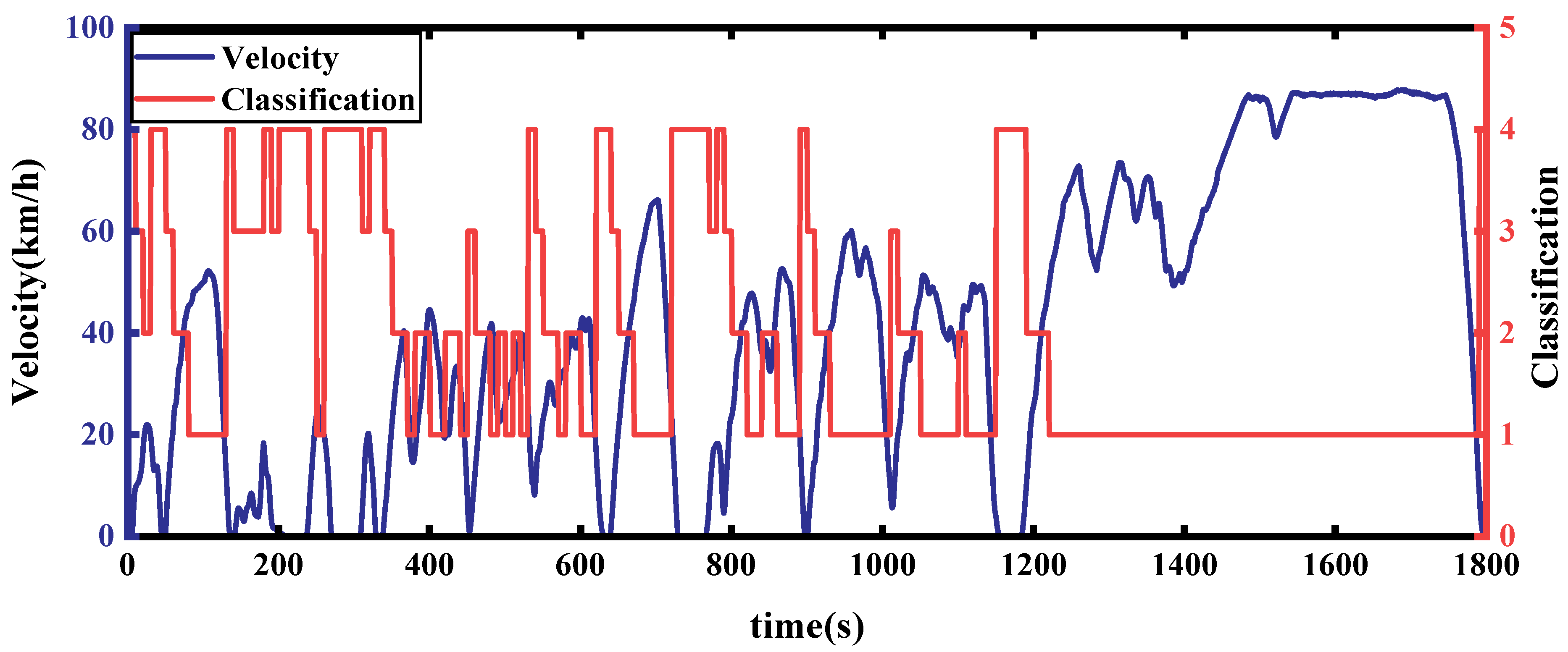
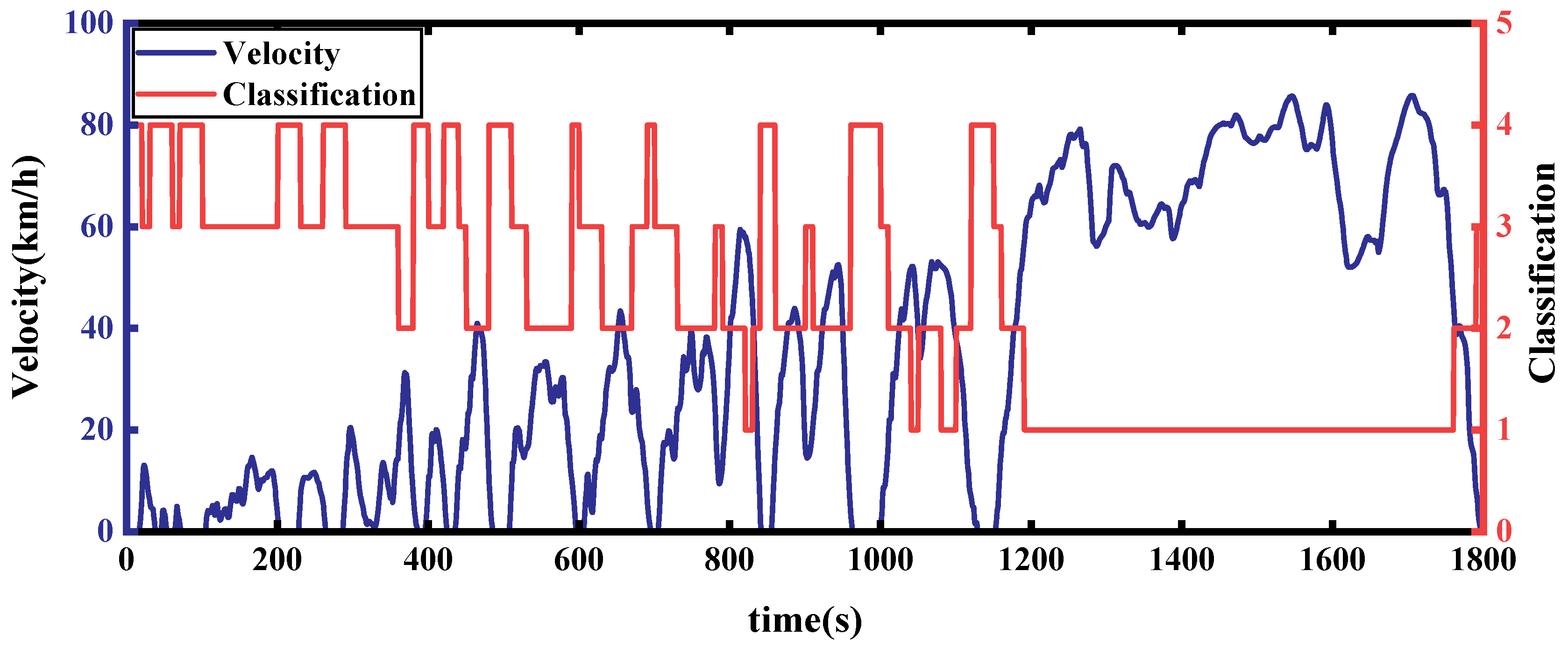
Figure 16 shows the results of the working condition identification for the C-WTVC; the red line is the category of a moment identified by the COA-BPNN, where 1, 2, 3, and 4 correspond to highway, suburban, urban smooth, and urban congestion conditions, respectively; the blue line is the vehicle velocity; and the accuracy of the identification results is 97.3%, indicating an almost perfectly accurate recognition.
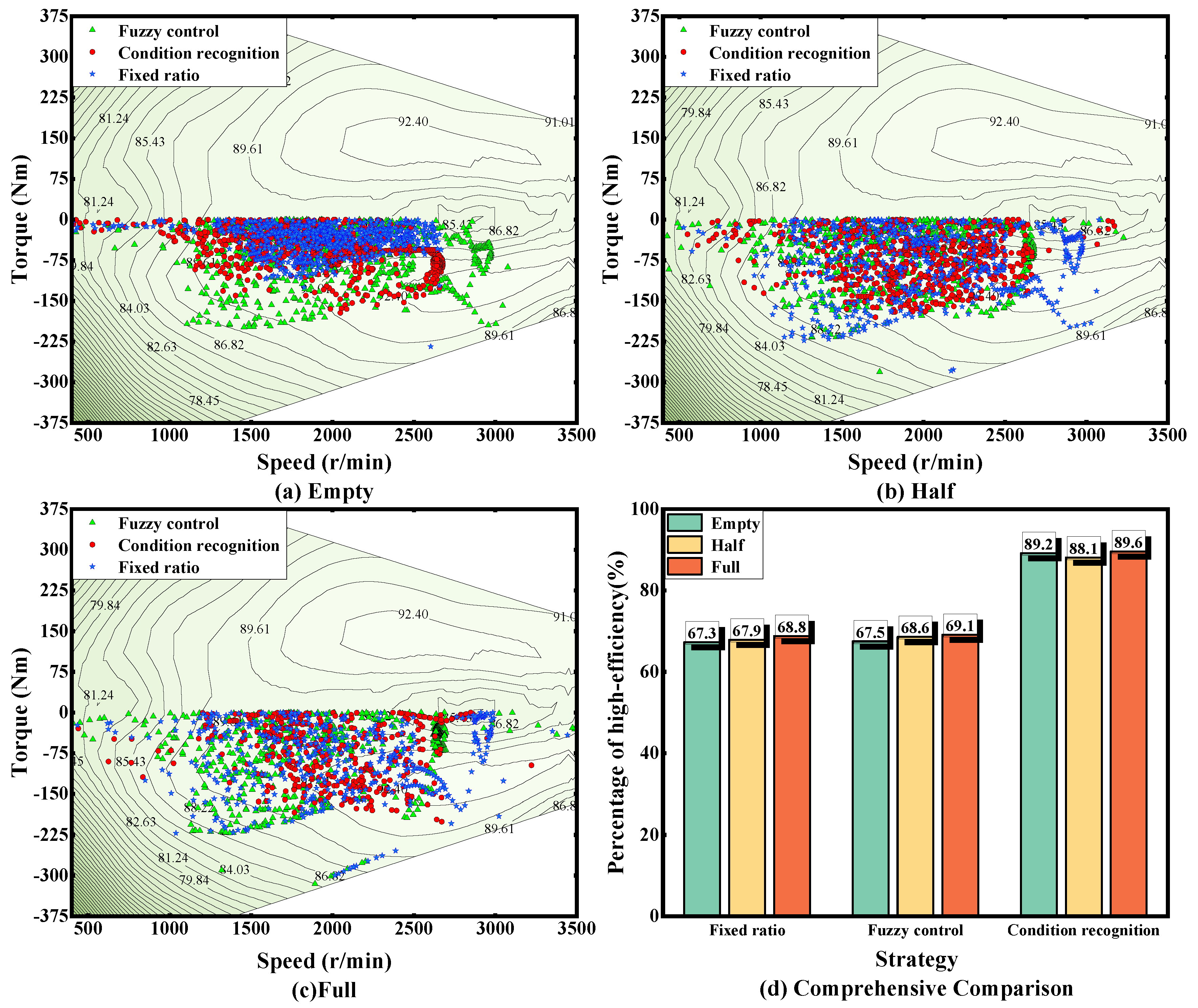
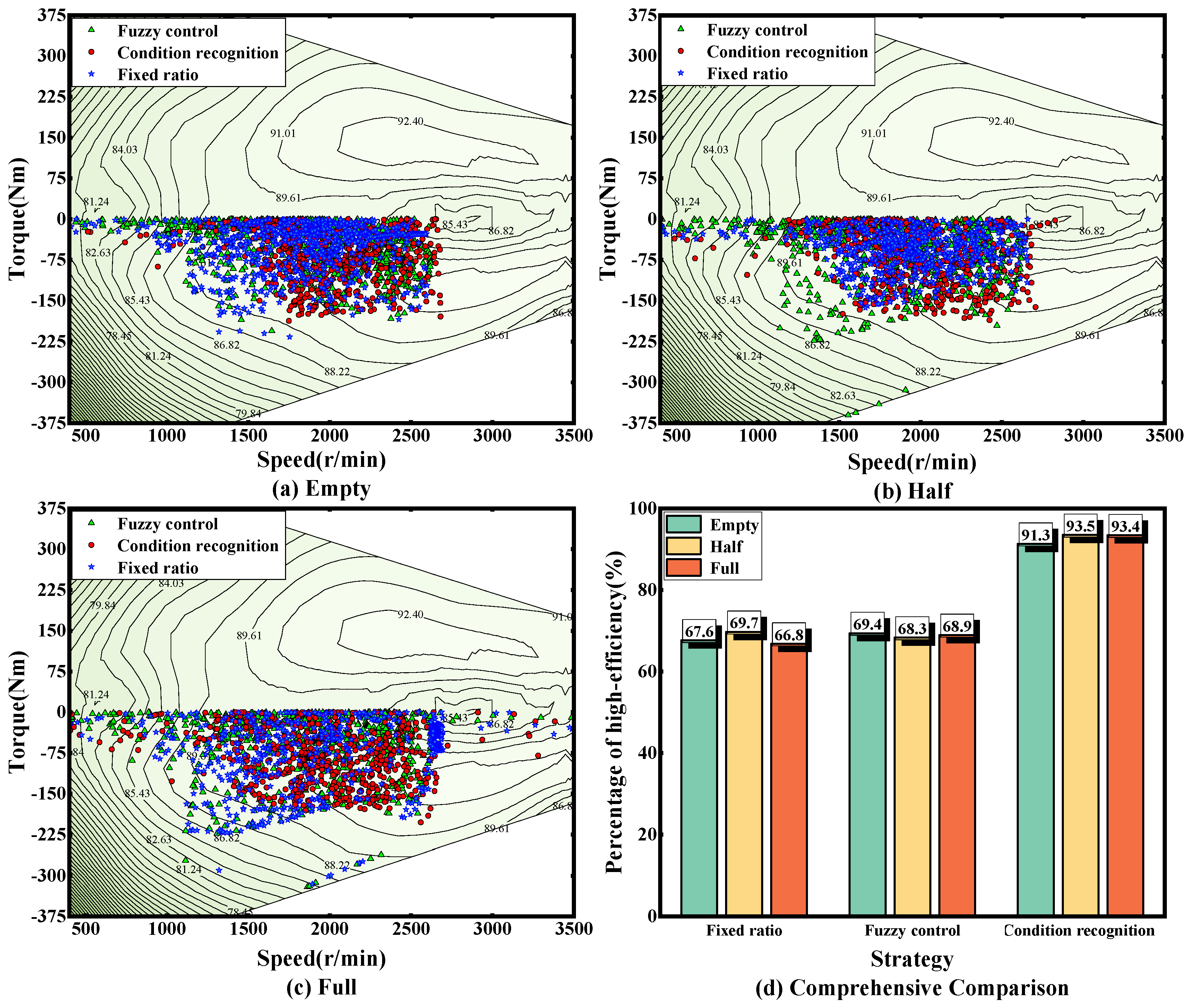
Figure 17 shows the electric motor working points during braking under three loads under C-WTVC conditions, from which it can be clearly seen that the regenerative braking strategy based on the condition identification in this paper is obviously more clustered in the medium- and high-efficiency range during braking, with fewer low-speed and low-torque working points. On the other hand, the electric motor working points are more scattered for the fuzzy control strategy and the fixed-ratio strategy. The period in which the electric motor efficiency is higher than the 89% contour is referred to as the high-efficiency interval. Within this interval, the proportions of the regenerative brake strategy based on condition detection under empty-, half- and full-load states are 89.2%, 88.1%, and 89.6%, respectively; for the fuzzy control strategy, the proportions are 67.5%, 68.6%, and 69.1%, respectively; and for the fixed-ratio strategy, they are 67.3%, 67.9%, and 68.8%, respectively. It can be seen that the regenerative braking strategy based on the identification of the working conditions can effectively limit the electric motor to work in the high-efficiency zone and increase the recovery efficiency.
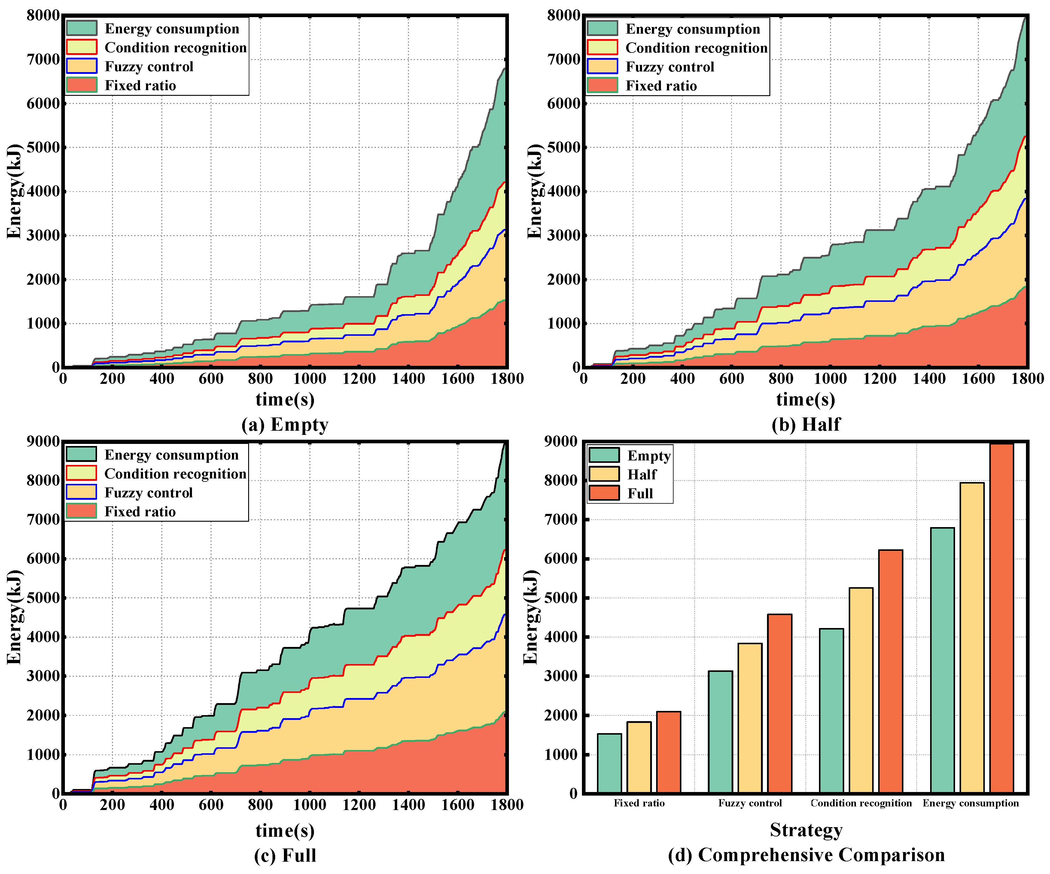
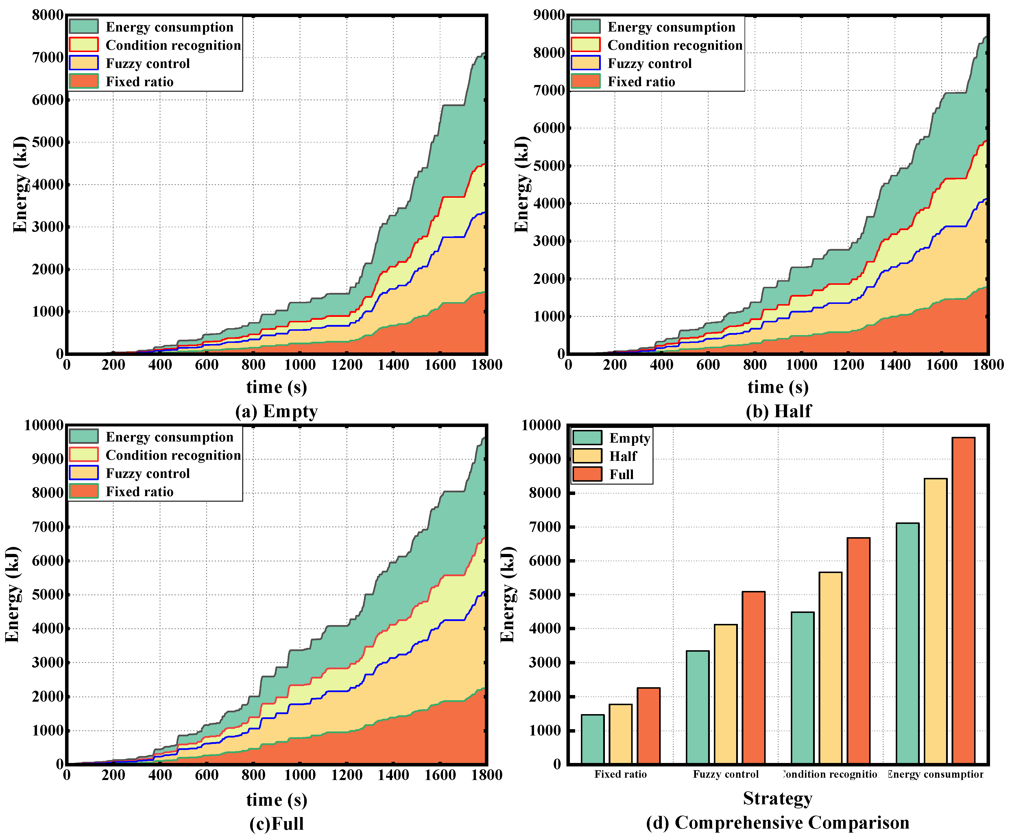
Figure 18 shows a comparison of the total energy consumed and energy recovered from braking for the three load states under the C-WTVC cycle, and it can be clearly seen that, as the load mass of the vehicle rises, the total energy generated during braking increases, and the energy recovered from regenerative braking thus also increases. It is also clear from the graph that the strategy outlined in this paper recovers more energy, regardless of the load.
Table 7 shows the simulation results for three kinds of loads under the C-WTVC cycle, from which it can be seen that under empty-, half- and full-load states, the energy recovery rate of this study’s strategy is improved by 34.6%, 36.9%, and 36%, respectively, compared to that observed with the fuzzy control strategy, and the energy recovery rate with the fixed-ratio strategy is improved by 175%, 186.3%, and 197.6%. This indicates that the regenerative braking strategy based on the identification of working conditions can effectively improve the energy recovery rate of the whole vehicle, by ensuring that the braking effect of the whole vehicle is used.
5.2. Comparative Analysis of Simulation under Synthetic Cycle
The synthetic cycle includes urban congestion, urban smooth, suburban, and highway conditions, with more aggressive driving behaviours, including higher rates of acceleration and deceleration. The entire cycle lasts for a total of 1800 s.
Figure 19 shows the working condition identification results for the synthetic working conditions in the simulation process, and the accuracy of the identification results is 98.76%.
Figure 20 shows the working points of the electric motor during braking under synthetic conditions, and it can be seen that, under synthetic conditions, the approximate distribution of the working points is consistent with that of the C-WTVC cycle, indicating that the strategy in this paper is highly adaptable to working conditions.
Figure 21 shows a comparison of the total energy consumed and energy recovered for braking in the three load states under a synthetic cycle, from which it is clear that the strategy of this paper recovers more energy at any load.
Table 8 shows the simulation results for the three loads under synthetic conditions, from which it can be seen that the energy recovery of the strategy in this study was improved by 34.2%, 37.4%, and 31.3% compared with that achieved with the fuzzy control strategy, and by 206.3%, 218.5%, and 197.2% compared with that observed with the fixed-ratio strategy, respectively, under empty, half, and full loads. It can be seen that the regenerative braking strategy based on condition identification resulted in a much higher braking energy recovery than the fuzzy control strategy and the fixed-ratio strategy in both the C-WTVC and synthetic cycles, showing the superiority of the strategy in this paper.


