Abstract
Air quality directly affects the health of humans. The health implications of poor air quality are recognized by professionals and the public alike and these concerns have driven both the proliferation of formal sensor networks, but also low-cost sensors which can be used in the home. The advancement of technology in recent years has also led to the rapid development of low-cost sensors. Given that citizens are concerned about the air quality of the environment in which they live, they are turning to the supply of low-cost sensors, as they are affordable. The question of the reliability of measurements from low-cost sensors remains an area of research. In this research work, the optimization of ozone (O3) and nitrogen dioxide (NO2) measurements of low-cost electrochemical air quality sensors is investigated by applying nonlinear regression, using a second-order polynomial equation as a correction factor. The proposed correction method is implementable in IoT devices, as it does not require high computational resources. The results show that the measurements are susceptible to correction, with the effect that the corrected values are close to the actual values obtained by the reference instruments of the Department of Environmental Pollution Control Project of Athens (PERPA), a service of the Greek Ministry of the Environment and Energy.
1. Introduction
Air quality is a vital factor for human health, particularly in densely populated areas. Low-cost sensors have emerged on the market in recent years as a consequence of the development of technology, presumably also because of demand or the growth of a market for small-scale measurements. Citizens are increasingly using these sensors to monitor the air quality in their area. Research centers and governmental agencies are engaged in monitoring air quality in all countries, using expensive scientific instruments to ensure the reliability of the measurements, resulting in only a few such systems covering large areas, like cities [1]. The use of low-cost sensors can help develop a large spatial network of measurements for a region [2]. Low-cost sensors can be used as a complement to monitor the air quality of a region and not as a replacement for expensive scientific equipment [3]. The reliability of low-cost sensor measurements is an ongoing area of research and study in the scientific community.
The following research papers present methodologies aiming at correcting and visualizing the measurements obtained from these sensors. Many manufacturers and research groups have devoted themselves to developing low-cost sensors and evaluating their performance in laboratory conditions [4,5,6,7]. Low-cost electrochemical air quality sensors use a specific measurement methodology [8,9,10]. All low-cost sensors exhibit errors, resulting in differences in measurement data compared to reference data. There are two main sources of error in measurements from low-cost sensors [11], the internal errors, which are based on the operating principle of the sensor, including dynamic detection limits, nonlinear sensor response and displacement, and the external errors, which occur according to the working conditions, with the main one the low selectivity of the target gas, affected by cross-sensitivity with other gases. These errors can be reduced using laboratory and simplified calibration methods.
Therefore, many investigations into low-cost sensors have demonstrated the development of sensor calibration in the field [12]. These include low-cost sensor calibration of carbon monoxide (CO) [13,14], nitrogen dioxide (NO2) [13,14,15], sulfur dioxide (SO2) [13,14], ozone (O3) [13,15], and particulate matter (PM) [16,17,18]. In [19] the evaluation of the performance of low-cost particle sensors indicated the ability of the sensors to monitor particle concentrations with relatively high linearity and moderate repeatability. In another work [20], the effect of relative humidity (RH) and gas sample flow rate on sensor calibration and sensitivity was investigated.
The performance of the low-cost sensors was evaluated in the field, in an ambient atmosphere. Many of the aforementioned studies focused on the influence of meteorological factors, such as temperature (T), RH, wind, sunlight, etc., and proposed calibration schemes based on long-term evaluation in urban or suburban environments [21,22,23,24]. In addition, other studies have reported on the effect of cross-sensitivity in low-cost sensors [25,26,27]. Many methods have been used by research groups to calibrate air quality sensors, such as linear regression (LR), multiple linear regression (MLR), random forest (RF), artificial neural network (ANN), support vector machine (SVM), and support vector regression (SVR) [28]. The LR and MLR methods are commonly for calibration of low-cost sensor data, and symmetric variables are used to improve the calibrations. However, LR shows a lower R2 correlation score and should be avoided for gas sensors [29,30]. RF, ANN, SVM, and SVR are supervised learning technique methods and show significant improvement in the R2 correlation coefficient in most sensors. However, their application requires a large amount of data for training each model [31,32]. The simplest correction methods are presented by the Kalman filtering [33] and LASSO regression [34] approaches, as well as the measurements variation limits [35] approach. According to manufacturers, the lifetime of low-cost electrochemical sensors is set at 1 to 2 years, and during its operation the change in sensor response is referred to as aging [36,37]. Specifically, [37] reports on the identification of aging factors in low-cost electrochemical sensors for measurement corrections. Other research works present the application of low-cost sensors for air quality monitoring [38,39,40], and [41] presents the artificial intelligence method of a memory-based precise calibration of a cost-efficient NO2 sensor, and data reliability and fault diagnostics for an air quality monitoring station based on low-cost sensors and active redundancy, studied in [42].
As a statistical model, nonlinear regression is the application of regression analysis, where observational data are captured by a function that includes a nonlinear combination of the model parameters and depends on one or more independent variables. The data are tabulated and adjusted accordingly using a method of successive approximations. In general, linear regression shows the correlation between two variables using a straight line, while nonlinear regression shows the correlation between variables using a curve. The authors of [43] show the results of nonlinear regression on low-cost microparticle data from sensors. By applying probabilistic gradient boosted decision trees (GBDTs), direct field calibration of raw PM2.5 sensor data is achieved. The use of probabilistic GBDTs improves point accuracies and distribution compared to the linear model. In [44] the application of calibration models using nonlinear machine learning boosting algorithms, namely Stochastic Gradient Boosting Regressor, yielded better results than those obtained using artificial neural networks and linear regression approaches.
In this research work, the degree of correction in low-cost sensor measurements is investigated by applying nonlinear regression to data obtained by low-cost electrochemical pollutant gas sensor measurement, aiming to identify a polynomial function that serves as a correction factor in low-cost sensor measurements, with the final result being the optimization of these measurements. In addition, the methodologies of time scaling and seasonality scale are investigated to evaluate the results using the nonlinear regression approach. The choice of a polynomial function as a correction tool finds immediate application for integration in IoT devices, as it does not require computational resources, unlike other techniques, such as artificial neural networks, etc. The article is structured as follows: Section 2 presents the Materials and Methods, Section 3 discusses the Results, Section 4 covers the Discussion and Section 5 covers the Conclusions.
2. Materials and Methods
2.1. Instrumentation
Three low-cost air quality monitoring stations [15] with unique identifiers (N1, N2, N3) were used to conduct this experiment. The design and implementation of the low-cost gas quality monitoring stations were carried out by the Electronic Devices and Materials Research Laboratory (EDML) of the Department of Electrical and Electronics Engineering of the University of West Attica in Greece. Details of the monitoring stations’ design and implementation can be found in previous works [15,35]. The stations were installed at the same place, near to official instrumentation from the Ministry of Environment and Energy of Greece (PERPA) [45] at a height of 6–8 m. The monitoring stations were installed in Athens city center and installation details regarding the locations, the sampling rate and the official instrumentation used for the on-site measurements are presented in [33]. The two locations are close to each other and show the same air quality conditions. Commercial scientific instruments for monitoring air quality have been installed at the Environmental Pollution Control Project of Athens (PERPA) facilities in the center of Athens. Specifically, the installed devices for measuring air pollutants are the HORIBA APOA-360 for ozone and the HORIBA APNA-360 for nitrogen dioxide. Pollutants are measured continuously throughout the 24-h period. The response time of the automatic analyzers is one minute, while the hourly average pollution values are calculated hourly. The methods of measurement of air pollutants are carried out for nitrogen dioxide by chemiluminescent science and for ozone by ultraviolet absorption. As for the automatic analyzers, field calibration is carried out by dynamic dilution every month and after each repair. The details that refer to the used NO2 and O3 electrochemical sensors (manufacturer AlphaSense (Essex, UK) and models: NO2–NO2-B43F [46] and O3–OX-B431 [47]) as well as the initial calibration of the sensors are presented in previous works [34]. The time period of the measurements and evaluation was 14 April 2021 to 13 May 2021.
2.2. Data Elaboration
Nonlinear regression is a type of regression where, during analysis, observational data are modelled according to a function that is a nonlinear combination of the model parameters and depends on one or more independent variables. The data are fitted by a method of successive approximations. The use of nonlinear regression may be made as not all phenomena are described by linear models, as well as for cases of data where linear regression is less accurate than nonlinear regression. In general, a function is nonlinear with respect to its constituent parameters. For the purposes of this work a polynomial equation of second degree was chosen. Polynomials offer a broader scope for representing functions and relationships between variables than linear equations, enabling more complex modeling and flexible curve fitting, and enhancing predictive accuracy. A second-degree polynomial equation is expressed in Equation (1).
where is the independent variable, and , , , are the coefficients.
Nonlinear functions that can be used include logarithmic functions, exponential functions, trigonometric functions, etc.
To ensure thorough analysis of the results, experiments were conducted on a weekly and monthly basis. Polynomial functions were identified weekly for each sensor and gas and the monthly function was derived from monthly data and refined by incorporating weekly polynomial functions. In addition, a comprehensive study was conducted on time scaling and seasonality correction using the nonlinear regression approach.
The methodology for applying nonlinear regression to low-cost electrochemical sensor data is described in four steps:
- Hourly measurements of low-cost sensors of the same type were averaged.
- The averaged values were correlated with the reference values and the degree of correlation was expressed by a second-order polynomial function.
In the same way, the hourly measurements of each sensor were correlated with the reference measurements and the degree of correlation was expressed by a second-degree polynomial function.
For the purpose of evaluating the results, this procedure was carried out on a weekly basis for one month’s measurements.
- 3.
- From the monthly polynomial correlations, the coefficients of the polynomial correction function were estimated.
- 4.
- The monthly polynomial correction function was applied to the low-cost sensor measurements and the results were re-evaluated.
Finally, the Root Mean Square Error (RMSE), Mean Absolute Deviation (MAD), and Mean Absolute Error (MAE) methods were used to evaluate the nonlinear method results, both for weekly and monthly data.
The measurements analyzed below relate to gaseous pollutants, such as nitrogen dioxide and ozone. The data from both the low-cost and reference gas sensors have been taken on an hourly basis. Simple nonlinear regression is applied to the data to identify a polynomial function that can be used as a correction factor for the data from the low-cost sensors. The measurements (primary and corrected by nonlinear regression (NLR)) analyzed below relate to gaseous pollutants, such as nitrogen dioxide and ozone. The data from both the low-cost (Ν1, Ν2, Ν3) and reference gas sensors have been taken on an hourly basis. Simple nonlinear regression is applied to the data to identify a polynomial function that can be used as a correction factor for the data from the low-cost sensors.
For the needs of the experiment, one month’s data (14 April 2021 to 13 May 2021) are studied, since according to [37], the ageing of the sensors has an effect on the measurements. To establish a more generalized study, nonlinear regression is applied on a daily basis, weekly basis, and monthly basis, for both types of sensors.
A series of replicated experiments were performed to determine the degree of the polynomial function. The results showed that a polynomial function of 2nd degree is sufficient to give satisfactory results in terms of the degree of correlation. The polynomial function of a higher degree, especially on one month’s data, shows a further improvement of up to 1% in relation to the polynomial function of 2nd degree.
3. Results
The results of nonlinear regression as a correction factor in ozone (O3) and nitrogen dioxide (NO2) concentration measurements are presented here.
Given that low-cost electrochemical gas quality sensors consisting of four electrodes (working electrode, auxiliary electrode, counter electrode, and reference electrode) were used, the procedure during the initial calibration and normalization of the primary measurements is then presented [34]. The first step is to correct the working electrode value according to manufacturer by the specific properties of each sensor (electronic zero value) and the temperature coefficient. An Individual Sensor Board (ISB) circuit, as reported by Alphasense, provides both working electrode and auxiliary electrode measurements in mV. The conversion of the working and auxiliary electrode voltages to target gas concentration is suggested by Alphasense’s Equation (2) [48], which includes the ambient temperature
where represents the corrected value of the working electrode, represents the measured value of the working electrode, represents the measured value of the auxiliary electrode, represents the ambient temperature coefficient, represents the electronic zero value of the working electrode, and represents the electronic zero value of the auxiliary electrode. The values of and are given by the manufacturer for each sensor. The second step is to calculate the concentration (ppb) of gas pollutant. The concentration measurement is given by dividing the corrected output voltage , by , as shown in Equation (3), the sensor sensitivity is also given for each sensor by the manufacturer
where is the concentration measurement of the gas pollutant, is the corrected working electrode value of the target gas given by Equation (2), and is given by the sensor manufacturer.
The third step is to calculate a calibration function. According to the manufacturer, a function must be applied when calibrating the sensors so that the corrected values of the measurements with this function are close to the reference values. Two correction factors [15] are calculated during the calibration period when co-locating the low-cost monitoring station close to official instruments. The formula that yields the final corrected values by combining the two correction factors and the sensor measurements is shown in Equation (4)
where is the calibrated gas sensor value, is the corrected measurement concentration value of the gas pollutant by Equation (3), where A represents the level factor, which increases or decreases the measurement values to be corrected, and B represents the scaling factor, from which the corrected values of measurement are derived. The last step of the procedure is the conversion of ppb to μg/m3. The initial calibration period was carried out in February 2021, in the field, by co-installing low-cost sensors next to a reference instrument. This process resulted in the determination of the A and B coefficients for each low-cost gas sensor.
According to the manufacturer, to avoid incorrect gas measurements due to the cross-sensitivity of the Alphasense OX-B431 sensor, Equation (5) must be applied to the measurements in order to obtain the O3 and NO2 concentrations, since the O3 electrochemical sensors are also triggered by NO2,
where is the ozone concentration measurement, is the NO2 concentration value measured by the nitrogen dioxide sensor and is the concentration value measured by the ozone sensor.
3.1. O3 Weekly and Monthly Study
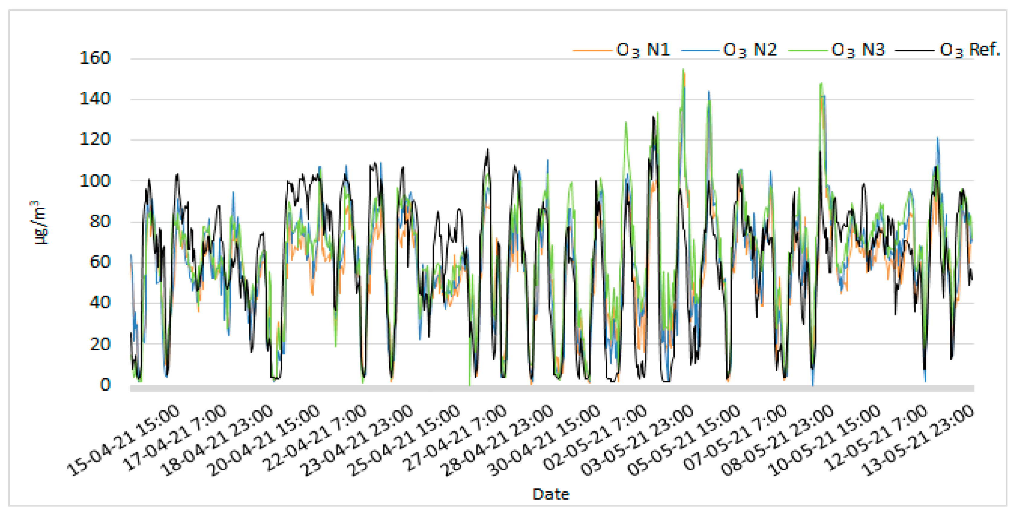
The obtained ozone concentration primary measurements, after the application of the correction equations, for all three low-cost ozone electrochemical sensors, relative to the reference measurements (PERPA), are shown in Figure 1.

Figure 1.
Time-series of O3 primary concentration measurements of low-cost monitoring stations and reference instruments.
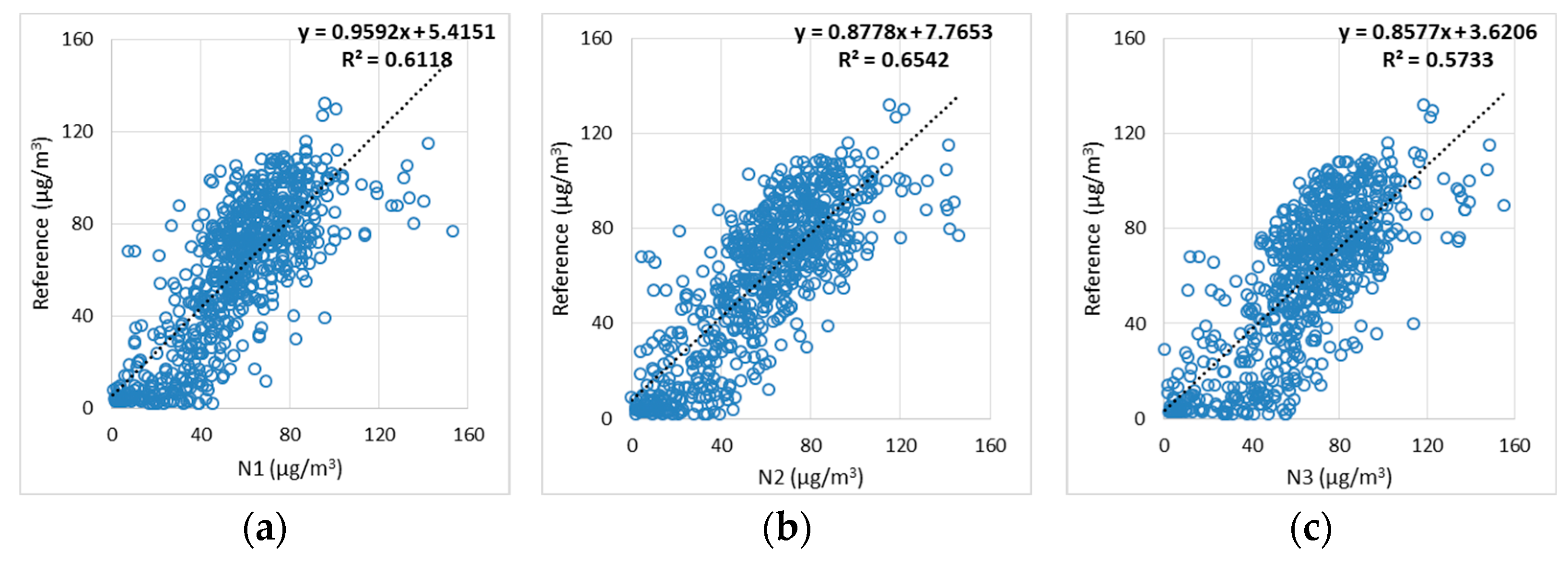
Figure 2 shows the scatterplots between the primary measurements of each ozone low-cost sensor and reference. The corresponding degree of correlation between the reference measurements and the primary measurements of the low-cost sensors is also presented.
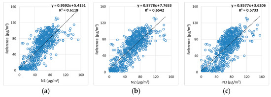
Figure 2.
Scatterplots of O3 primary measurements of N1, N2, N3 and reference measurements, (a) Scatterplot of O3 primary measurements of N1 and reference measurements, (b) Scatterplot of O3 primary measurements of N2 and reference measurements, (c) Scatterplot of O3 primary measurements of N3 and reference measurements.
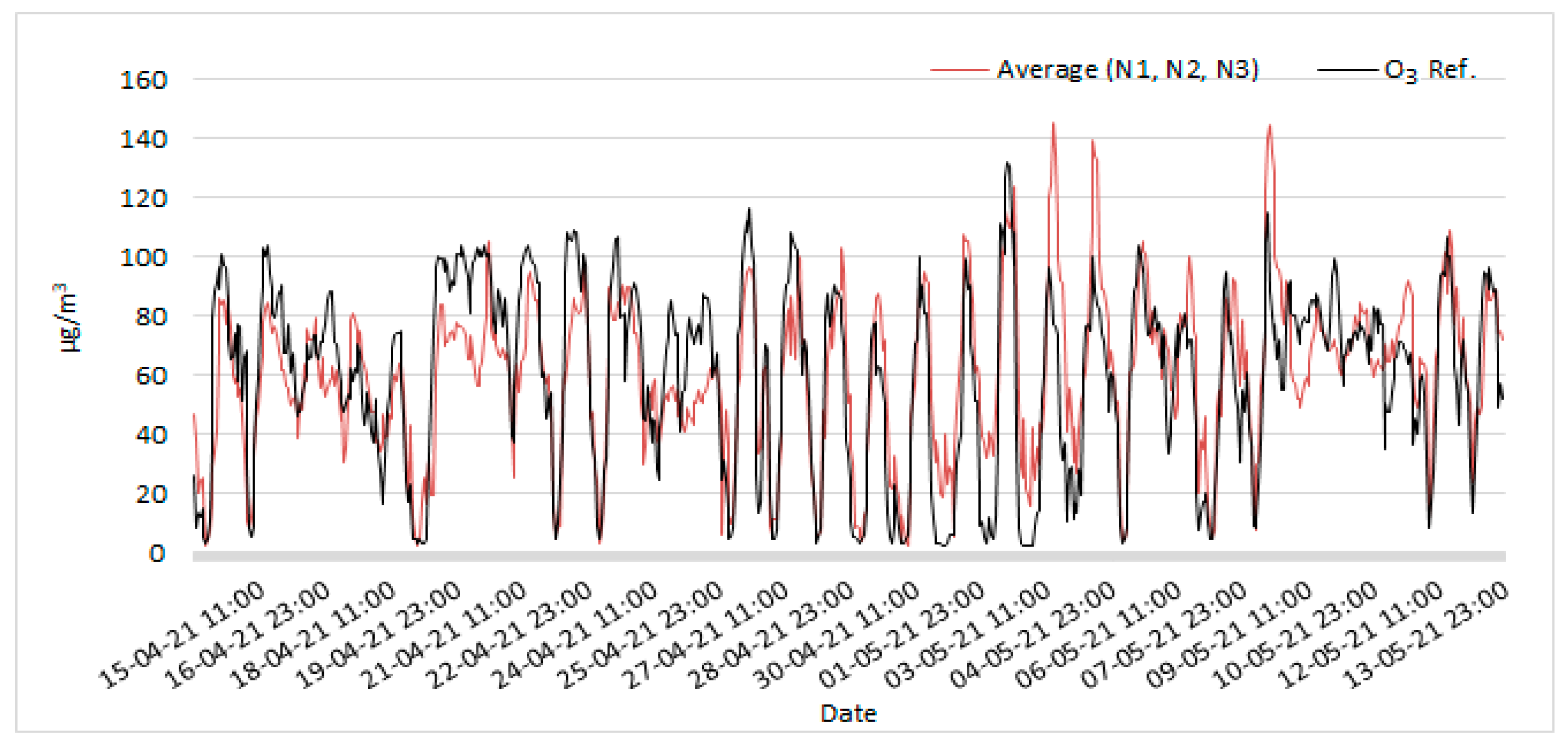
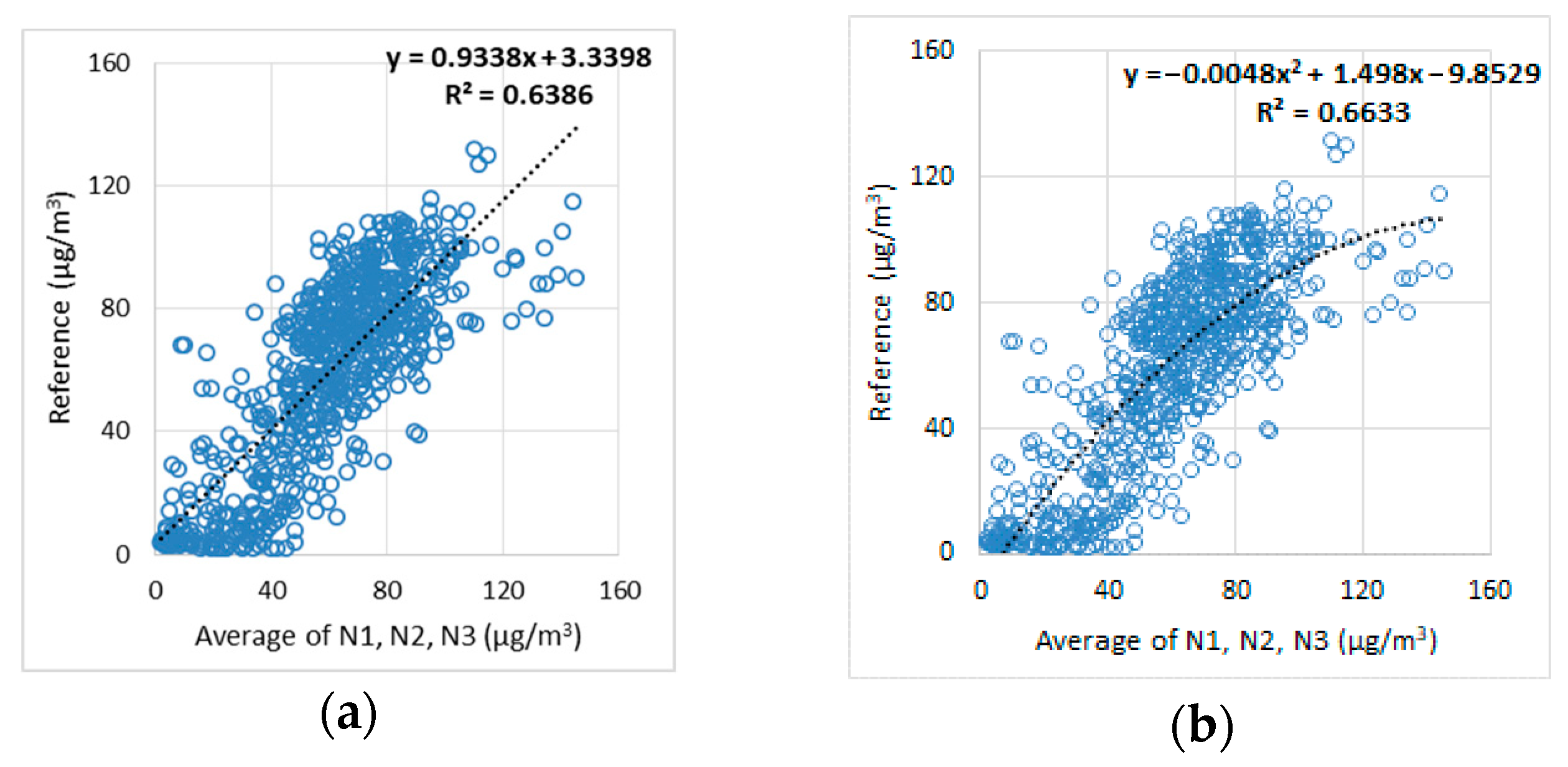
Figure 3 shows the average of the hourly ozone primary concentration measurements of the three low-cost sensors in relation to the reference measurements. Figure 4 shows both the simple linear regression scatter plot with the correlation coefficient and the nonlinear regression scatter plot with the polynomial equation of the correlation and the correlation degree of the ozone concentration measurements. Simple linear regression was used to show the dispersion and degree of correlation between the primary O3 concentration measurements from the low-cost sensors and the reference measurements.

Figure 3.
Time-series of the average of primary O3 concentration measurements of the three nodes (N1, N2, N3) low-cost monitoring stations and reference instruments.
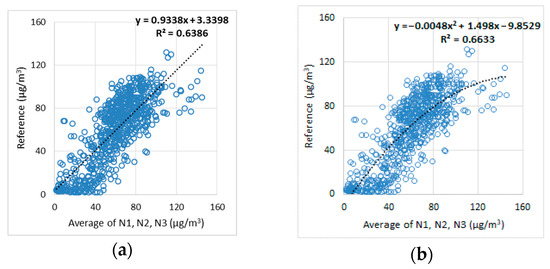
Figure 4.
Scatterplots of O3 primary measurements. (a) Scatterplot of O3 primary measurements of linear regression (LR) of average measurements (N1, N2, N3), (b) Scatterplot of O3 primary measurements of nonlinear (NLR), (polynomial function 2nd degree) regression of average measurements (N1, N2, N3).
In order to evaluate the proposed methodology, the NLR was applied for each week of the selected period and the extracted coefficients were compared. This was conducted to ensure the time stability of the NLR methodology. To investigate the behavior and variability of the coefficients of the linearity and the error, the application of the rolling regression took place for four weeks data on an hourly basis. Conclusively, to estimate the polynomial function, the experiment was performed on a weekly basis. From the data for each week, both a polynomial function and the degree of correlation of the data emerged.
The parameters of the rolling calibration, such as Alpha and Beta coefficients, Error, Correlation, and degree of correlation, are shown for the ozone concentrations, for the mean value of the primary data of the three ozone sensors with the reference data in Table 1, and for the mean value of the corrected data of the three ozone sensors with the reference data in Table 2.

Table 1.
Parameters of rolling regression between primary and reference measurements of O3 for four weeks.
Table 2.
Parameters of rolling regression between corrected and reference measurements of O3 for four weeks.
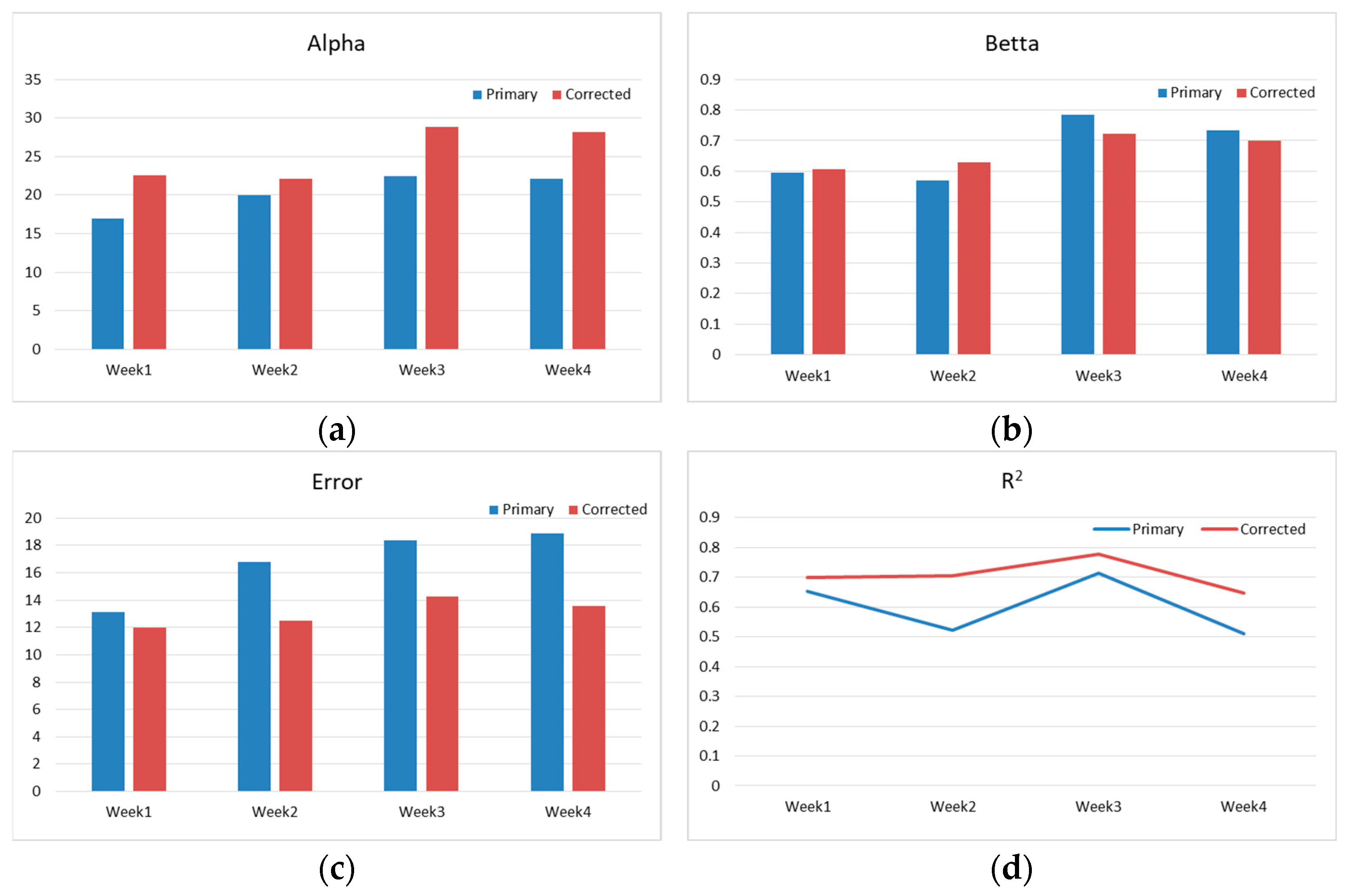
Figure 5 shows the coefficients (Alpha, Beta, Error, R2) both of the rolling regression of the average of the primary measurements of three ozone sensors and the reference, and the coefficients of the rolling regression of the average of the corrected by nonlinear regression measurements of three ozone sensors and the reference.

Figure 5.
Rolling regression coefficients of average of primary and average of corrected measurements (4 weeks) in respect to reference measurements of O3, (a) Alpha coefficient of average of primary and average of corrected measurements (4 weeks) in respect to reference measurements, (b) Beta coefficient of average of primary and average of corrected measurements (4 weeks) in respect to reference measurements, (c) Error of average of primary and average of corrected measurements (4 weeks) in respect to reference measurements, (d) Correlation degree (R2) coefficient of average of primary and average of corrected measurements (4 weeks) in respect to reference measurements.
Τhe observations extracted from Figure 5 in relation to the corrected data, in terms of the coefficients of the rolling regression for a four-week period for ozone, show an increase in the Alpha coefficient, while the Beta coefficient shows a slight shift, the Error shows an average improvement of 30%, and the correlation coefficient (R2) shows an improvement.
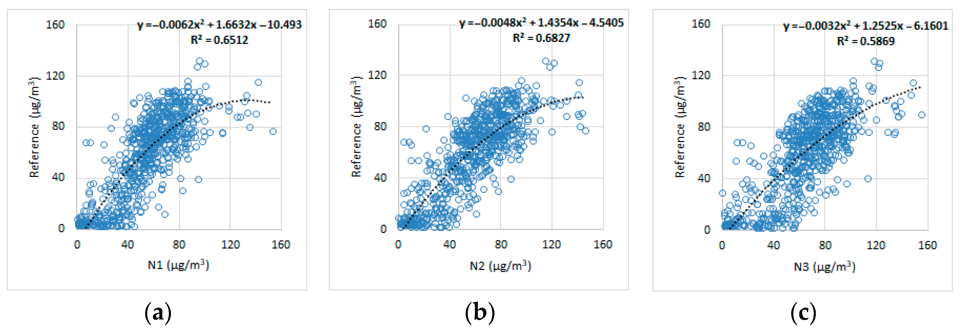
The expression of the nonlinear regression of the primary measurements of each low-cost O3 sensor in respect to the reference measurements is shown in Figure 6.
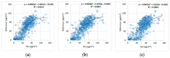
Figure 6.
Scatterplot of all O3 primary measurements in respect to the reference measurements of nonlinear (NLR), (polynomial function 2nd degree) regression. (a) Scatterplot between primary of N1 and reference measurements of O3 of nonlinear (NLR) regression, (b) Scatterplot between primary of N2 and reference measurements O3 of nonlinear (NLR) regression, (c) Scatterplot between primary of N3 and reference measurements O3 of nonlinear (NLR) regression.
The extraction of the coefficients of the nonlinear correction function for ozone (O3) was carried out as follows. From Figure 6 the square root of the average of the coefficients () of of N1, N2, N3, determines the value of the coefficient () of in the nonlinear correction equation. The value of the coefficient () of of the nonlinear correction equation can range from the maximum value that each coefficient () of shows in the scatter plots of the Figure 6 to their average value; the most appropriate value () of was chosen which gives the optimum effect on all sensors. The coefficient () of the nonlinear correction equation is obtained by taking the square root of the average of the coefficients () shown in the scatter plots of Figure 6.
According to the above data and the correlations of measurements, as shown in Figure 5 and Figure 6, the calculation of the polynomial function for the correction at the monthly level was carried out by the correctness, evaluation, and reliability of the results in respect to the reference data. The polynomial function acting on the sensor data as a correction factor to the ozone gas pollutant concentration measurements of low-cost sensors is described in Equation (6).
where , is the corrected concentration measurement of ozone and the is the primary concentration measurement of the ozone low-cost sensor.
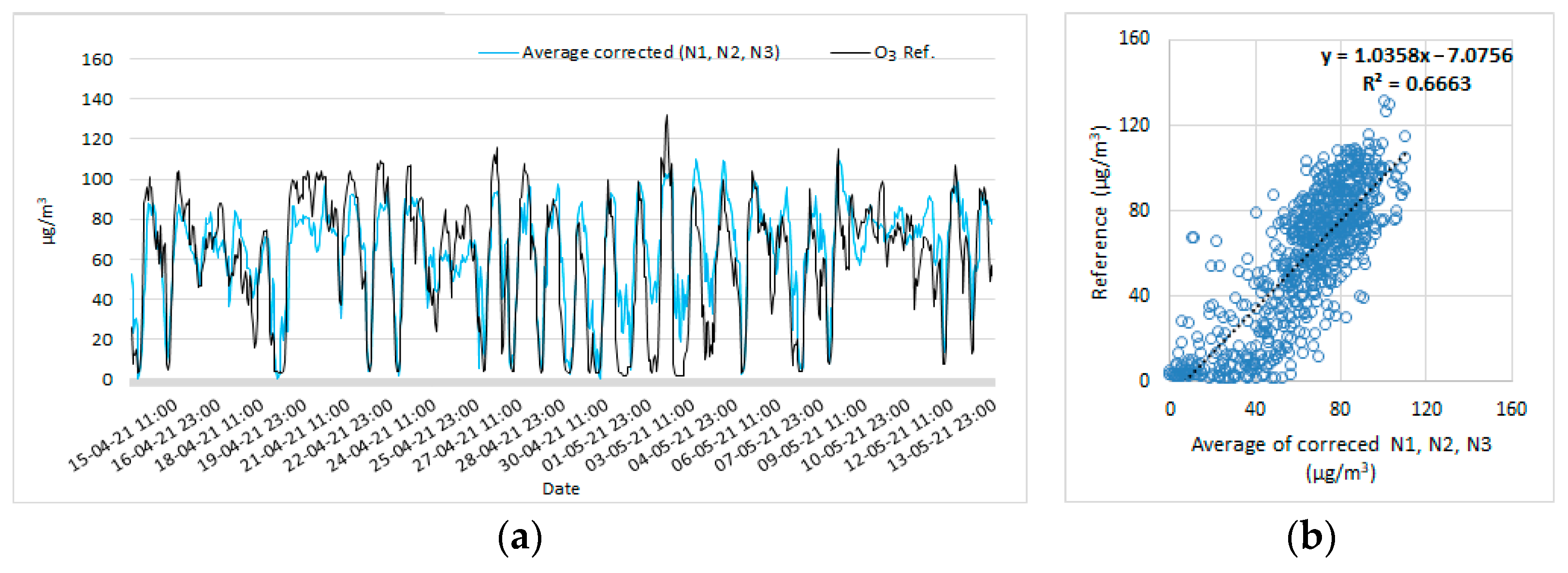
The polynomial function of Equation (6) was applied to the primary data of each low-cost ozone (O3) sensor. Figure 7 shows the time series and scatter plot of the average of corrected measurements in respects to reference measurements. The scatter plots of corrected measurements in comparison with reference measurements for ozone concentrations, are shown in Figure 8 for nodes N1, N2, N3, respectively.
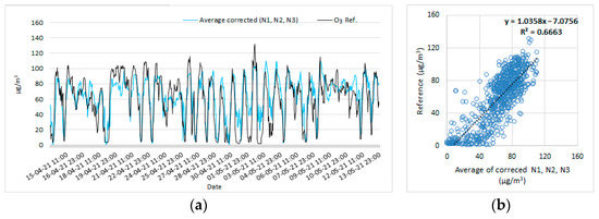
Figure 7.
Time-series and scatterplot of average of corrected O3 measurements of N1, N2, N3, and reference measurements, (a) Time-series of average of corrected O3 measurements of N1, N2, N3, and reference measurements, (b) Scatterplot of average of corrected O3 measurements of N1, N2, N3, and reference measurements.
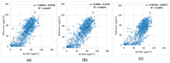
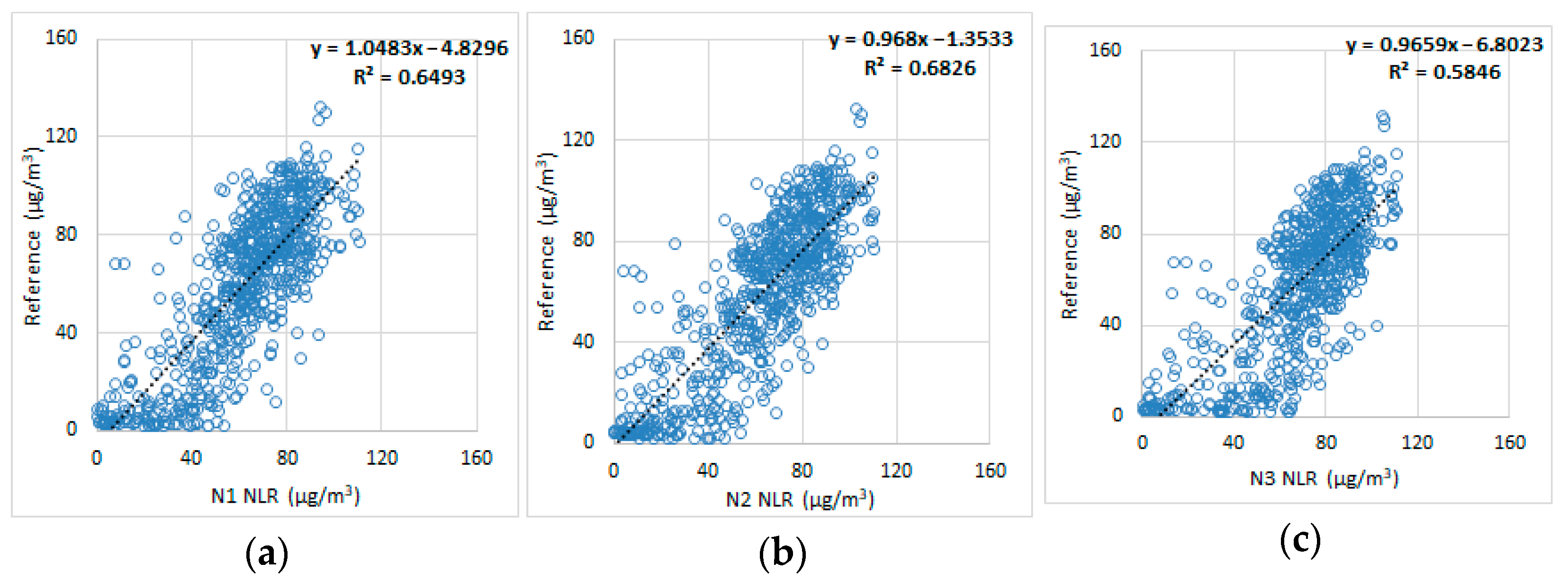
Figure 8.
Scatterplots of O3 corrected measurements of N1, N2, N3 and reference measurements, (a) Scatterplot of O3 corrected measurements of N1 and reference measurements, (b) Scatterplot of O3 corrected measurements of N2 and reference measurements, (c) Scatterplot of O3 corrected measurements of N3 and reference measurements.
3.2. NO2 Weekly and Monthly Study
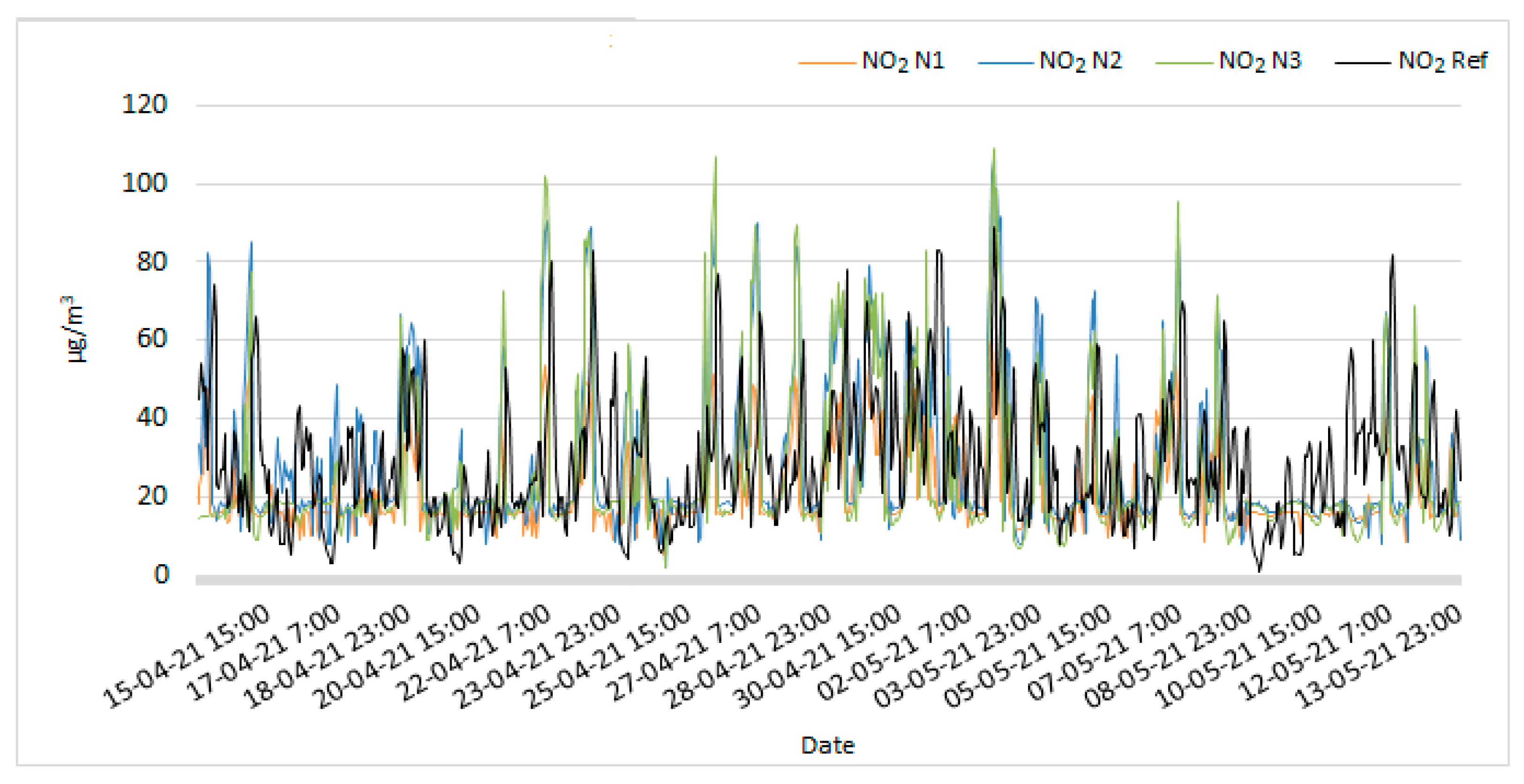
The obtained nitrogen dioxide concentration primary measurements, after application of the correction equations, for all three low-cost nitrogen dioxide electrochemical sensors, relative to the reference measurements, are shown in Figure 9.
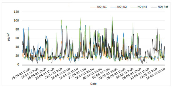
Figure 9.
Time-series of primary NO2 concentration measurements of low-cost monitoring stations and reference instruments.
Figure 10 shows the scatterplots between the measurements of each nitrogen dioxide low-cost sensor and reference. The corresponding degree of correlation between the reference measurements and the measurements of the low-cost sensors is also presented.
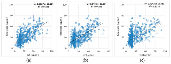
Figure 10.
Scatterplots of NO2 primary measurements of N1, N2, N3 and reference measurements, (a) Scatterplot of NO2 primary measurements of N1 and reference measurements, (b) Scatterplot of NO2 primary measurements of N3 and reference measurements, (c) Scatterplot of NO2 primary measurements of N3 and reference measurements.
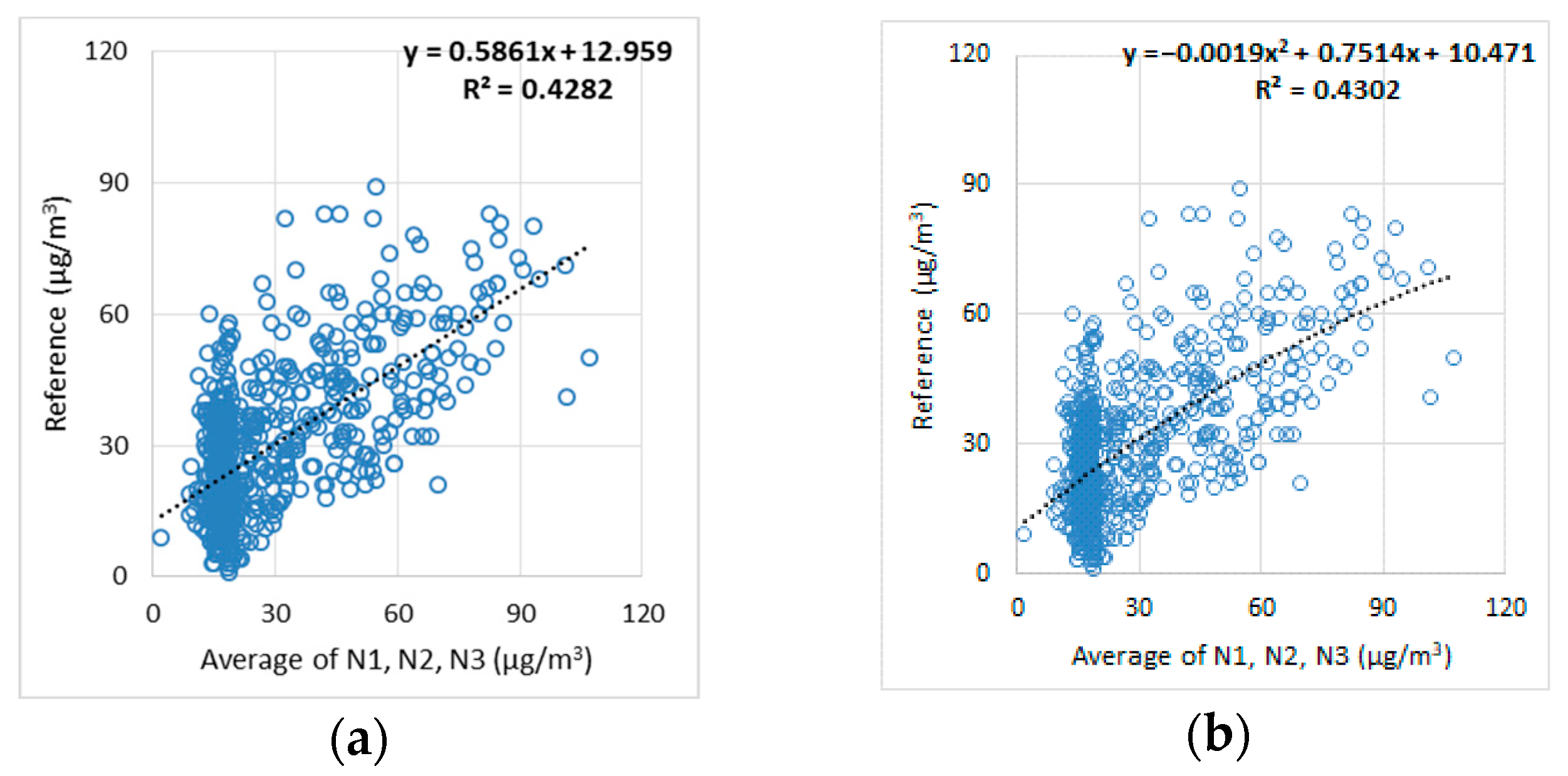
Figure 11 shows the average of the hourly nitrogen dioxide concentration measurements of the three low-cost sensors in relation to the reference measurements. Figure 12 shows both the simple linear regression scatter plot with the correlation degree and the nonlinear regression scatter plot with the polynomial equation of the correlation and the correlation degree, of the nitrogen dioxide concentration measurements.

Figure 11.
Time-series of the average of primary NO2 concentration measurements of the three nodes (N1, N2, N3) low-cost monitoring stations and reference instruments.

Figure 12.
Scatterplots of NO2 primary measurements. (a) Scatterplot of NO2 primary measurements of linear regression (LR) of average measurements (N1, N2, N3), (b) Scatterplot of NO2 primary measurements of nonlinear (NLR), (polynomial function 2nd degree) regression of average measurements (N1, N2, N3).
In order to evaluate the proposed methodology, the NLR was applied for each week of the selected period and the extracted coefficients were compared. This was conducted to ensure the time stability of the NLR methodology. Conclusively, to estimate the polynomial function the experiment was performed on a weekly basis. From the data of each week, both a polynomial function and the degree of correlation of the data emerged. The parameters of the rolling regression such as Alpha and Beta coefficients, Error, Correlation, and degree of correlation are shown, for the nitrogen dioxide concentrations, for the average value of the primary data of the three nitrogen dioxide sensors with the reference data in Table 3, and for the average value of the corrected data of the three nitrogen dioxide sensors with the reference data in Table 4.
Table 3.
Parameters of rolling regression between primary and reference measurements of NO2 for four weeks.
Table 4.
Parameters of rolling regression between corrected and reference measurements of NO2 for four weeks.
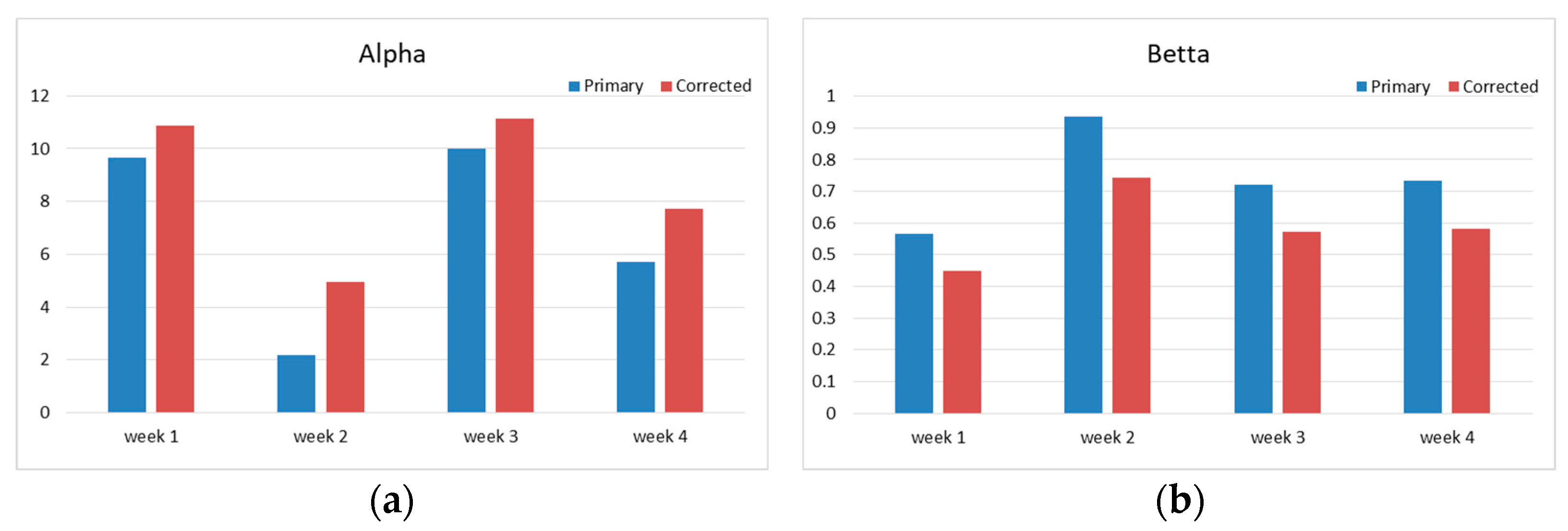
Figure 13 shows the coefficients (Alpha, Beta, Error, R2) both of the rolling regression of the average of the primary measurements of three nitrogen dioxide sensors and the reference, and the coefficients of the rolling regression of the average of the corrected by nonlinear regression measurements of three nitrogen dioxide sensors and the reference.

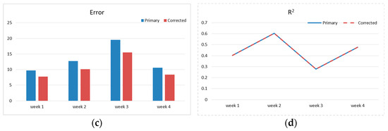
Figure 13.
Rolling regression coefficients of average of primary and average of corrected measurements (4 weeks) in respect to reference measurements of NO2, (a) Alpha coefficient of average of primary and average of corrected measurements in respect to reference measurements, (b) Beta coefficient of average of primary and average of corrected measurements in respect to reference measurements, (c) Error of average of primary and average of corrected measurements in respect to reference measurements, (d) Correlation degree (R2) coefficient of average of primary and average of corrected measurements in respect to reference measurements.
Τhe observations extracted from Figure 13 in relation to the corrected data, in terms of the coefficients of the rolling regression for a four-week period for nitrogen dioxide, show a slight increase in the Alpha coefficient, while the Beta coefficient shows a decrease, the Error shows aν average improvement of 20%, and the correlation coefficient (R2) remains stable.
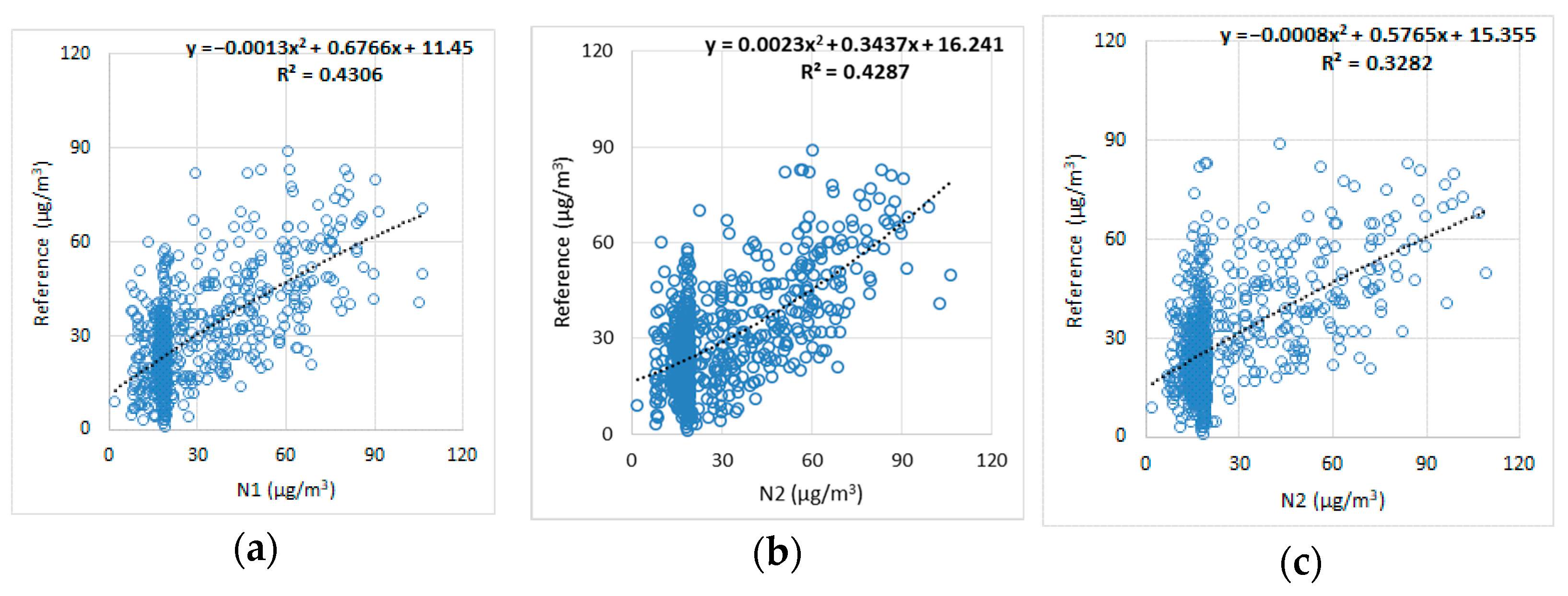
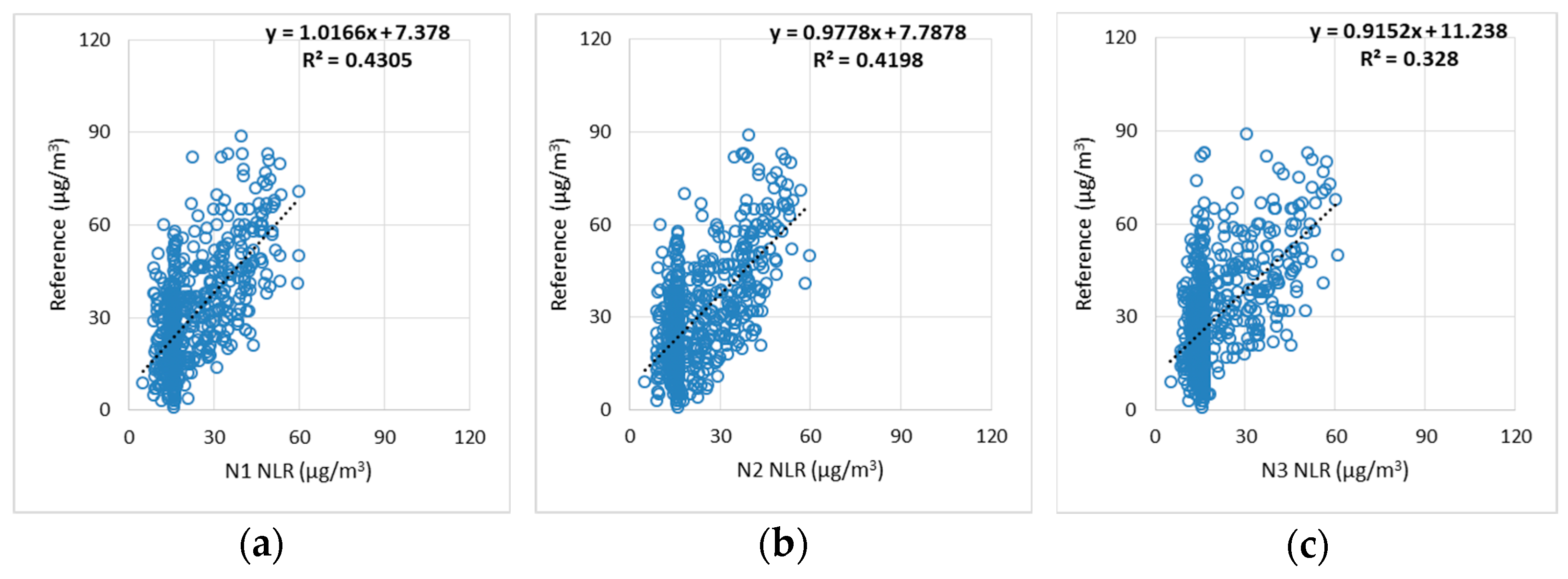
The extraction of the coefficients of the nonlinear correction function for nitrogen dioxide (NO2) was carried out as follows. From Figure 14 the square root of the average of the coefficients () of of N1, N2, N3 determines the value of the coefficient () of in the correction equation. The value of the coefficient () of of the correction equation can range from the maximum value that each coefficient () of shows in the scatter plots of the Figure 14 to their average value; the most appropriate value () of was chosen which gives the optimum effect on all three sensors. The coefficient () of the correction equation is obtained by taking the square root of the average of the coefficients () shown in the scatter plots of Figure 14.
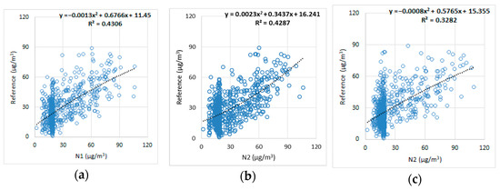
Figure 14.
Scatterplot of all NO2 primary measurements in respect to the reference measurements of nonlinear (NLR), (polynomial function 2nd degree) regression. (a) Scatterplot between primary of N1 and reference measurements of NO2 of nonlinear (NLR) regression, (b) Scatterplot between primary of N2 and reference measurements NO2 of nonlinear (NLR) regression, (c) Scatterplot between primary of N3 and reference measurements NO2 of nonlinear (NLR) regression.
The calculation of the polynomial function for the correction at the monthly level was done by co-estimating both the polynomial correlations from Figure 13 and Figure 14 and the correctness, evaluation, and reliability of the results with respect to the reference data. The polynomial function acting on the sensor data as a correction factor to the nitrogen dioxide gas pollutant concentration measurements of low-cost sensors is described in Equation (7)
where, , is the corrected concentration measurement of nitrogen dioxide and is the primary concentration measurement of nitrogen dioxide low-cost sensor.
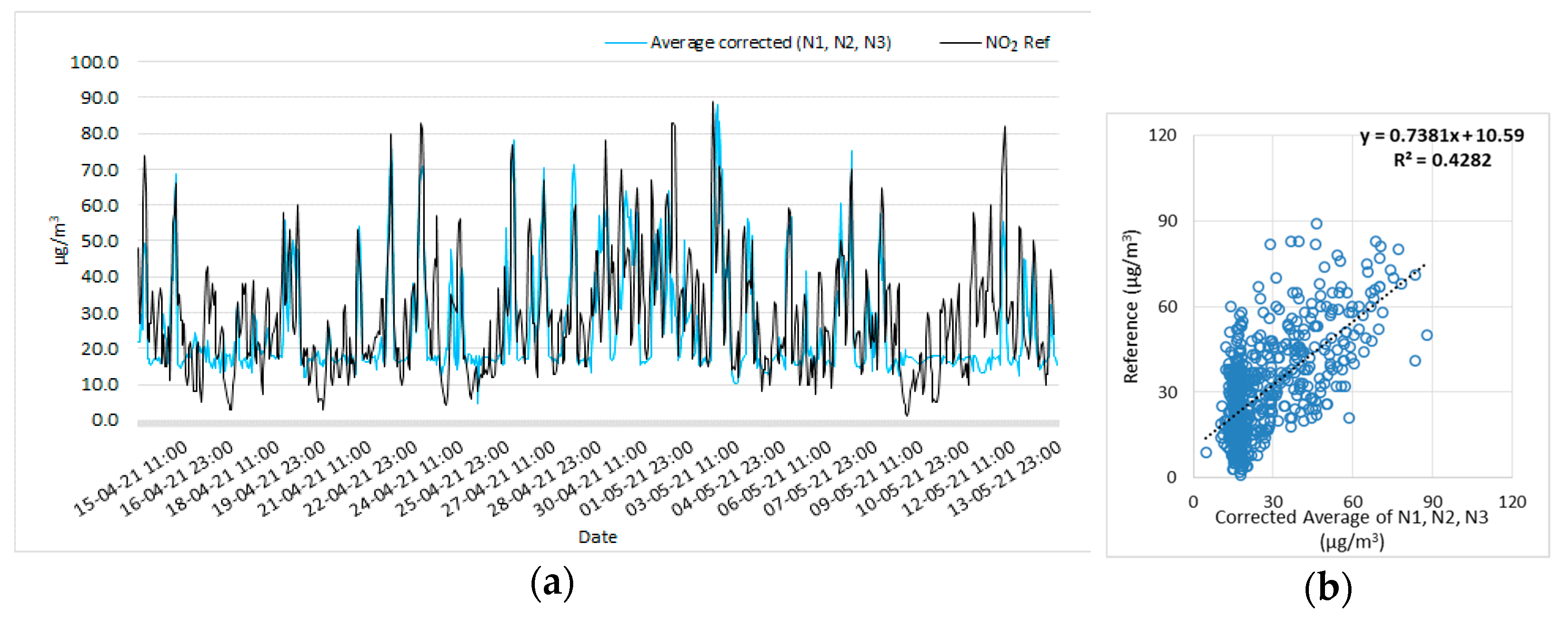
The polynomial function of Equation (7) was applied to the primary data of each low-cost nitrogen dioxide (NO2) sensor. Figure 15 shows the time series and scatter plot of the average of corrected measurements in respects to reference measurements. The scatter plots of corrected measurements in comparison with reference measurements for nitrogen dioxide concentrations are shown in Figure 16 for nodes N1, N2, N3, respectively.
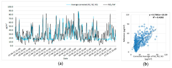
Figure 15.
Time-series and scatterplot of average of corrected NO2 measurements of N1, N2, N3, and reference measurements, (a) Time-series of average of corrected NO2 measurements of N1, N2, N3, and reference measurements, (b) Scatterplot of average of corrected NO2 measurements of N1, N2, N3 and reference measurements.
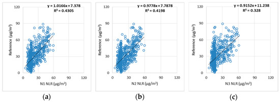
Figure 16.
Scatterplots of NO2 corrected measurements of N1, N2, N3 and reference measurements, (a) Scatterplot of NO2 corrected measurements of N1 and reference measurements, (b) Scatterplot of NO2 corrected measurements of N2 and reference measurements, (c) Scatterplot of NO2 corrected measurements of N3 and reference measurements.
3.3. Comparisson Results of RMSE, MAD, MAE Methods Evaluation
For evaluation of the results of the application of nonlinear regression to measurements of air pollutant concentration from low-cost sensors, the methods of Root Mean Square Error (RMSE), Mean Absolute Deviation (MAD), and Mean Absolute Error (MAE) were applied to both weekly and monthly measurement data. Data are reported for the primary and corrected (nonlinear regression) measurements for each low-cost sensor (ozone and nitrogen dioxide) relative to reference measurements.
Table 5 and Table 6 show the RMSE, MAD, and MAE results of both primary and corrected measurements for the three low-cost ozone (O3) sensors, in monthly and weekly measurements, respectively.
Table 5.
Monthly evaluation of O3 measurements via RMSE, MAD, MAE methods.
Table 6.
Weekly evaluation of O3 measurements via RMSE, MAD, MAE methods.
Table 7 and Table 8 show the RMSE, MAD, and MAE results of both primary and corrected measurements for the three low-cost nitrogen dioxide (NO2) sensors, in monthly and weekly measurements, respectively.
Table 7.
Monthly evaluation of NO2 measurements via RMSE, MAD, and MAE methods.
Table 8.
Weekly evaluation of NO2 measurements via RMSE, MAD, and MAE methods.
Observing Table 5 and Table 6 for ozone and Table 7 and Table 8 for nitrogen dioxide, on a weekly and monthly basis, as corrected data compared to the primary data, the following can be concluded. The degree of correlation decreases slightly, while an improvement is evident in both the MAD and MAE methods, as they show less divergence and error, which means that the corrected measurements are more realistic and reliable. Specifically, the improvements in the corrected measurements by nonlinear regression, according to the RMSE, MAD and MAE methods is shown for ozone, the monthly measurements (Table 5), the RMSE of 20% to 60%, the MAD of 10% to 24% and the MAE of 7% to 15%. The weekly measurements (Table 6), the RMSE of 17% to 86%, the MAD of 9% to 14% and the MAE of 3% to 9%. For nitrogen dioxide, the monthly measurements (Table 7) show RMSE of 3% to 28%, MAD of 9% to 60% and MAE of 4% to 25%. The weekly measurements (Table 8) show RMSE of 1% to 3%, MAD of 1% to 3% and MAE of 3% to 4%.
4. Discussion
The improvements in the methodology of nonlinear regression as correction factor show satisfactory results. In general, simple nonlinear regression models as correction factors in low-cost sensor measurements are not commonly found in the literature. Instead, many research papers have been published on correction models using random forest (RF), artificial neural networks (ANN), support vector machine (SVM), and support vector regression (SVR) techniques. These techniques have shown excellent results in improving measurements. As the platform presented here belongs to IoT devices, it is understood that such technologies are not typically supported by IoT devices. Given that the correction of the measurements has to be carried out at the monitoring station, which is based on an IoT device, with limited computing power, the application of correction by nonlinear regression is feasible, compared to other methods which require high processing power and cannot be underestimated by such devices.
The application of simple nonlinear regression (NLR) to measurement data from low-cost sensors, in particular electrochemical nitrogen dioxide and ozone sensors, shows that it can improve the measurements from these sensors to a certain extent.
The experiment was conducted using both weekly and monthly data. Concerning ozone, the weekly corrected data exhibited an improvement in the degree of correlation of up to 5% compared to the primary data, while the monthly corrected data showed an enhancement in the correlation coefficient of up to 4%. For nitrogen dioxide, the weekly corrected data demonstrated an increase in the correlation coefficient of up to 9% compared to the primary data, while the monthly corrected data indicated an improvement in the correlation coefficient of up to 2.5%.
The validation of the improvements are shows by the comparison results of the RMSE, MAD and MAE methods, According to Table 5 and Table 6 comparing the primary and corrected measurements in respect to reference measurements, for the monthly measurements of ozone, the RMSE shows an improvement of up to 60%, the MAD shows an improvement or up to 24% and the MAE shows an improvement of up to 15%. For the weekly measurements of ozone, the RMSE shows an improvement of up to 86%, the MAD shows an improvement of up to 14% and the MAE shows an improvement of up to 9%. According to the Table 7 and Table 8 comparing the primary and corrected measurements in respect to reference measurements, for the monthly measurements of nitrogen dioxide, the RMSE shows an improvement of up to 28%, MAD shows an improvement of up to 60% and MAE shows an improvement of up to 25%. For the weekly measurements for ozone, the RMSE shows an improvement of up to 3%, the MAD shows an improvement of up to 3% and the MAE shows an improvement pf up to 4%.
In addition, methodology scaling was followed to investigate the reliability of the corrected measurements through the nonlinear regression approach, which encompasses both time scaling and the seasonality scale.
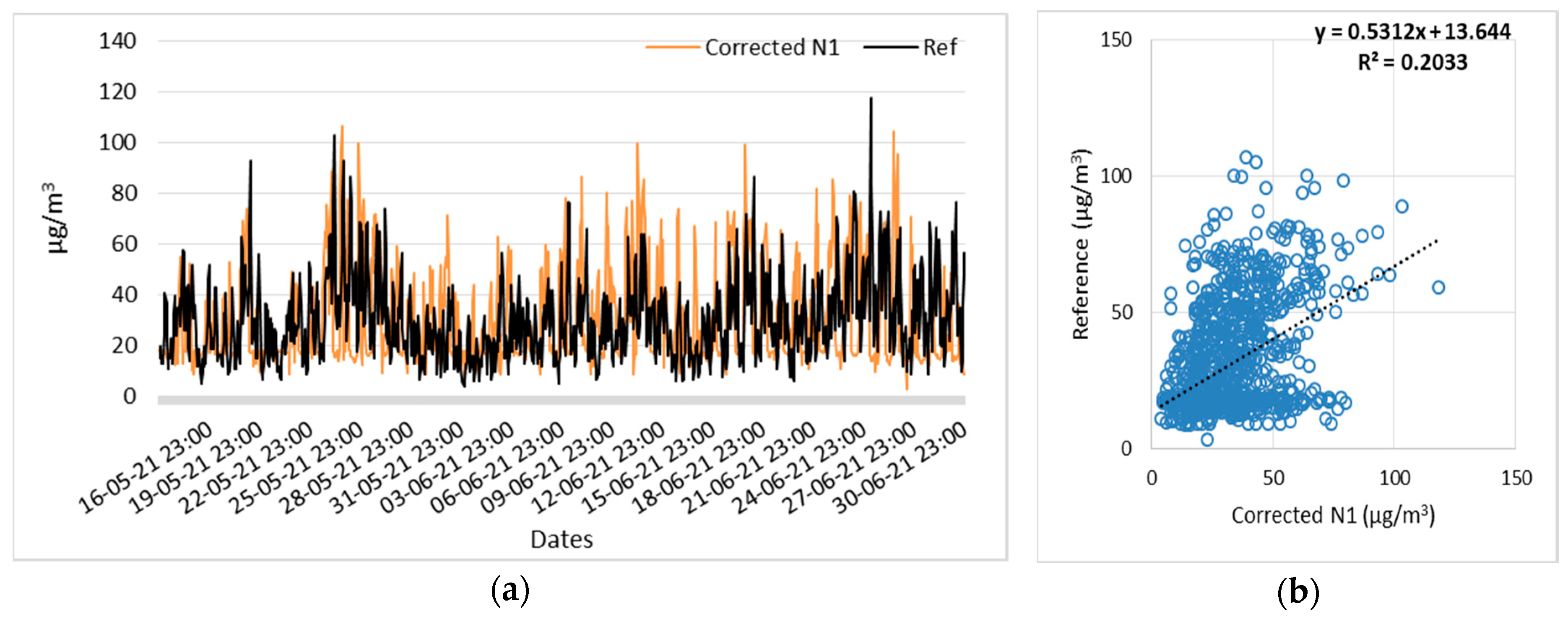
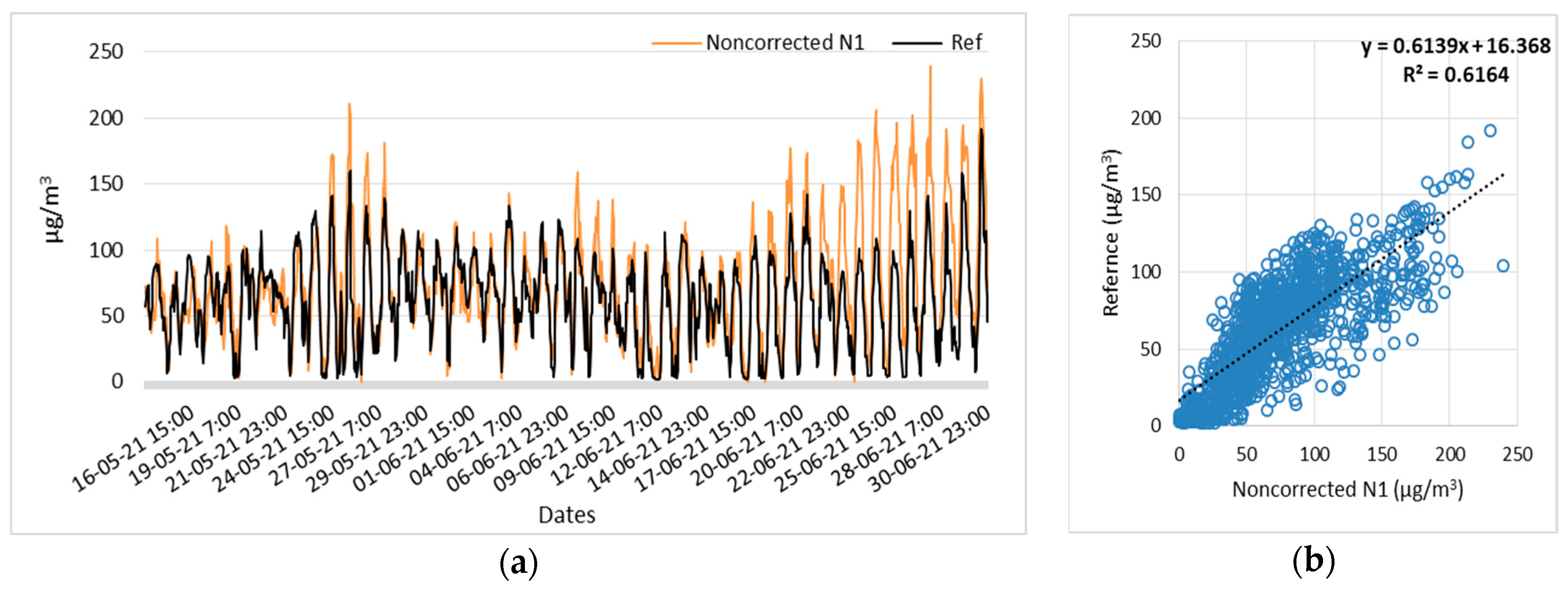
The evaluation of the time scaling of the experiment involved applying the nonlinear regression approach for a period of one and a half months following the main experiment (i.e., from 14 May 2021 to 31 June 2021) to all low-cost sensors. Indicative results are presented in the figures below. For simplicity and given that all nodes show high correlation with each other. Figure 17 shows the time-series and scatter plots of non-corrected NO2 measurements from node N1 and reference measurements, during the time period from 14 May 2021 to 31 June 2021. Correspondingly, Figure 18 shows the time-series and scatter plots of NO2 corrected measurements from N1 and reference measurements, for the time period of 14 May 2021 to 31 June 2021.
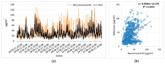
Figure 17.
Time-series and scatter plots of NO2 non-corrected measurements of node N1 and reference measurements, for the time period of 14 May 2021 to 31 June 2021. (a) Time series of N1 (NO2) non-corrected and reference measurements, (b) Scatterplot of N1 (NO2) non-corrected and reference measurements.

Figure 18.
Time-series and scatter plots of NO2 corrected measurements of node N1 and reference measurements, for the time period of 14 May 2021 to 31 June 2021. (a) Time series of N1 (NO2) corrected and reference measurements, (b) Scatterplot of N1 (NO2) corrected and reference measurements.
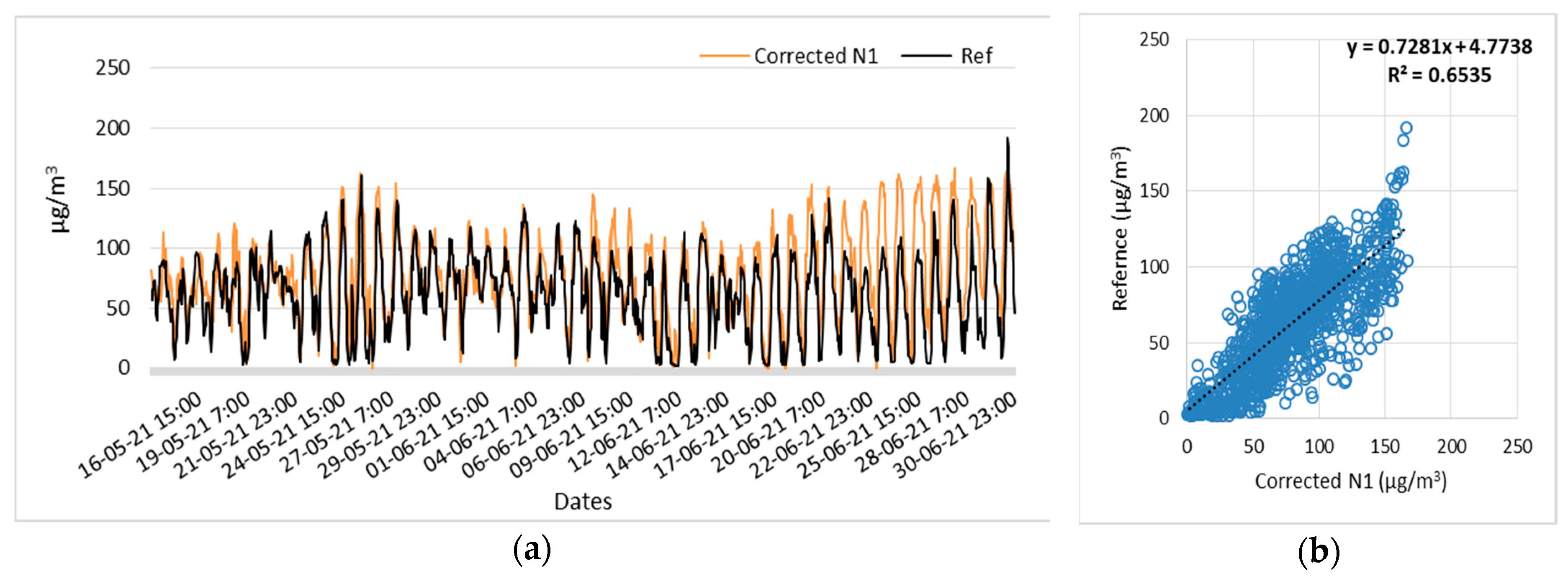
In fully compliance and correspondence, Figure 19 shows the time-series and scatter plots of O3 non-corrected measurements of node N1 and reference measurements, during the time period from 14 May 2021 to 31 June 2021. Respectively, Figure 20 shows the time-series and scatter plots of O3 corrected measurements of node N1 and reference measurements, during time period from 14 May 2021 to 31 June 2021.
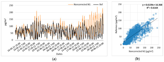
Figure 19.
Time-series and scatter plots of O3 non-corrected measurements of node N1 and reference measurements, for the time period of 14 May 2021 to 31 June 2021. (a) Time series of N1 (O3) non-corrected and reference measurements, (b) Scatterplot of N1 (O3) non-corrected and reference measurements.
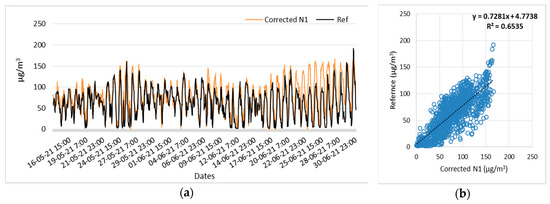
Figure 20.
Time-series and scatter plots of O3 corrected measurements of node N1 and reference measurements, for the time period from 14 May 2021 to 31 June 2021. (a) Time series of N1 (O3) corrected and reference measurements, (b) Scatterplot of N1 (O3) corrected and reference measurements.
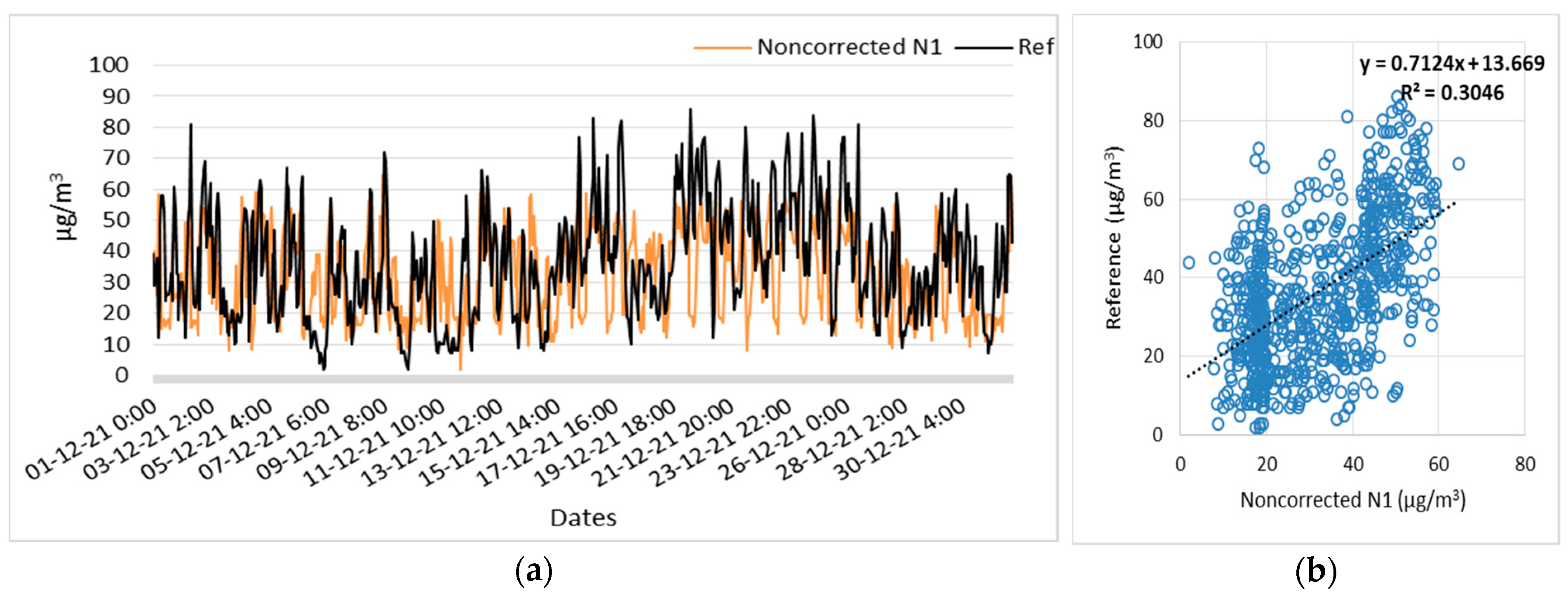
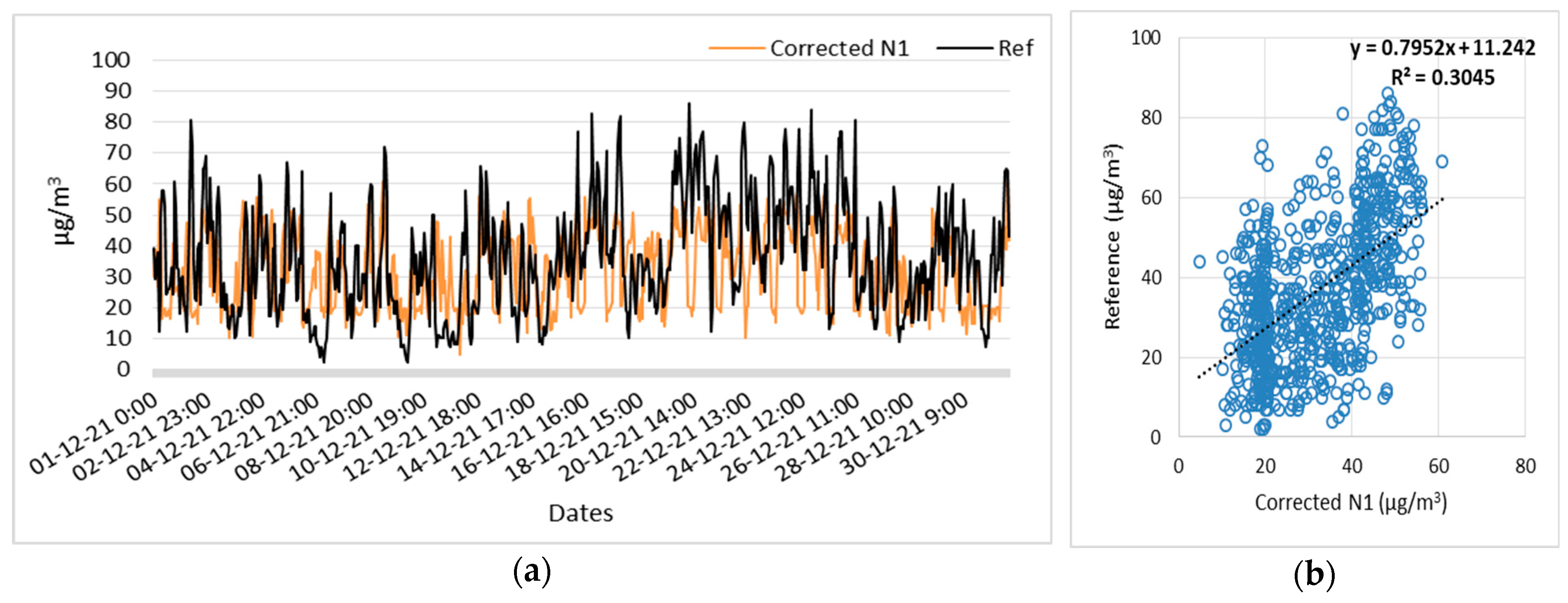
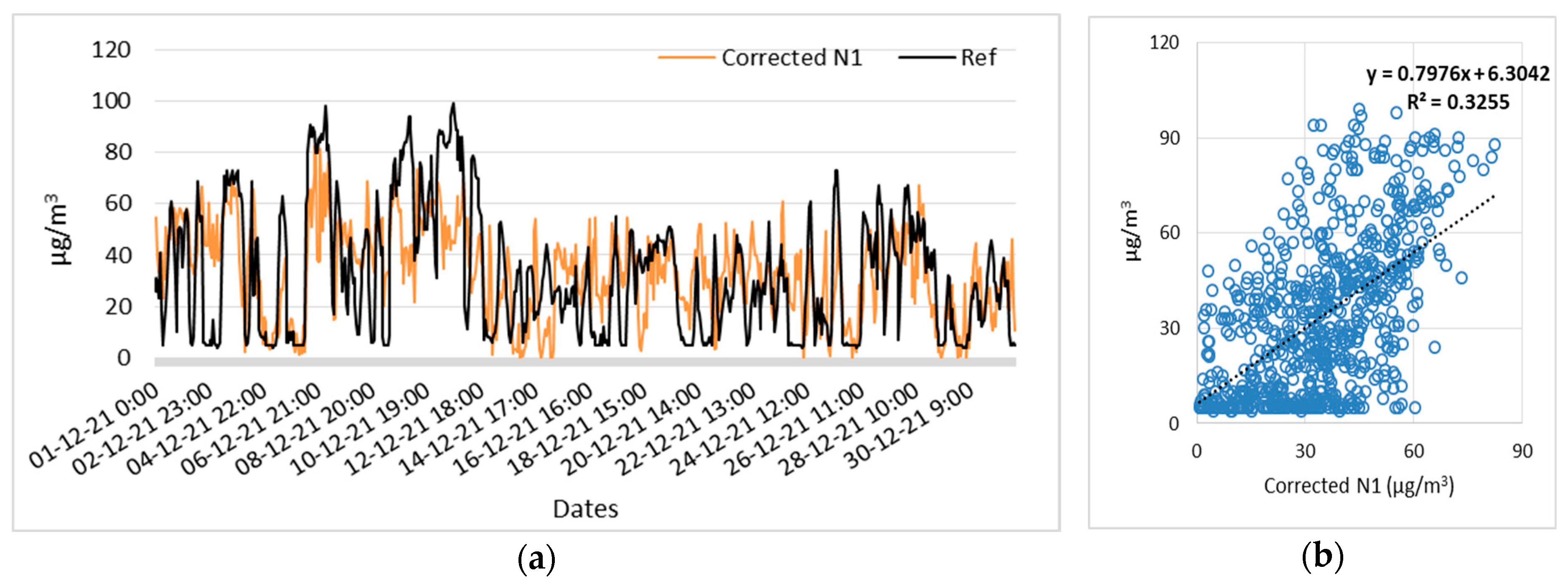
In order to determine whether seasonality affects the results, the nonlinear regression approach was applied during the winter month of December 2021 (i.e., from 1 December 2021 to 31 December 2021), to all low-cost sensors, where indicative results are shown in the figures below. Figure 21 shows the time-series and scatter plots of NO2 non-corrected measurements of node N1 and reference measurements, for the time period of 1 December 2021 to 31 December 2021. Figure 22 shows the corresponding time-series and scatter plots of NO2 corrected measurements for node N1 and reference measurements, for the time period from 1 December 2021 to 31 December 2021.

Figure 21.
Time-series and scatter plots of NO2 non-corrected measurements of node N1 and reference measurements, for the time period of 1 December 2021 to 31 December 2021. (a) Time series of N1 (NO2) non-corrected and reference measurements, (b) Scatterplot of N1 (NO2) non-corrected and reference measurements.
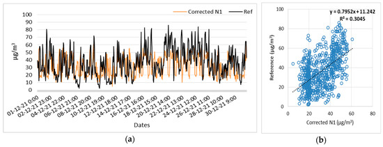
Figure 22.
Time-series and scatter plots of NO2 corrected measurements of node N1 and reference measurements, for the time period from 1 December 2021 to 31 December 2021. (a) Time series of N1 (NO2) corrected and reference measurements, (b) Scatterplot of N1 (NO2) corrected and reference measurements.
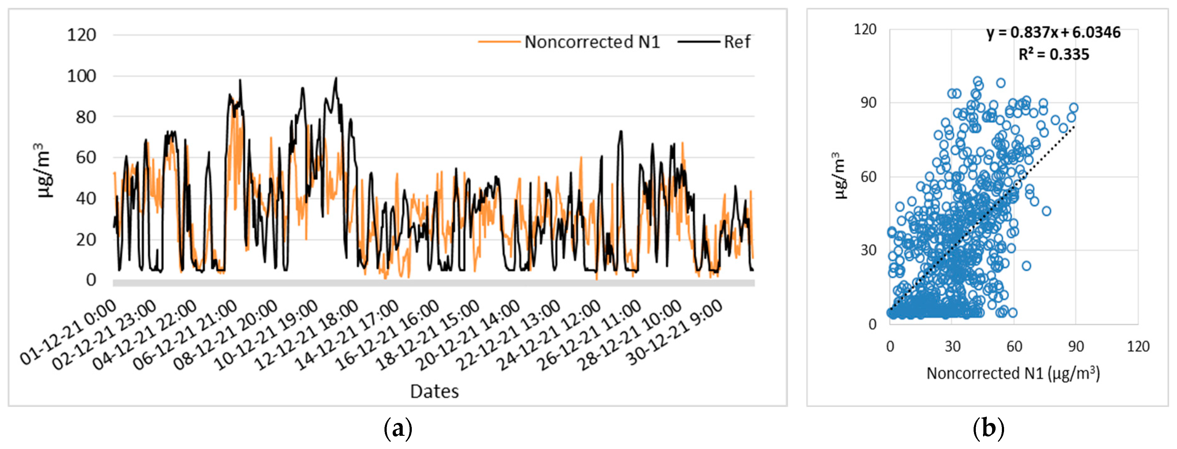
Figure 23 shows the time-series and scatter plots of O3 non-corrected measurements of node N1 and reference measurements for the time period of 1 December 2021 to 31 December 2021. Figure 24 shows the time-series and scatter plots of O3 corrected measurements of node N1 and reference measurements for the time period from 1 December 2021 to 31 December 2021.

Figure 23.
Time-series and scatter plots of O3 non-corrected measurements of node N1 and reference measurements for the time period from 1 December 2021 to 31 December 2021. (a) Time series of N1 (O3) non-corrected and reference measurements, (b) Scatterplot of N1 (O3) non-corrected and reference measurements.
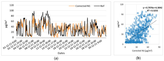
Figure 24.
Time-series and scatter plots of O3 corrected measurements of node N1 and reference measurements for the time period from 1 December 2021 to 31 December 2021. (a) Time series of N1 (O3) corrected and reference measurements, (b) Scatterplot of N1 (O3) corrected and reference measurements.
For reasons of completeness, Table 9 summarizes the above presented results and specifically the R2 and the , coefficients (of linear equation ) behavior before and after the application of the nonlinear regression model for all Nodes, N1, N2 and N3, in order to make clear the similar behavior of all sensing devices.
Table 9.
The behavior of R2 before and after the application of NLR during all periods of study, namely (14 April–13 May 2021, 14 May–30 July 2021, 1–31 December 2021).
Observing the results, the improvement does not appear directly from the degree of correlation between the corrected data and the reference data, but from the shift of the linear coefficients, after the application of nonlinear regression, which influence the effect of the correction. As a validation of the reliability of the correction, it is worth mentioning the results in the evaluation of the nonlinear regression method through the RMSE, MAD and MAE methods. The RMSE method showed small deviation between the primary and corrected values for both nitrogen dioxide and ozone sensors, as indicated by the tables for the monthly and weekly analysis of the results. In the MAD and MAE methods, the improvement is evident according to the results table. This correction achieved by the application of nonlinear regression has a direct effect on refining the measurements to be closer to the actual ones, which is achieved as demonstrated, for weekly measurements in particular, by Table 1 and Table 2, and Figure 5 for ozone, and Table 3 and Table 4, and Figure 13 for nitrogen dioxide, as well as by Figure 7 and Figure 8 for ozone and Figure 15 and Figure 16 for nitrogen dioxide, on a monthly basis. According to scaling methods, both time and seasonality (Table 9), the application of nonlinear regression, while not improving the correlation coefficient (R2), improves the linear coefficients. For both types of low-cost gas sensors (ozone and nitrogen dioxide), the analysis of the corrected measurements is carried out in accordance with, Table 2 and Figure 7 for ozone, and Table 4 and Figure 16 for nitrogen dioxide. This improvement affects the corrected measurements, making them closer to the reference measurements, indicating that the corrected measurements are more reliable.
5. Conclusions
In this work, the methodology of nonlinear regression as a correction factor in measurements from low-cost air pollutant sensors was presented. The advantage of this methodology is that it can be implemented in IoT devices, as it does not require high computational power. The proposed methodology proves excellent results, as the results indicate that a second-degree polynomial is adequate to show an improvement in the degree of correlation (R2) of up to 9% for ozone and up to 4% for nitrogen dioxide, while experiments with a higher degree polynomial were not adopted due to increased system complexity. The results of both scale methods demonstrate satisfactory performance, with corrected measurements closely aligning with reference measurements.
For the purpose of evaluating the results, the RMSE, MAD, and MAE methods were employed for both primary and corrected data. The RMSE method indicated a deviation between the primary and corrected results, suggesting the correction impact on the data. However, both the MAD and MAE methods showed an improvement in the corrected results, since for both types of air pollutant sensors both the mean absolute deviation and the mean absolute error show a smaller value in the corrected values compared to the reference values. In summary, Table 10 shows the improvements of average degree per method was used.
Table 10.
Average degree of improvements per method: RMSE, MAD, and MAE.
This means that the correction by the nonlinear regression method, although not directly improving the correlation degree, accelerates the results through the linear coefficients, with the final effect of reducing the occurrence of the reduction in both the MAD and MAE methods. In line with the previous values, the corrected values indicate closer alignment with the reference data and, therefore, increased reliability.
Nonlinear regression serves as an effective correction factor for data from low-cost sensors, feasible on both weekly and monthly bases. Notably, weekly correction demonstrates slightly superior performance in the corrected results, as evidenced by the RMSE, MAD, and MAE tables.
Given the global concern regarding air quality, expanding spatial coverage, especially in large urban areas, through air quality monitoring networks is crucial.
Author Contributions
Conceptualization, I.S. and I.C.; methodology, I.S., O.T., E.S., D.T. and I.C.; software, I.C.; validation, I.S., O.T., E.S., D.T. and I.C.; formal analysis, E.S., D.T. and I.C.; investigation, I.C.; resources, E.S., D.T. and I.C.; data curation, O.T. and I.C.; writing—original draft preparation, I.C., E.S. and D.T.; writing—review and editing, O.T., E.S., D.T. and I.S.; visualization, I.C.; supervision, D.T. and I.S.; project administration, I.S. All authors have read and agreed to the published version of the manuscript.
Funding
This research received no external funding.
Institutional Review Board Statement
Not applicable.
Informed Consent Statement
Not applicable.
Data Availability Statement
The original contributions presented in the study are included in the article, further inquiries can be directed to the corresponding author.
Conflicts of Interest
The authors declare no conflicts of interest.
References
- Kularatna, N.; Sudantha, B.H. An Environmental Air Pollution Monitoring System Based on the IEEE 1451 Standard for Low Cost Requirements. IEEE Sens. J. 2008, 8, 415–422. [Google Scholar] [CrossRef]
- Munir, S.; Mayfield, M.; Coca, D.; Jubb, S.A.; Osammor, O. Analysing the Performance of Low-Cost Air Quality Sensors, Their Drivers, Relative Benefits and Calibration in Cities—A Case Study in Sheffield. Environ. Monit. Assess. 2019, 191. [Google Scholar] [CrossRef]
- Clements, A.L.; Griswold, W.G.; Rs, A.; Johnston, J.E.; Herting, M.M.; Thorson, J.; Collier-Oxandale, A.; Hannigan, M. Low-Cost Air Quality Monitoring Tools: From Research to Practice (a Workshop Summary). Sensors 2017, 17, 2478. [Google Scholar] [CrossRef]
- Heimann, I.; Bright, V.B.; McLeod, M.W.; Mead, M.I.; Popoola, O.A.M.; Stewart, G.B.; Jones, R.L. Source Attribution of Air Pollution by Spatial Scale Separation Using High Spatial Density Networks of Low Cost Air Quality Sensors. Atmos. Environ. 2015, 113, 10–19. [Google Scholar] [CrossRef]
- Schneider, P.; Castell, N.; Vogt, M.; Dauge, F.R.; Lahoz, W.A.; Bartonova, A. Mapping Urban Air Quality in near Real-Time Using Observations from Low-Cost Sensors and Model Information. Environ. Int. 2017, 106, 234–247. [Google Scholar] [CrossRef]
- Austin, C.C.; Roberge, B.; Goyer, N. Cross-Sensitivities of Electrochemical Detectors Used to Monitor Worker Exposures to Airborne Contaminants: False Positive Responses in the Absence of Target Analytes. J. Environ. Monit. 2006, 8, 161–166. [Google Scholar] [CrossRef]
- Liu, D.; Zhang, Q.; Jiang, J.; Chen, D.-R. Performance Calibration of Low-Cost and Portable Particular Matter (PM) Sensors. J. Aerosol Sci. 2017, 112, 1–10. [Google Scholar] [CrossRef]
- Spinelle, L.; Gerboles, M.; Villani, M.G.; Aleixandre, M.; Bonavitacola, F. Field Calibration of a Cluster of Low-Cost Available Sensors for Air Quality Monitoring. Part A: Ozone and Nitrogen Dioxide. Sens. Actuators B Chem. 2015, 215, 249–257. [Google Scholar] [CrossRef]
- Popoola, O.A.M.; Stewart, G.B.; Mead, M.I.; Jones, R.L. Development of a Baseline-Temperature Correction Methodology for Electrochemical Sensors and Its Implications for Long-Term Stability. Atmos. Environ. 2016, 147, 330–343. [Google Scholar] [CrossRef]
- Castell, N.; Dauge, F.R.; Schneider, P.; Vogt, M.; Lerner, U.; Fishbain, B.; Broday, D.; Bartonova, A. Can Commercial Low-Cost Sensor Platforms Contribute to Air Quality Monitoring and Exposure Estimates? Environ. Int. 2017, 99, 293–302. [Google Scholar] [CrossRef]
- Maag, B.; Zhou, Z.; Thiele, L. A Survey on Sensor Calibration in Air Pollution Monitoring Deployments. IEEE Internet Things J. 2018, 5, 4857–4870. [Google Scholar] [CrossRef]
- Motlagh, N.H.; Lagerspetz, E.; Nurmi, P.; Li, X.; Varjonen, S.; Mineraud, J.; Siekkinen, M.; Rebeiro-Hargrave, A.; Hussein, T.; Petaja, T.; et al. Toward Massive Scale Air Quality Monitoring. IEEE Commun. Mag. 2020, 58, 54–59. [Google Scholar] [CrossRef]
- Borrego, C.; Costa, A.M.; Ginja, J.; Amorim, M.; Coutinho, M.; Karatzas, K.; Sioumis, T.; Katsifarakis, N.; Konstantinidis, K.; De Vito, S.; et al. Assessment of Air Quality Microsensors versus Reference Methods: The EuNetAir Joint Exercise. Atmos. Environ. 2016, 147, 246–263. [Google Scholar] [CrossRef]
- Han, P.; Mei, H.; Liu, D.; Zeng, N.; Tang, X.; Wang, Y.; Pan, Y. Calibrations of Low-Cost Air Pollution Monitoring Sensors for CO, NO2, O3, and SO2. Sensors 2021, 21, 256. [Google Scholar] [CrossRef]
- Christakis, I.; Hloupis, G.; Stavrakas, I.; Tsakiridis, O. Low Cost Sensor Implementation and Evaluation for Measuring NO2 and O3 Pollutants. In Proceedings of the 2020 9th International Conference on Modern Circuits and Systems Technologies (MOCAST), Bremen, Germany, 7–9 September 2020. [Google Scholar] [CrossRef]
- Lee, H.; Kang, J.; Kim, S.; Im, Y.; Yoo, S.; Lee, D. Long-Term Evaluation and Calibration of Low-Cost Particulate Matter (PM) Sensor. Sensors 2020, 20, 3617. [Google Scholar] [CrossRef]
- Kosmopoulos, G.; Salamalikis, V.; Pandis, S.N.; Yannopoulos, P.; Bloutsos, A.A.; Kazantzidis, A. Low-Cost Sensors for Measuring Airborne Particulate Matter: Field Evaluation and Calibration at a South-Eastern European Site. Sci. Total Environ. 2020, 748, 141396. [Google Scholar] [CrossRef]
- Migos, T.; Christakis, I.; Moutzouris, K.; Stavrakas, I. On the Evaluation of Low-Cost PM Sensors for Air Quality Estimation. In Proceedings of the 2019 8th International Conference on Modern Circuits and Systems Technologies, Thessaloniki, Greece, 13–15 May 2019. [Google Scholar] [CrossRef]
- Wei, P.; Ning, Z.; Ye, S.; Sun, L.; Yang, F.; Wong, K.; Westerdahl, D.; Louie, P. Impact Analysis of Temperature and Humidity Conditions on Electrochemical Sensor Response in Ambient Air Quality Monitoring. Sensors 2018, 18, 59. [Google Scholar] [CrossRef]
- Wang, Y.; Li, J.; Jing, H.; Zhang, Q.; Jiang, J.; Biswas, P. Laboratory Evaluation and Calibration of Three Low-Cost Particle Sensors for Particulate Matter Measurement. Aerosol Sci. Technol. 2015, 49, 1063–1077. [Google Scholar] [CrossRef]
- Masson, N.; Piedrahita, R.; Hannigan, M. Quantification Method for Electrolytic Sensors in Long-Term Monitoring of Ambient Air Quality. Sensors 2015, 15, 27283–27302. [Google Scholar] [CrossRef]
- Jiao, W.; Hagler, G.; Williams, R.; Sharpe, R.; Brown, R.; Garver, D.; Judge, R.; Caudill, M.; Rickard, J.; Davis, M.; et al. Community Air Sensor Network (CAIRSENSE) Project: Evaluation of Low-Cost Sensor Performance in a Suburban Environment in the Southeastern United States. Atmos. Meas. Tech. 2016, 9, 5281–5292. [Google Scholar] [CrossRef]
- Spinelle, L.; Gerboles, M.; Villani, M.G.; Aleixandre, M.; Bonavitacola, F. Field Calibration of a Cluster of Low-Cost Commercially Available Sensors for Air Quality Monitoring. Part B: NO, CO and CO2. Sens. Actuators B Chem. 2017, 238, 706–715. [Google Scholar] [CrossRef]
- Zheng, T.; Bergin, M.H.; Johnson, K.K.; Tripathi, S.N.; Shirodkar, S.; Landis, M.S.; Sutaria, R.; Carlson, D.E. Field Evaluation of Low-Cost Particulate Matter Sensors in High- and Low-Concentration Environments. Atmos. Meas. Tech. 2018, 11, 4823–4846. [Google Scholar] [CrossRef]
- Levy Zamora, M.; Buehler, C.; Lei, H.; Datta, A.; Xiong, F.; Gentner, D.R.; Koehler, K. Evaluating the Performance of Using Low-Cost Sensors to Calibrate for Cross-Sensitivities in a Multipollutant Network. ACS EST Eng. 2022, 2, 780–793. [Google Scholar] [CrossRef]
- Baron, R.; Saffell, J. Amperometric Gas Sensors as a Low Cost Emerging Technology Platform for Air Quality Monitoring Applications: A Review. ACS Sens. 2017, 2, 1553–1566. [Google Scholar] [CrossRef]
- Hofman, J.; Nikolaou, M.; Shantharam, S.P.; Stroobants, C.; Weijs, S.; La Manna, V.P. Distant Calibration of Low-Cost PM and NO2 Sensors; Evidence from Multiple Sensor Testbeds. Atmos. Pollut. Res. 2022, 13, 101246. [Google Scholar] [CrossRef]
- Karagulian, F.; Barbiere, M.; Kotsev, A.; Spinelle, L.; Gerboles, M.; Lagler, F.; Redon, N.; Crunaire, S.; Borowiak, A. Review of the Performance of Low-Cost Sensors for Air Quality Monitoring. Atmosphere 2019, 10, 506. [Google Scholar] [CrossRef]
- Ratingen, S.V.; Vonk, J.; Blokhuis, C.; Wesseling, J.; Tielemans, E.; Weijers, E. Seasonal Influence on the Performance of Low-Cost NO2 Sensor Calibrations. Sensors 2021, 21, 7919. [Google Scholar] [CrossRef]
- Aula, K.; Lagerspetz, E.; Nurmi, P.; Tarkoma, S. Evaluation of Low-Cost Air Quality Sensor Calibration Models. ACM Trans. Sens. Netw. 2022, 18, 1–32. [Google Scholar] [CrossRef]
- Suriano, D.; Penza, M. Assessment of the Performance of a Low-Cost Air Quality Monitor in an Indoor Environment through Different Calibration Models. Atmosphere 2022, 13, 567. [Google Scholar] [CrossRef]
- Kureshi, R.R.; Mishra, B.K.; Thakker, D.; John, R.; Walker, A.; Simpson, S.; Thakkar, N.; Wante, A.K. Data-Driven Techniques for Low-Cost Sensor Selection and Calibration for the Use Case of Air Quality Monitoring. Sensors 2022, 22, 1093. [Google Scholar] [CrossRef]
- Christakis, I.; Tsakiridis, O.; Kandris, D.; Stavrakas, I. A Kalman Filter Scheme for the Optimization of Low-Cost Gas Sensor Measurements. Electronics 2024, 13, 25. [Google Scholar] [CrossRef]
- Christakis, I.; Sarri, E.; Tsakiridis, O.; Stavrakas, I. Investigation of LASSO Regression Method as a Correction Measurements’ Factor for Low-Cost Air Quality Sensors. Signals 2024, 5, 60–86. [Google Scholar] [CrossRef]
- Christakis, I.; Sarri, E.; Tsakiridis, O.; Stavrakas, I. Identification of the Safe Variation Limits for the Optimization of the Measurements in Low-Cost Electrochemical Air Quality Sensors. Electrochem 2024, 5, 1–28. [Google Scholar] [CrossRef]
- Li, J.; Hauryliuk, A.; Malings, C.; Eilenberg, S.R.; Subramanian, R.; Presto, A.A. Characterizing the Aging of Alphasense NO2 Sensors in Long-Term Field Deployments. ACS Sens. 2021, 6, 2952–2959. [Google Scholar] [CrossRef]
- Christakis, I.; Tsakiridis, O.; Kandris, D.; Stavrakas, I. Air Pollution Monitoring via Wireless Sensor Networks: The Investigation and Correction of the Aging Behavior of Electrochemical Gaseous Pollutant Sensors. Electronics 2023, 12, 1842. [Google Scholar] [CrossRef]
- Brienza, S.; Galli, A.; Anastasi, G.; Bruschi, P. A Low-Cost Sensing System for Cooperative Air Quality Monitoring in Urban Areas. Sensors 2015, 15, 12242–12259. [Google Scholar] [CrossRef]
- Kortoçi, P.; Motlagh, N.H.; Zaidan, M.A.; Fung, P.L.; Varjonen, S.; Rebeiro-Hargrave, A.; Niemi, J.V.; Nurmi, P.; Hussein, T.; Petäjä, T.; et al. Air Pollution Exposure Monitoring Using Portable Low-Cost Air Quality Sensors. Smart Health 2021, 23, 100241. [Google Scholar] [CrossRef]
- Christakis, I.; Hloupis, G.; Tsakiridis, O.; Stavrakas, I. Integrated Open Source Air Quality Monitoring Platform. In Proceedings of the 2022 11th International Conference on Modern Circuits and Systems Technologies, Bremen, Germany, 8–10 June 2022. [Google Scholar] [CrossRef]
- Koziel, S.; Pietrenko-Dabrowska, A.; Wojcikowski, M.; Pankiewicz, B. On Memory-Based Precise Calibration of Cost-Efficient NO2 Sensor Using Artificial Intelligence and Global Response Correction. Knowl. Based Syst. 2024, 290, 111564. [Google Scholar] [CrossRef]
- Poupry, S.; Medjaher, K.; Béler, C. Data Reliability and Fault Diagnostic for Air Quality Monitoring Station Based on Low Cost Sensors and Active Redundancy. Measurement 2023, 223, 113800. [Google Scholar] [CrossRef]
- Patton, A.; Datta, A.; Zamora, M.L.; Buehler, C.; Xiong, F.; Gentner, D.R.; Koehler, K. Non-Linear Probabilistic Calibration of Low-Cost Environmental Air Pollution Sensor Networks for Neighborhood Level Spatiotemporal Exposure Assessment. J. Expo. Sci. Environ. Epidemiol. 2022, 32, 908–916. [Google Scholar] [CrossRef]
- Sá, J.P.; Chojer, H.; Branco, P.T.B.S.; Alvim-Ferraz, M.C.M.; Martins, F.G.; Sousa, S.I.V. Two Step Calibration Method for Ozone Low-Cost Sensor: Field Experiences with the UrbanSense DCUs. J. Environ. Manag. 2023, 328, 116910. [Google Scholar] [CrossRef] [PubMed]
- Air Pollution Measurement Data. Ministry of Environment & Energy, Greece. Available online: https://ypen.gov.gr/perivallon/poiotita-tis-atmosfairas/dedomena-metriseon-atmosfairikis-rypansis/ (accessed on 14 December 2023).
- AlphaSense NO2-B43F. Available online: https://ametekcdn.azureedge.net/mediafiles/project/oneweb/oneweb/alphasense/products/datasheets/alphasense_no2-b43f_datasheet_en_1.pdf?revision:95cdfc22-824f-482a-b26d-d7f2f4688ea8 (accessed on 28 February 2024).
- AlphaSense OX-B431. Available online: https://ametekcdn.azureedge.net/mediafiles/project/oneweb/oneweb/alphasense/products/datasheets/alphasense_ox-b431_datasheet_en_1.pdf?revision:afe72812-8a0a-4a30-8e56-1b7047c532ab (accessed on 28 February 2024).
- Alphasense Application Note AAN 803-01 Correcting for Background Currents in Four Electrode Toxic Gas Sensors. 2014. Available online: https://zueriluft.ch/makezurich/AAN803.pdf (accessed on 30 March 2024).


Disclaimer/Publisher’s Note: The statements, opinions and data contained in all publications are solely those of the individual author(s) and contributor(s) and not of MDPI and/or the editor(s). MDPI and/or the editor(s) disclaim responsibility for any injury to people or property resulting from any ideas, methods, instructions or products referred to in the content. |
© 2024 by the authors. Licensee MDPI, Basel, Switzerland. This article is an open access article distributed under the terms and conditions of the Creative Commons Attribution (CC BY) license (https://creativecommons.org/licenses/by/4.0/).