Abstract
The lung is one of the most vital organs in the human body, and its condition is closely correlated with overall health. Electrical impedance tomography (EIT), as a biomedical imaging technique, often produces low-quality reconstructed images due to its inherent ill-posedness in solving the inverse problem. To address this issue, this paper proposes a soft-threshold region segmentation algorithm with a relaxation factor. This algorithm segments the reconstructed lung images into internal regions, edge regions, and background regions, resulting in clearer boundaries in the reconstructed images. This facilitates the intuitive identification of regions of interest by healthcare professionals. Additionally, this segmentation algorithm is suitably combined with a dimension-reduced Tikhonov regularization algorithm. By utilizing the joint capabilities of these algorithms, the partition points belonging to the background region can be excluded from the sought grayscale vector, thereby improving the ill-posedness of the image reconstruction process and enhancing the quality of image reconstruction. Finally, a 16-electrode human lung EIT simulation model is established for the thoracic region and verified through simulation. Experimental validation is conducted using a human lung tank simulation platform to further demonstrate the effectiveness of the proposed method.
1. Introduction
The lung is one of the most important organs in the thoracic cavity of the human body. Lung diseases are common and significant health concerns, particularly due to factors such as air pollution, an aging population, and the impact of conditions like COVID-19 [1,2,3]. Therefore, accurate, safe, and convenient monitoring of lung conditions is of great significance for the diagnosis and control of pulmonary diseases [4]. As a visualization technique, electrical impedance tomography (EIT) has gradually been commercialized and introduced into medical applications. EIT measures electrical signals at the boundary of the measured field using an array of electrodes and then performs an inversion reconstruction to obtain the distribution of electrical properties such as conductivity and relative permittivity within the field. The reconstructed information is presented in the form of visual images. EIT offers advantages such as non-invasiveness, portability, low cost, and continuous monitoring [5]. It has become an increasingly important imaging modality, providing significant advantages over traditional imaging techniques such as computed tomography (CT) and magnetic resonance imaging (MRI) in early screening, diagnosis, and bedside monitoring of lung diseases [4,5,6].
As a crucial component in the EIT system, the solution of the inverse problem (i.e., the image reconstruction process) largely determines the imaging performance of the EIT system [7]. However, the EIT image reconstruction process often suffers from ill-posedness [8]. Specifically, the number of measurement data obtained from the boundary electrodes is much smaller than the number of unknown reconstruction pixels. In other words, the number of equations in the system of equations established during the inverse problem solution is far less than the number of unknowns, resulting in severe ill-posedness in the image reconstruction process [8,9]. Due to the ill-posed nature of EIT, the original reconstructed EIT images obtained using image reconstruction algorithms often lack clear boundaries. Consequently, it becomes challenging to accurately identify the regions of interest (ROIs) in the lungs and determine the contours of conductivity variations during the respiratory process. Accurate identification of the lung region in the reconstructed image plays a crucial role in the analysis and diagnosis of pulmonary diseases. For example, in the context of acute respiratory distress syndrome titration, it is necessary to obtain regional-volume-dependent parameters and quantify the global inhomogeneity index through image analysis [10].
Extensive research has been conducted by various research teams over the past two decades to address the issues encountered in the EIT image reconstruction process. On one hand, some research teams have focused on optimizing imaging algorithms. They have improved and developed multiple optimized imaging algorithms based on classical algorithms, such as the linear back projection (LBP) algorithm [11], Landweber iteration algorithm [12], and Tikhonov regularization algorithm [13,14], to mitigate the ill-posedness problem in the image reconstruction process. For example, Yan et al. [9] proposed an iterative reconstruction algorithm with adaptive regularization parameters for the target and background. Iteration termination was determined based on the reversal of the trend in residual norms. Ding et al. [8] introduced fuzzy linear programming into EIT imaging and established a novel fuzzy optimization model, obtaining the optimal solution using fuzzy linear programming with constrained coefficients. Shi et al. [15] proposed a new method that combines the Gikhmanov regularization method with the wavelet framework, which exhibits significant advantages in enhancing the sparsity of the solution. Liu et al. [16] presented a spatio-temporal structure-aware sparse Bayesian learning (SA-SBL) framework that explores and exploits intra-frame spatial clustering and inter-frame temporal continuity in an unsupervised manner, using a hierarchical Bayesian model and structure-aware priors. Chen et al. [17] introduced a novel spatio-temporal total variation regularization method to utilize the sparsity in 4D space and time and adopted voxel-to-voxel cross-correlation to measure the flow profile. Song et al. [18] proposed a nonlinear weighted anisotropic total variation (NWATV) regularization technique that incorporates internal inhomogeneity information into the EIT reconstruction process, successfully preserving and improving the characteristics of internal inhomogeneity. Gong et al. [19] considered modifying the TV regularization term with higher-order differential operators during the image reconstruction process and applied the total generalized variation (TGV) regularization to the finite element model (FEM) framework for EIT reconstruction, thereby improving the ill-posedness of the inverse problem. Shi et al. [20] proposed an improved non-convex-L1-norm-penalized total generalized variation (NCP-TGV) model to solve the inverse problem. They developed an iteratively reweighted L1 algorithm that transforms the non-convex model into a convex function, offering advantages in reducing staircase effects and preserving edges simultaneously.
On the other hand, some research teams have integrated computer vision and image processing techniques with EIT technology to process the raw reconstructed EIT images using methods like image segmentation, thereby obtaining more accurate regions of interest (ROIs). For example, Guo et al. [21] developed a novel strategy for ECT image reconstruction that combines images reconstructed using two different algorithms through image segmentation methods. This approach retains the advantages of each algorithm for specific imaging regions and improves the overall image reconstruction quality. Borgmann et al. [22] proposed a method to estimate lung area using functional tidal images or active contour methods, achieving accurate estimation of lung area through image processing. Khambampati et al. [23] introduced the Otsu thresholding method for the automatic detection of ROIs and used a nonlinear diffusion imaging method to simultaneously estimate the initial values and differences in conductivity. Different regularization schemes were applied to the background and ROIs to improve image reconstruction performance. Arshad et al. [24] proposed a standardized method for evaluating and comparing cardiac EIT images based on automated segmentation. They designed an automated solution to segment and extract features from the images, accurately capturing various cardiac ROIs and extracting features. Ko et al. [10] developed an automatic lung segmentation model using deep learning with the U-Net architecture. This model enables automatic, robust, and fast lung segmentation in EIT images without the need for prior information, thus defining appropriate ROIs.
However, due to the “soft field” effect and the ill-posedness of the inverse problem in EIT, the performance of image reconstruction algorithms is still far from perfect. Therefore, more efforts are needed to develop better reconstruction algorithms. In this paper, we propose a region segmentation algorithm with a relaxation factor based on the traditional maximum entropy thresholding method. By adjusting the relaxation factor parameter, we can control the degree of preserving edge artifacts in the reconstructed image. This algorithm not only serves as an effective post-processing method for identifying regions of interest in EIT images but also complements the reduced-order Tikhonov regularization algorithm. Based on the segmentation results obtained from the soft-threshold region segmentation algorithm, the background region unrelated to the regions of interest is excluded from the solution process in the reduced-order operation. The pixel values belonging to the background region are removed from the solution process. By reducing the number of unknowns while keeping the number of equations in the inverse problem unchanged, the ill-posedness of the image reconstruction problem is improved, ultimately leading to higher-quality reconstructed images.
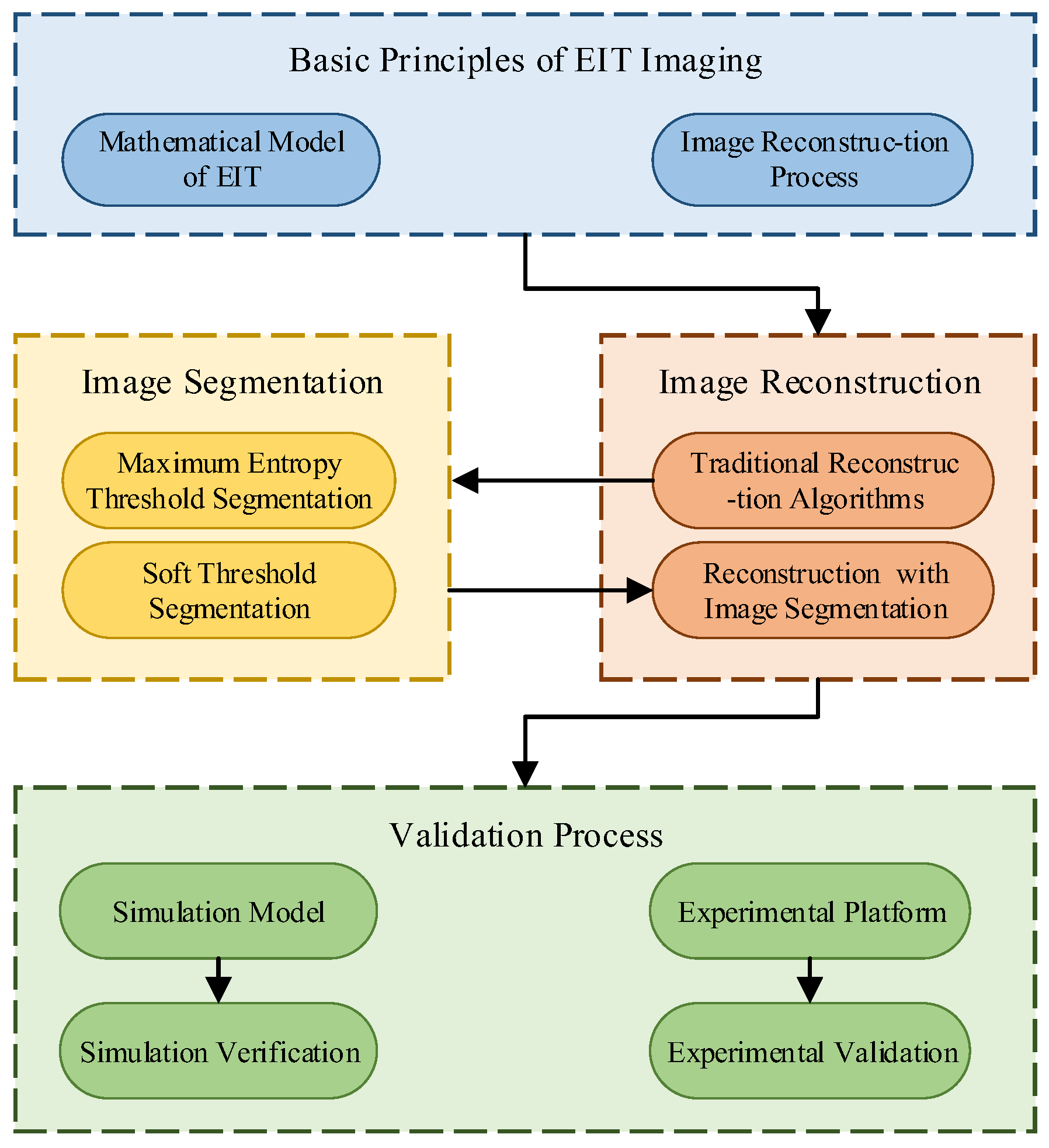
The structure of this paper is organized as follows: Firstly, Section 2 analyzes the basic principles of EIT imaging, establishes the mathematical model of EIT imaging, and analyzes the process of EIT image reconstruction. Then, in Section 3, image segmentation is applied to extract the region of interest for EIT, utilizing the maximum entropy threshold image segmentation algorithm and the soft-threshold segmentation algorithm. Subsequently, Section 4 proposes an image reconstruction algorithm based on image segmentation. In Section 5, a human chest 16-electrode EIT simulation model is established for simulation verification. Finally, in Section 6, an experimental platform for human lung electrical impedance tomography is constructed for experimental validation. The quantitatively calculated evaluation metrics show that the methods proposed in this paper can achieve better-reconstructed images. The schematic diagram of the paper’s structure is shown in Figure 1.
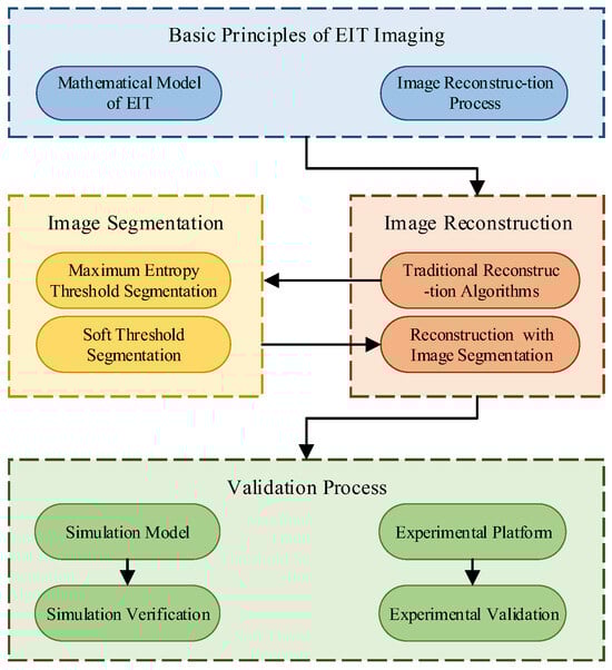
Figure 1.
Article structure schematic.
2. EIT Imaging Basic Principles
2.1. Mathematical Model of EIT Imaging
EIT technology is based on electromagnetic field theory, and the mathematical model of the electrical impedance tomography sensor, based on the differential form of Maxwell’s equations, can be described as follows:
In the above equation, E represents the electric field intensity, H represents the magnetic field intensity, J represents the current density, D represents the charge density, ϕ represents the electric potential distribution function, σ represents the conductivity, and ε represents the absolute permittivity.
When an excitation signal with a frequency of ω is applied to the measured field domain Ω, the electric field intensity can be expressed as E = Ê ejωt. Substituting this into Equation (1) yields:
Taking the divergence of both sides of Equation (2), we can obtain the following:
For the mathematical model of the sensitivity field in electrical impedance tomography (EIT), a unique solution exists when boundary conditions are applied to the field domain. The boundary condition utilized in this article is as follows:
In the above equation, n represents the outward normal unit vector of the boundary ∂Ω, and J denotes the injected current density on the boundary ∂Ω of the measured field Ω. For a given conductivity distribution σ, the specification of the boundary current density determines the measured voltage. The relationship between the conductivity distribution, current density, and boundary voltage measurements can be described as a nonlinear equation as follows:
where U is the boundary voltage measurement at the electrodes. The expression for the change in boundary voltage measurements under the perturbation of conductivity distribution Δσ can be given by the following equation:
By ignoring higher-order terms O((Δσ)2), the equation can be simplified to a linear form as follows:
Discretization of the above equation can further yield the following:
In the above equation, F is the n × 1 normalized boundary measurement difference, g is the m × 1 reconstructed image grayscale vector, and S is the n × m sensitivity matrix calculated based on Geselowitz’s sensitivity theorem [25]. m is the number of discretized elements, and n is the number of independent boundary measurements. Snm is the element at position (n,m) in S, with its calculation formula given as follows:
where ∇ϕm(Ii) is the potential at the mth pixel when the ith pair of electrodes injects current Ii, and ∇ϕm(Ij) is the potential at the mth pixel when the jth pair of electrodes injects current Ij.
This paper uses the finite element method to solve the forward problem of simulated boundary voltages and calculates the sensitivity matrix using COMSOL Multiphysics 5.6 software and MATLAB 2019 software. COMSOL Multiphysics, developed by Sweden’s COMSOL Group (Stockholm, Sweden), is an advanced numerical simulation software based on the finite element method. It simulates real physical phenomena by solving partial differential equations or systems of partial differential equations and has widespread applications in the field of electromagnetic field simulation.
2.2. EIT Image Reconstruction
EIT image reconstruction research is focused on the inverse problem. Based on the established simplified EIT model, the mathematical expression for the EIT inverse problem can be derived as follows:
In the above equation, S−1 represents the generalized inverse matrix of the m × n normalized sensitivity matrix. In most EIT systems, since m >> n, it is not possible to directly compute S−1. This fact highlights the ill-posed nature of the EIT image reconstruction process from another perspective.
The Tikhonov regularization algorithm, which is discussed in this paper, aims to mitigate the discontinuity in solving inverse problems through the L2 norm regularization and introduce prior information of the image for improving the stability of the solution. This optimization process helps to enhance the solution of ill-posed inverse problems. The mathematical expression of the Tikhonov regularization algorithm is given as follows:
In the above equation, α represents the regularization parameter, which plays a role in adjusting the weight of regularization. If α is too small, the regularization constraint cannot effectively control the solution. However, if α is too large, it may cause significant deviation between the reconstructed image and the true image. In this paper, the L-curve method [26] is employed to determine the optimal value of α. Therefore, for the original Tikhonov algorithm mentioned below, the regularization parameter is 0.00004. Meanwhile, the literature [9] suggests that a smaller regularization parameter should be used for the target area of imaging to enhance the detail reconstruction capability of the target area. Consequently, for the reduced-order Tikhonov algorithm, the regularization parameter used for the target area is 0.000025. In the equation, L represents the regularization operator, typically taken as the identity matrix E. Consequently, the regularized solution g can be obtained as follows:
3. EIT Region of Interest Image Segmentation Methods
3.1. Maximum Entropy Threshold Image Segmentation Method
In EIT image reconstruction, there is often no clear boundary between the region of interest and the background. In order to accurately identify the lung region in the reconstructed EIT image, image segmentation techniques have been introduced in this study. The purpose is to determine the position of the lung in the reconstructed image and obtain an easily identifiable lung area image. Taking the maximum entropy thresholding image segmentation as an example, it is a type of threshold-based segmentation method that can partition an image into multiple subregions with similar properties. It has been widely applied in image analysis and object recognition [27].
The maximum entropy thresholding method divides the image into regions of interest and background, where the threshold that maximizes the sum of the target entropy and background entropy is considered the optimal segmentation threshold. The conventional method of thresholding using one-dimensional grayscale histograms does not consider spatial information of the image and is susceptible to noise interference [28]. In this paper, the two-dimensional maximum entropy thresholding method considering both the pixel grayscale value and its neighborhood average grayscale value is used as an example. For an image of size N × M and grayscale levels L, the probability expression for the image’s binary tuple (i, j) is as follows:
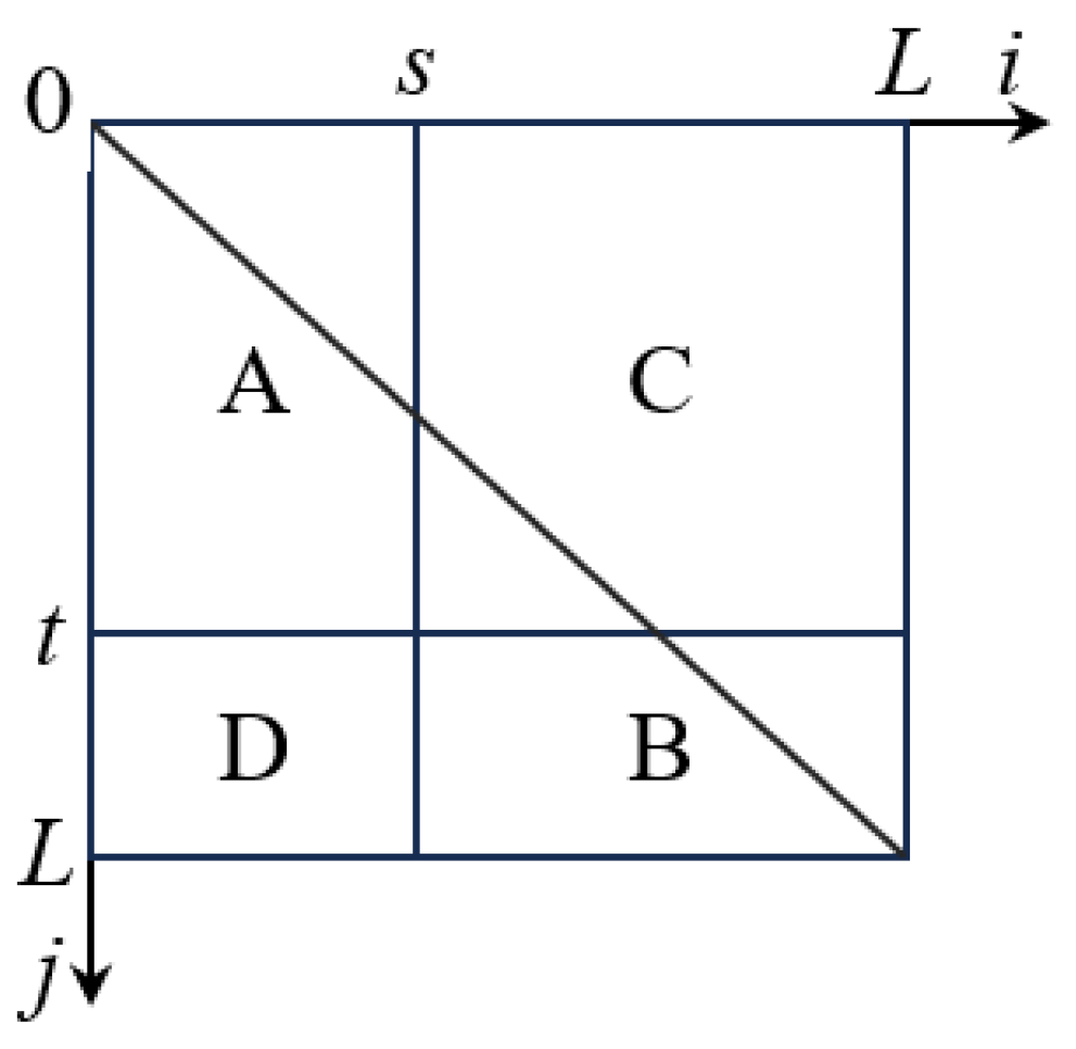
In the above equation, 0 ≤ i, j ≤ L − 1, ni,j represents the number of pixels in the image with grayscale value i and local neighborhood average grayscale value j. The two-dimensional grayscale histogram is illustrated in Figure 2.

Figure 2.
Two-dimensional histogram plane. (A: Target region B: Background region C: Boundary region D: Noise region).
In Figure 2, regions A and B represent the target and background, while regions C and D represent the boundaries and noise. s represents the pixel’s grayscale value, and t represents the local neighborhood mean value of the pixel. The segmentation threshold vector is denoted as (s, t). By using the threshold vector, we can calculate the two-dimensional entropy for regions A and B. The calculation expression for the two-dimensional entropy H(A) of region A is as follows:
Similarly, we can obtain the calculation expression for the two-dimensional entropy H(B) of region B as follows:
The intermediate variables involved in the calculation process include PA, PB, HA, and HB, and their calculation formulas are as follows:
Therefore, we can obtain the total entropy discrimination function H(s, t) for the image, and its calculation process is represented as follows:
When the total entropy of the segmented image reaches its maximum value, the corresponding optimal threshold vector is denoted as (s, t), as represented in the following equation:
3.2. Soft-Threshold Region Segmentation Algorithm
Based on the analysis above, it is known that the maximum entropy segmentation algorithm, as a simple image post-processing method, requires significant computational time due to the entropy calculation. To reduce the optimization time for threshold determination, previous studies have utilized optimization algorithms such as particle swarm optimization [28]. To address this issue, this paper introduces the boundary array electrode measurement signal as a known condition in the threshold determination process. Taking reference from the Landweber iteration algorithm and using the objective functional construction method, the EIT forward problem analysis is performed based on the segmented image g*. This provides the corresponding boundary measurement values for the reconstructed image under consideration. Subsequently, the error between the reconstructed image and the boundary measurement values of the forward problem is utilized to construct the objective function for determining the threshold for EIT image segmentation. The error term represents the residual norm between the reconstructed image and the boundary measurement values of the forward problem. The specific calculation expression for the error term is as follows:
When the error term error corresponding to the segmented image g* reaches its minimum value, it indicates that the boundary measurement values corresponding to the segmented image g* are closest to the boundary measurement values obtained from the forward problem. At this point, the segmented image g* is considered the closest to the actual distribution within the field. The corresponding threshold is then regarded as the optimal EIT threshold, denoted as TEIT. Therefore, the objective functional for the optimal threshold can be expressed as follows:
Traditional fixed threshold segmentation methods, represented by the maximum entropy segmentation algorithm, divide the original image into regions of interest and background. This segmentation method can obtain lung area images that are easy to recognize. However, it may result in the loss of edge information in the region of interest that contains medium distribution information. Specifically, due to the initial fuzziness of the EIT image edges compared to the real medium distribution, the fixed threshold segmentation method may incorrectly classify some parts belonging to the region of interest as background, and vice versa, at the edge of the region of interest.
Therefore, this paper proposes a soft-threshold region segmentation algorithm with a relaxation factor. This method divides the original reconstructed image g into three parts: the inner region q1, the edge region q2, and the background region q3. The inner region and the edge region belong to the ROIs. Moreover, in order to preserve the potential edge information at the boundary between the region of interest and the background in the reconstructed EIT image g, the initial image to be segmented is normalized. On this basis, a relaxation factor β is introduced along with the fixed segmentation threshold TEIT, resulting in the soft-threshold region segmentation expression specifically for lung EIT tomography as follows:
In the above equation, the value of the relaxation factor β directly affects the size of the edge region q2. A larger relaxation factor results in more preserved edge regions, while a smaller relaxation factor leads to fewer preserved edge regions.
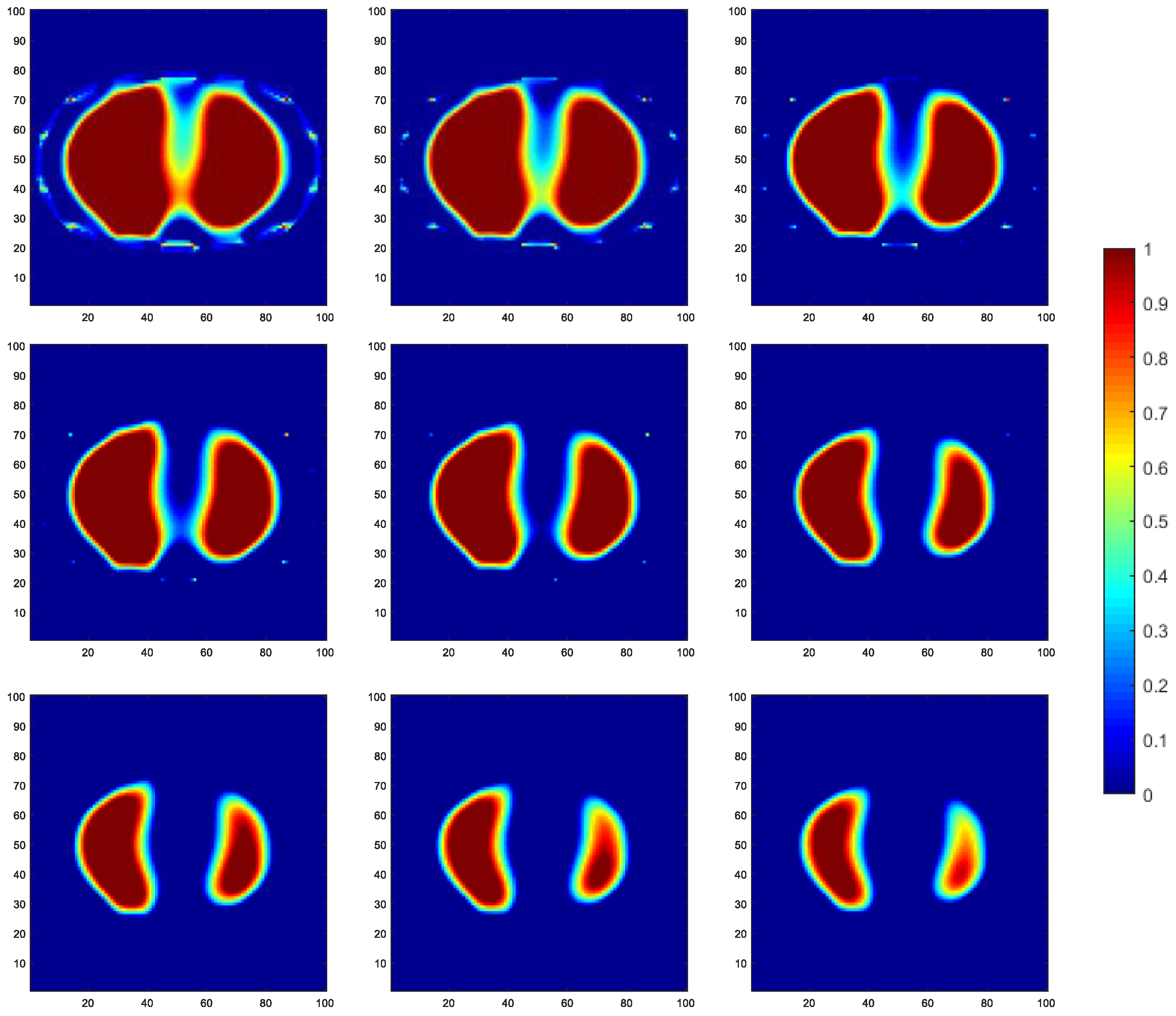
Using COMSOL Multiphysics 5.6 software, the boundary impedance data were obtained. By employing the Tikhonov regularization algorithm, reconstructed images of the tested field were obtained. These reconstructed images were then used as the original objects for segmentation. As an example, with a relaxation factor of 0.2, the segmentation threshold within the grayscale range was iterated with a fixed step size. The segmentation process for the original image is illustrated in Figure 3.
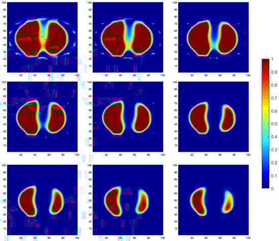
Figure 3.
Region segmentation process with a relaxation factor of 0.2.
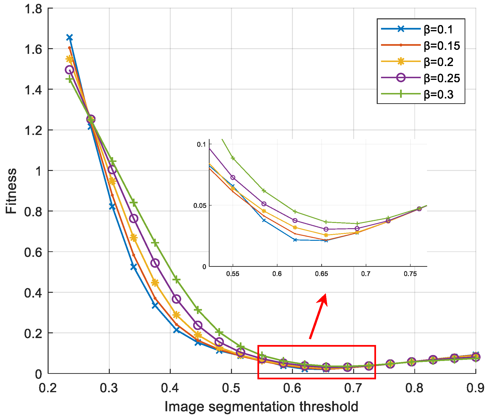
Based on the desired segmentation result as the basis for the relaxation factor input, in this case, it is only necessary to optimize the objective functional construction based on the one-dimensional variable of the segmentation threshold according to the previous text. In the process of parameter optimization, this paper refers to the image processing method for deformation cell tracking described in reference [29]. Therefore, the computational complexity of the soft-threshold region segmentation algorithm is smaller compared to the maximum entropy threshold segmentation method. The fitness change curve of the search process for the most suitable segmentation threshold under different relaxation factors is shown in Figure 4.
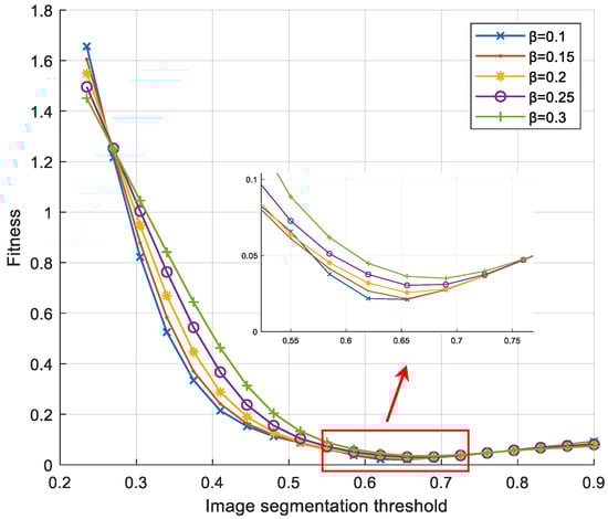
Figure 4.
Fitness curve of fitness against segmentation threshold under different relaxation factors.
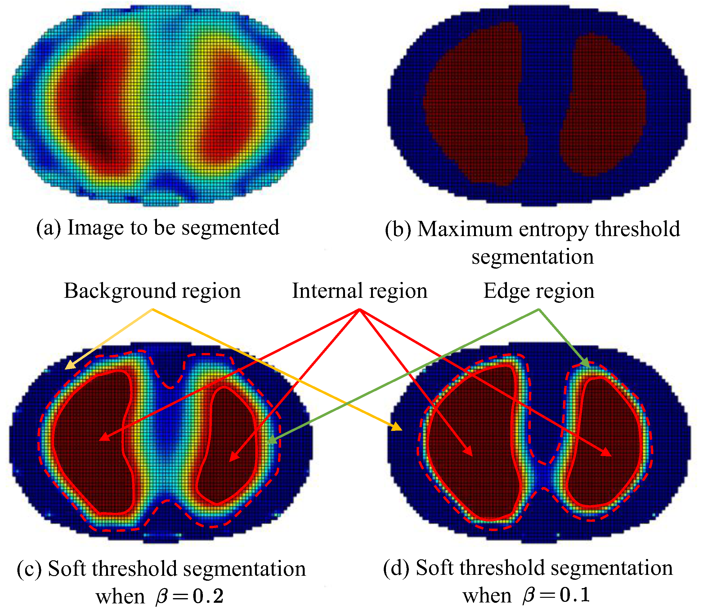
Using the reconstructed images obtained by the Tikhonov regularization algorithm as the original objects for segmentation, both the proposed soft-threshold region segmentation method and the maximum entropy threshold segmentation method were utilized for image segmentation. The relaxation factors for the soft-threshold region segmentation were set to 0.1 and 0.2, respectively. The comparison of segmentation results is shown in Figure 5.
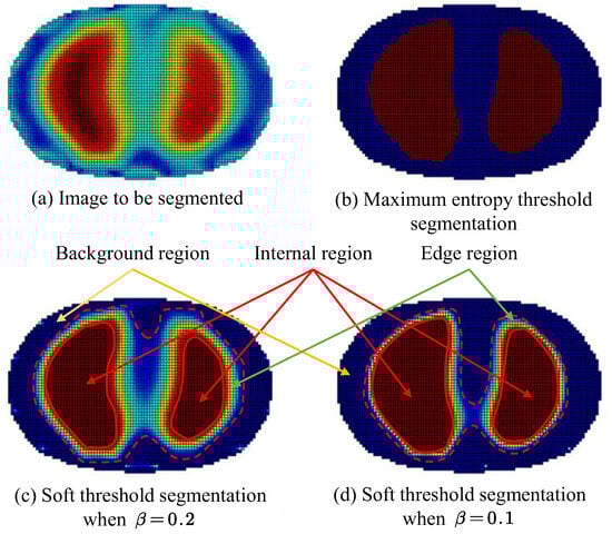
Figure 5.
Comparison of image segmentation results. (Red arrow points Internal region; Green arrow points Edge region; Yellow arrow points Background region).
From the visualization of the segmentation results shown in Figure 5, it can be observed that by inputting different relaxation factors, control over the extent of preservation of the edge region q2 can be achieved, thus meeting the segmentation requirements under different conditions. Furthermore, when the relaxation factor is set to a low value, the segmentation results of the target area obtained by the soft thresholding area segmentation method, that is, the dashed line portion in the figure, are similar to those obtained by the maximum entropy threshold segmentation method. In the figure mentioned above, the maximum entropy threshold segmentation method resulted in the target area retaining 1893 pixels. When the relaxation factor was set to 0.1, 2144 pixels were retained, and with a relaxation factor of 0.2, 2613 pixels were retained
In certain conditions that demand high accuracy in the segmentation results, where misclassification between the region of interest and the background can lead to severe consequences, a larger relaxation factor should be used to preserve the potential medium information at the segmentation boundary and ensure the accuracy of the segmentation results. Conversely, in other conditions where there is a higher requirement for the segmentation effect, such as the need for a clear contour boundary for the region of interest, but with relatively lower accuracy requirements, accepting a certain degree of misclassification between the region of interest and the background is acceptable. In such cases, a smaller relaxation factor should be used to mitigate potential reconstruction artifacts in the images, such as in the continuous detection of lung respiration states.
Compared to the maximum entropy segmentation algorithm, the proposed soft-threshold region segmentation algorithm with a relaxation factor not only reduces the computational complexity but also expands the applicability of segmentation algorithms in EIT problems. Moreover, this algorithm can be better matched with the subsequent reduced-order Tikhonov regularization algorithm mentioned in the following text, thereby improving the ill-posedness of EIT reconstruction problems.
4. Reduced-Order Tikhonov Regularization Imaging Based on Soft-Threshold Segmentation
During the process of electrical impedance tomography (EIT) image reconstruction, the number of image pixels is much larger than the number of boundary measurements. To obtain higher-quality reconstructed images, increasing the number of image pixels is necessary, which further increases the ill-posedness of the image reconstruction process. However, if the pixels belonging to the background region in the image are removed from the solution process, it can partially improve the ill-posedness of the problem-solving process. Moreover, removing more background regions while ensuring the preservation of the region of interest leads to a better improvement in image reconstruction.
The reduced-order Tikhonov algorithm considers grayscale value of 0 pixels in the reconstructed image as the background, which helps reduce the number of unknowns. In this study, based on the results of the image segmentation algorithm, the pixels belonging to the background region are removed from the solution process. This reduction in unknowns is done while maintaining the same number of equations in the inverse problem formulation. After solving for the pixel values in the region of interest, they are merged with the background region obtained through image segmentation to obtain a new reconstructed image. The specific steps are as follows:
- Firstly, an existing image reconstruction algorithm is used to obtain an initial distribution map g of the medium field, which serves as the initial image for subsequent image processing. The initial algorithm used in this study is the Tikhonov regularization algorithm.
- An image segmentation algorithm is used to segment the initial distribution map g into three parts: the inner region q1, the edge region q2, and the background region q3. The segmented medium distribution image is denoted as g*1.
- The background region is removed from the image reconstruction process to reduce the number of unknowns. The corresponding rows of the sensitivity matrix S are reduced based on the image segmentation result. The reduced sensitivity matrix is denoted as S*. The process of obtaining the reduced sensitivity matrix is shown as follows:
- Based on the obtained reduced sensitivity matrix S, the Tikhonov regularization imaging algorithm is applied to reconstruct the inner region q1 and the edge region q2. The reconstructed image after dimension reduction is denoted as .
- For the reconstructed image after dimension reduction, it is restored to the complete image based on the segmented medium distribution and the image segmentation result. The mathematical expression for the image restoration process is shown as follows:
- For the obtained complete reconstructed image , an image segmentation algorithm is applied once again to perform image segmentation and extract the regions of interest.
The algorithm flowchart is shown in Figure 6. Different relaxation factors should be selected for different application conditions. For obtaining the reduced-order Tikhonov regularization, a larger relaxation factor is used to preserve the medium information that may exist at the segmentation edges and ensure that the regions of interest, including the inner region q1 and the edge region q2, are not mistakenly eliminated when excluding the background region q3. In order to achieve a clearer representation of the regions of interest, a smaller relaxation factor is chosen to mitigate potential artifacts in the reconstructed image.
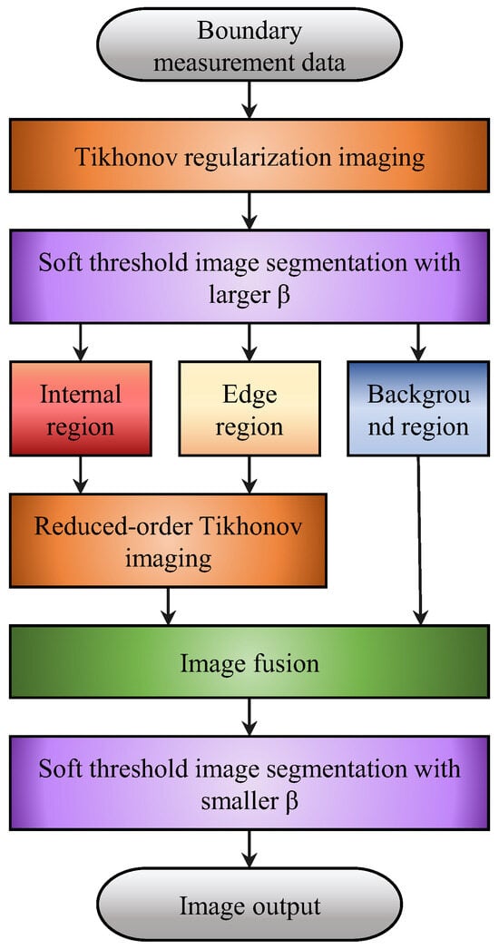
Figure 6.
Flowchart of the region segmentation-reduced-order Tikhonov regularization imaging algorithm.
Compared to the conventional reduced-order Tikhonov algorithm that treats pixels with a grayscale value of 0 in the original image as background and eliminates them, performing soft-threshold region segmentation on the original image before dimension reduction allows for the identification of a wider range of background areas while preserving the target regions. This effectively reduces the number of unknowns in the solution and improves the ill-posedness of the EIT image reconstruction process. Additionally, as an effective image post-processing approach, performing soft-threshold region segmentation on the reduced-order Tikhonov image produces reconstructed images with clearer boundary contours. This facilitates further parameter calculations and assists medical professionals in identification and judgment.
5. Numerical Simulation and Experimental Verification
5.1. Simulation Experimental Platform
To validate the stability and effectiveness of the proposed algorithm, a human lung model is established as the research object, and a 16-electrode EIT simulation model of the human thorax is constructed. The 16 measurement electrodes are uniformly distributed on the surface of the thorax, and the forward problem is solved using the COMSOL Multiphysics 5.6 software, resulting in 2993 mesh elements, as shown in Figure 7. Based on the established model, 120 sets of valid boundary impedance data can be obtained for a specific lung condition using the 16 measurement electrodes. These data are input into MATLAB software to achieve image reconstruction. The reconstructed image is then compared with the ground truth image to quantitatively evaluate the imaging performance. The simulations in this study were conducted on a PC equipped with an Intel Core 2 E8200 2.66 GHz CPU (Intel Corporation, Santa Clara, CA, USA), and 8 GB of RAM. This configuration meets the computational cost requirements for simulations in COMSOL Multiphysics 5.6.
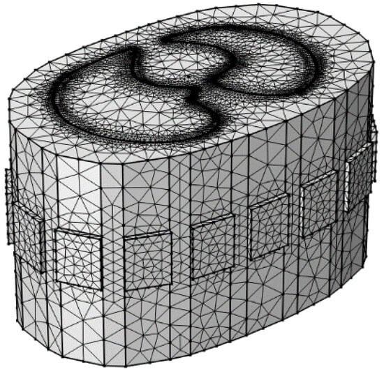
Figure 7.
A three-dimensional finite element model of the human thoracic field with 16-electrode configuration.
5.2. Image Evaluation Metrics
- (1)
- Relative Error of Reconstructed Images (IRE)
The fidelity of the reconstructed image compared to the ground truth image is a crucial evaluation criterion for image reconstruction. The relative error of the reconstructed image (IRE) captures the errors between the reconstructed image and the ground truth image in terms of shape, area, and other aspects, effectively reflecting the differences between the two. The calculation formula for IRE is given as follows.
In the above equation, g represents the reconstructed medium distribution obtained through the imaging reconstruction algorithm, and g0 represents the actual medium distribution in the field in the simulation experiment. A smaller value of the relative error indicates a higher image quality.
- (2)
- Image Correlation Coefficient (ICC)
The image correlation coefficient is an important metric for evaluating the degree of correlation between the reconstructed image and the ground truth image. It represents the correlation between the actual distribution and the reconstructed image. The calculation formula for the image correlation coefficient is given as follows.
In the above equation, g′ represents the mean value of the reconstructed image’s medium distribution, g0′ represents the mean value of the medium distribution in the region of interest in the ground truth image, and n represents the number of pixels in the image.
- (3)
- Structural Similarity Index (SSIM)
SSIM is a metric for measuring the similarity between two images in terms of their structure. It is introduced as a standard to evaluate the similarity between the reconstructed image and the ground truth image. The calculation formula for SSIM is given as follows.
In the above equation, ux and represent the mean and variance of the reconstructed image, while uy and represent the mean and variance of the ground truth image. σxy represents the covariance between the reconstructed image and the ground truth image. c1 and c2 are constants, usually set to very small values to avoid division by zero. A larger value of SSIM indicates a higher structural similarity between the two images and a better result in the image reconstruction.
5.3. Numerical Simulation Verification
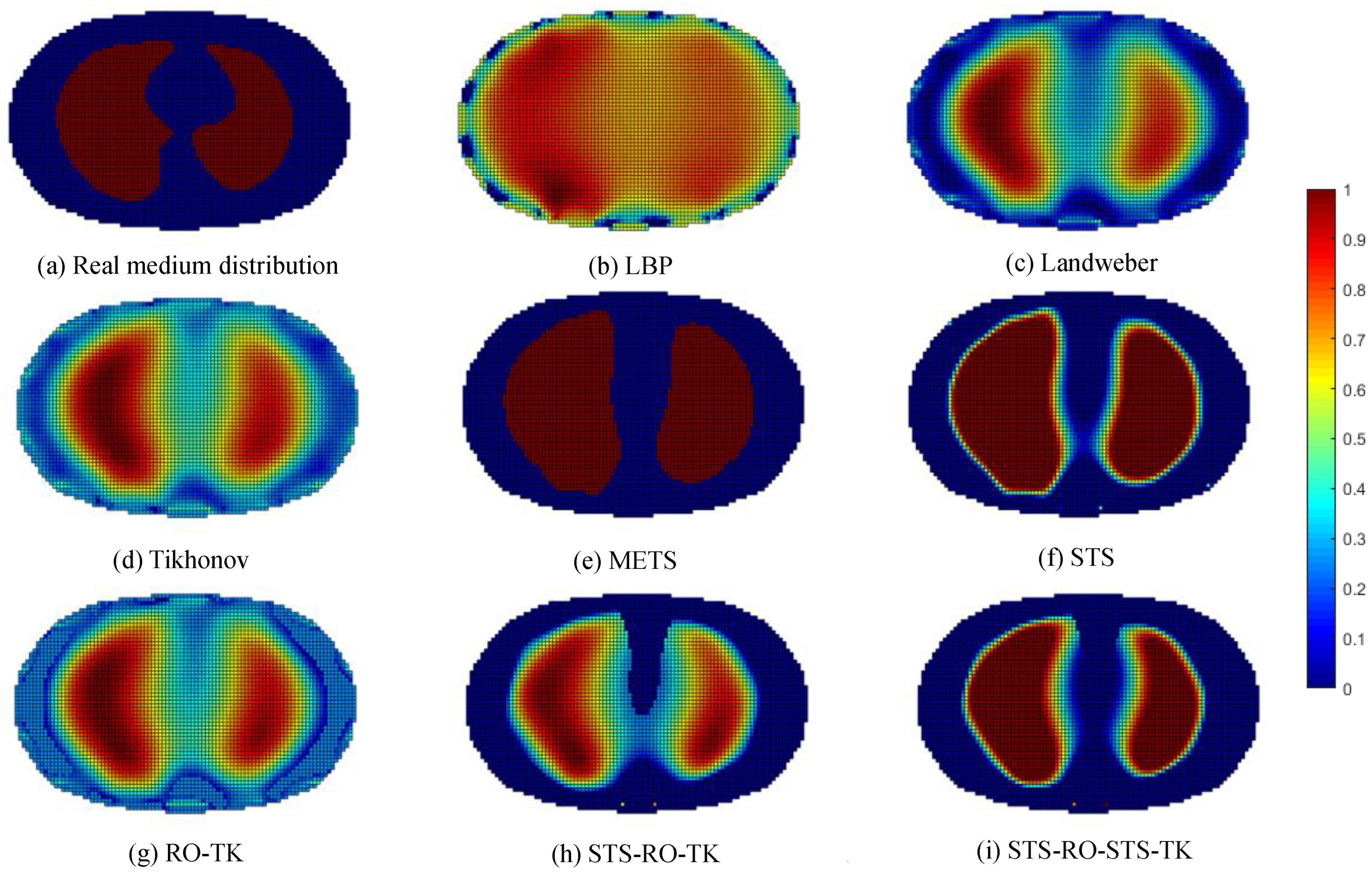
To validate the effectiveness of the soft-threshold region segmentation algorithm and its compatibility with the reduced-order Tikhonov regularization algorithm, a 16-electrode EIT simulation model of the human thoracic field was established. Numerical simulations were conducted using commonly used image reconstruction algorithms, including the local binary patterns (LBP) algorithm, the Landweber algorithm, and the classical Tikhonov regularization algorithm. A comparative analysis of the imaging results was performed using the maximum entropy threshold segmentation algorithm (METS) and a single reduced-order Tikhonov regularization algorithm (RO-TK). Numerical simulations were also conducted for the METS, soft-threshold segmentation algorithm (STS), reduced-order Tikhonov regularization algorithm (RO-TK), segmentation-reduced-order Tikhonov regularization algorithm (STS-RO-TK), and segmentation-reduced-order-segmentation Tikhonov regularization algorithm (STS-RO-STS-TK). The relationship between the abbreviations and the full names of the algorithms involved in this paper can be found in Table A1 in Appendix A. The initial images for the METS and STS algorithms were obtained using the reconstruction images from the Tikhonov regularization algorithm. The resulting comparative images of the various algorithms for image reconstruction are shown in Figure 8.
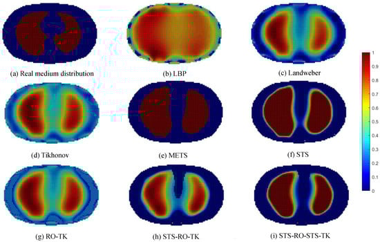
Figure 8.
Comparative reconstructed images of various algorithms based on simulated data.
By observing the image reconstruction results, it can be noticed that the LBP algorithm only approximates the imaging target, and the image boundaries are very blurry. Moreover, its performance in reconstructing the left and right lung images is poor. The Landweber algorithm and the Tikhonov algorithm are able to reconstruct the left and right lung regions more distinctly, but the image boundaries are not sharp enough. Using self-used threshold segmentation or maximum entropy threshold segmentation algorithms can clearly define the boundary of the region of interest, but the reconstructed image shapes deviate from the real distribution. In contrast, the reconstructed image obtained using the reduced-order Tikhonov regularization can better depict the details of the image boundaries compared to traditional Tikhonov regularization, resulting in a closer representation of the actual medium distribution. Furthermore, applying soft-threshold region segmentation on the reconstructed image obtained using reduced-order Tikhonov regularization can reduce image artifacts within the internal region and further clarify the lung regions of interest.
Evaluation of image reconstruction results for various imaging algorithms discussed in this paper was conducted using the image evaluation metric calculation method provided in the previous section. The results of the evaluation metrics for the image reconstruction results obtained based on measurements from the simulation model are shown in Table 1 and Figure 9.

Table 1.
Comparative evaluation of reconstructed image metrics based on simulated data for various algorithms.
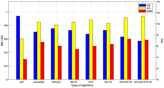
Figure 9.
Comparative evaluation of various algorithm metrics based on simulated data.
The analysis of the image evaluation metrics leads to the following conclusions: the use of image segmentation algorithms can reduce the relative error (IRE) of the reconstructed images and improve the image correlation coefficient (ICC). However, it may result in a certain degree of decrease in the structural similarity index (SSIM) of the images. In particular, the proposed soft-threshold segmentation method in this study achieves a more significant improvement in ICC and a reduction in IRE with a lesser loss in SSIM compared to the maximum entropy threshold segmentation method. The reduced-order Tikhonov algorithm can effectively enhance the SSIM and to some extent improve the ICC and reduce the IRE, although its improvement is not as significant as that achieved by using image segmentation algorithms. The proposed segmentation-reduced-order-Tikhonov algorithm (STS-RO-TK) can leverage the advantages of both algorithms, effectively maintaining a high SSIM while reducing IRE and improving ICC.
From the perspective of alleviating the ill-posedness of the image reconstruction process, the fewer unknowns solved during the inverse problem-solving process, the less severe the ill-posedness. In this study, the images of the internal medium distribution within the reconstructed field were obtained at a resolution of 100 × 100 pixels. Compared to the original reduced-order Tikhonov algorithm (RO-TK) regularization algorithm, which reduces 701 unknowns, the proposed segmentation-reduced-order-Tikhonov algorithm (STS-RO-TK) can reduce 2169 unknowns, thus improving the ill-posedness of the image reconstruction process. For further refinement of the reconstructed images, the segmentation-reduced-order-segmentation-Tikhonov regularization algorithm (STS-RO-STS-TK) can be applied after the segmentation-reduced-order-Tikhonov (STS-RO-TK) reconstruction to obtain images with even clearer boundaries.
6. Experimental Validation
6.1. Experimental Platform Setup
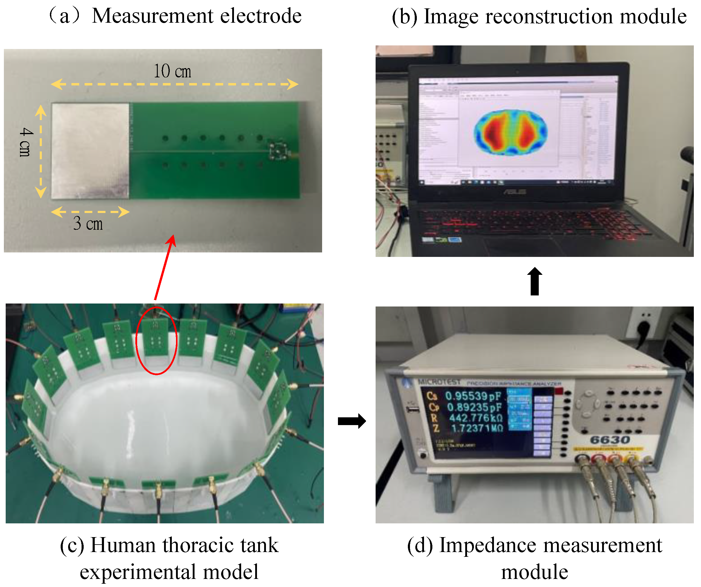
We constructed a human thoracic impedance tomography (EIT) experimental platform, which includes a human thoracic tank experimental model, an impedance measurement module, and an image reconstruction module. The thoracic tank experimental model consists of 16 array measurement electrodes, which are arranged in a uniform polar distribution along the edges of the tank experimental model. During the experiment, a gelatin gel prepared by mixing gelatin powder and distilled water is used to simulate the human lung region. A sodium chloride solution is used to simulate the peripheral region of the chest. The impedance measurement module utilizes a Yehoch 6630 precision impedance analyzer to measure the boundary impedance signals between different electrodes at a frequency of 500 kHz. The measurement electrodes are made of specification-controlled PCD boards, which facilitate installation and removal. The effective measurement area is 3 cm × 4 cm, and the electrodes are made of tin-plated metal materials. SMA-shielded cables are used to connect the measurement electrodes with the impedance analyzer to effectively avoid interference from stray signals. The image reconstruction module consists of a PC with an Intel Core 2 E8200 2.66 GHz CPU and 16 GB of memory. Image reconstruction is implemented using MATLAB software. The schematic diagram of the constructed experimental platform is shown in Figure 10.
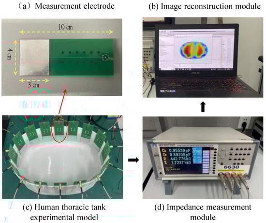
Figure 10.
Schematic diagram of the experimental setup for human thoracic impedance tomography.
6.2. Analysis of Experimental Results
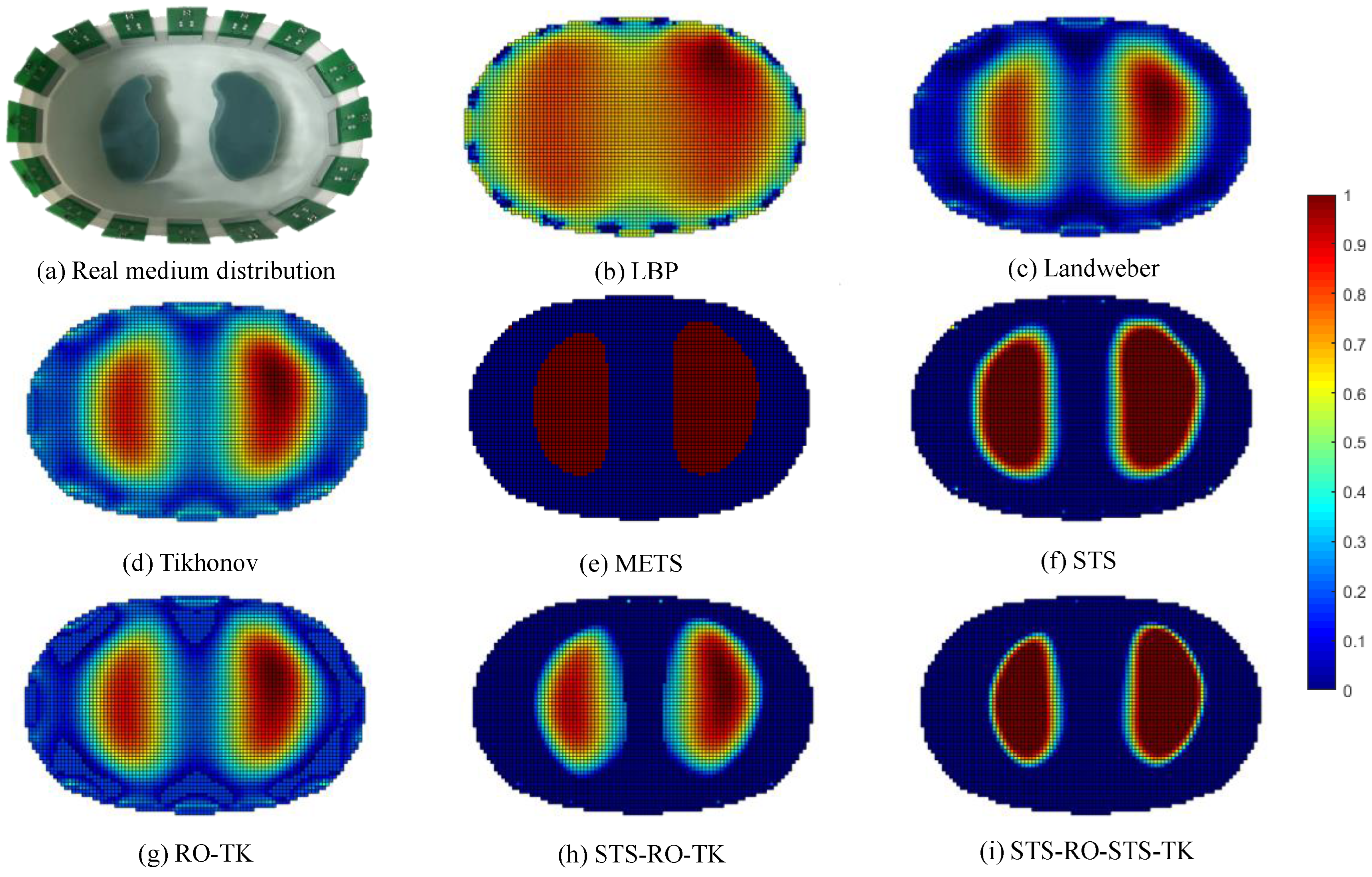
Based on the experimental platform of human lung impedance tomography, the boundary electrode impedance measurement signals were acquired and fed into a PC. Image reconstruction was then conducted using various programmed imaging algorithms in MATLAB software. The resulting reconstructed image is shown in Figure 11.
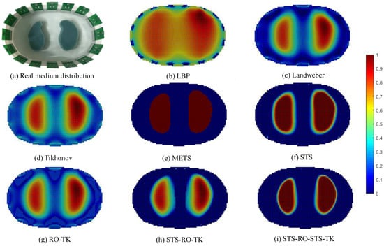
Figure 11.
Comparative images of various algorithms for image reconstruction based on experimental data.
Evaluation of the image reconstruction results for various imaging algorithms discussed in this paper was performed using the image evaluation metric calculation method mentioned earlier. The evaluation metrics for the image reconstruction results, which were obtained based on experimental measurements, are presented in Table 2 and Figure 12.
Table 2.
Comparative table of image evaluation metrics for various algorithms for image reconstruction based on experimental data.
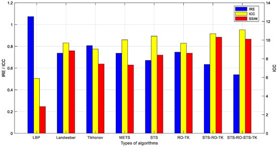
Figure 12.
Comparative evaluation of various algorithm metrics based on experimental data.
By visually observing the EIT reconstructed images based on experimental measurement data, it can be observed that they exhibit certain similarities with the EIT reconstructed images based on simulated data in terms of overall effects. However, due to the influence of contact impedance and noise signals, the reconstructed images based on experimental data exhibit less detail compared to the simulated reconstructed images, and certain distortions can be observed in some areas. Nevertheless, when comparing different imaging algorithms under the condition of experimental measurement data, it is found that the proposed soft-threshold segmentation method (STS) can effectively identify the pulmonary region of interest in the thoracic cavity. Combining the soft-threshold segmentation method (STS) with the reduced-order Tikhonov algorithm (RO-TK) and utilizing the segmentation-reduced-order-segmentation Tikhonov algorithm (STS-RO-STS-TK), the reconstructed images demonstrate a closer resemblance to the test model in terms of the reconstructed target shape. Furthermore, by calculating the evaluation metrics of the reconstructed images, it is found that the reduced-order Tikhonov algorithm (RO-TK) with image segmentation processing yields superior evaluation metrics compared to the standalone reduced-order Tikhonov algorithm (RO-TK). This further validates the effectiveness of the proposed method.
7. Conclusions
Electrical impedance tomography (EIT) often yields low-quality reconstructed images due to the inherent ill-posedness of the inverse problem. In this paper, image segmentation techniques are introduced into EIT imaging, and a soft-threshold image segmentation method with a relaxation factor is proposed. The original image is segmented into three regions: the internal region, the edge region, and the background region. The selection of segmentation thresholds is based on optimizing the error norm between the boundary values of the segmented image and the true measured boundary impedance. By adjusting the relaxation factor, the degree of preservation of the edge region can be controlled. This segmentation method is used for the post-processing of lung reconstruction images in EIT. Furthermore, this soft-threshold image segmentation method effectively combines with the reduced-order Tikhonov algorithm by removing the discretization points belonging to the background region from the sought grayscale vector, thereby improving the ill-posedness issue in EIT. The main conclusions of this study are the following:
- Post-processing of lung EIT reconstruction images using image segmentation algorithms allows for effective identification of regions of interest, resulting in clear and distinguishable human lung images with well-defined edges. However, this process may lead to some information loss. In terms of evaluation metrics, the use of image segmentation algorithms reduces the relative error (IRE) and improves the image correlation coefficient (ICC) of the reconstructed images, but it may decrease the structural similarity index (SSIM).
- Compared to fixed threshold segmentation methods, such as the maximum entropy threshold segmentation method, soft-threshold segmentation allows for adjusting the preservation degree of the edge region connected to the regions of interest and the background region. This widens the application scope of segmentation algorithms for EIT reconstruction by catering to different processing requirements.
- The reduced-order Tikhonov algorithm addresses the ill-posedness issue in EIT by excluding the partition points belonging to the background region from the sought grayscale vector. The combination of image segmentation algorithms and the reduced-order Tikhonov algorithm effectively enhances the ill-posedness issue in image reconstruction, resulting in higher-quality reconstructed images.
Finally, the effectiveness of the proposed algorithms was further demonstrated through numerical simulations and experimental verification using a 16-electrode human thoracic EIT simulation model and a human thoracic impedance tomography experimental platform.
In summary, this paper introduces image segmentation algorithms into human lung electrical impedance tomography (EIT) technology, enabling the reconstruction of images that are closer to the real cross-sectional images of human lungs. Furthermore, these images facilitate easier recognition of lung contours by individuals.
Author Contributions
Conceptualization, Y.S. and L.X.; methodology, Y.S. and Z.L.; software, Y.S.; validation, Y.S., L.X., and Z.L.; formal analysis, Y.S. and Y.W.; investigation, Y.S. and Y.W.; resources, Z.Z.; data curation, Z.Z.; writing—original draft preparation, Y.S.; writing—review and editing, Z.Z.; visualization, L.X.; supervision, Z.Z.; project administration, Z.Z.; funding acquisition, Z.Z. All authors have read and agreed to the published version of the manuscript.
Funding
This research received no external funding.
Institutional Review Board Statement
Not applicable.
Informed Consent Statement
Not applicable.
Data Availability Statement
Data associated with this research are available and can be obtained by contacting the corresponding author upon reasonable request.
Conflicts of Interest
Author Yongye Wu was employed by the company Chengdu Power Supply Company, State Grid Sichuan Electric Power Company. The remaining authors declare that the research was conducted in the absence of any commercial or financial relationships that could be construed as a potential conflict of interest.
Appendix A
Table A1.
The table provided in the text corresponds to a list of algorithm abbreviations and their full names as used within the document:
Table A1.
The table provided in the text corresponds to a list of algorithm abbreviations and their full names as used within the document:
| Serial No. | Abbreviation | Full Name of the Algorithm |
|---|---|---|
| 1 | LBP | Linear back projection algorithm |
| 2 | Landweber | Landweber iterative imaging algorithm |
| 3 | Tikhonov | Tikhonov regularization algorithm |
| 4 | METS | Maximum entropy threshold segmentation algorithm |
| 5 | STS | Soft-threshold segmentation algorithm |
| 6 | RO-TK | Reduced-order Tikhonov regularization algorithm |
| 7 | STS-RO-TK | Segmentation-reduced-order Tikhonov regularization algorithm |
| 8 | STS-RO-STS-TK | Segmentation-reduced-order-segmentation Tikhonov regularization algorithm |
References
- Krick, S.; Geraghty, P.; Jourdan Le Saux, C.; Rojas, M.; Staab-Weijnitz, C.A. Defining and Characterizing Respiratory Disease in an Aging Population. Front. Med. 2022, 9, 889834. [Google Scholar] [CrossRef] [PubMed]
- Zhang, Y.; Wang, Z.; Cao, Y.; Zhang, L.; Wang, G.; Dong, F.; Deng, R.; Guo, B.; Zeng, L.; Wang, P.; et al. The Effect of Consecutive Ambient Air Pollution on the Hospital Admission from Chronic Obstructive Pulmonary Disease in the Chengdu Region, China. Air Qual. Atmos. Health 2021, 14, 1049–1061. [Google Scholar] [CrossRef] [PubMed]
- Shono, A.; Kotani, T.; Frerichs, I. Personalisation of Therapies in COVID-19 Associated Acute Respiratory Distress Syndrome, Using Electrical Impedance Tomography. J. Crit. Care Med. 2021, 7, 62–66. [Google Scholar] [CrossRef] [PubMed]
- Nakamura, H.; Hirai, T.; Kurosawa, H.; Hamada, K.; Matsunaga, K.; Shimizu, K.; Konno, S.; Muro, S.; Fukunaga, K.; Nakano, Y.; et al. Current Advances in Pulmonary Functional Imaging. Respir. Investig. 2024, 62, 49–65. [Google Scholar] [CrossRef] [PubMed]
- Shono, A.; Kotani, T. Clinical Implication of Monitoring Regional Ventilation Using Electrical Impedance Tomography. J. Intensive Care 2019, 7, 4. [Google Scholar] [CrossRef] [PubMed]
- Piraino, T. An Introduction to the Clinical Application and Interpretation of Electrical Impedance Tomography. Respir. Care 2022, 67, 721–729. [Google Scholar] [CrossRef] [PubMed]
- Sbarbaro, D.; Vauhkonen, M.; Johansen, T.A. State Estimation and Inverse Problems in Electrical Impedance Tomography: Observability, Convergence and Regularization. Inverse Probl. 2015, 31, 045004. [Google Scholar] [CrossRef]
- Ding, M.; Li, X.; Zhao, S. Application of Constrained Coefficient Fuzzy Linear Programming in Medical Electrical Impedance Tomography. Appl. Math. Sci. Eng. 2022, 30, 762–776. [Google Scholar] [CrossRef]
- Yan, H.; Wang, Y.; Wang, Y.; Zhou, Y. An ECT Image Reconstruction Algorithm Based on Object-and-Background Adaptive Regularization. Meas. Sci. Technol. 2021, 32, 015402. [Google Scholar] [CrossRef]
- Ko, Y.F.; Cheng, K.S. U-Net-Based Approach for Automatic Lung Segmentation in Electrical Impedance Tomography. Physiol. Meas. 2021, 42, 025002. [Google Scholar] [CrossRef]
- Song, X.; Xu, Y.; Dong, F. Linearized Image Reconstruction Method for Ultrasound Modulated Electrical Impedance Tomography Based on Power Density Distribution. Meas. Sci. Technol. 2017, 28, 045404. [Google Scholar] [CrossRef]
- Wang, J. A Two-step Accelerated Landweber-type Iteration Regularization Algorithm for Sparse Reconstruction of Electrical Impedance Tomography. Math. Methods Appl. Sci. 2021, 47, 3261–3272. [Google Scholar] [CrossRef]
- Wang, Z.; Liu, X. A Regularization Structure Based on Novel Iterative Penalty Term for Electrical Impedance Tomography. Measurement 2023, 209, 112472. [Google Scholar] [CrossRef]
- Xu, Y.; Pei, Y.; Dong, F. An Adaptive Tikhonov Regularization Parameter Choice Method for Electrical Resistance Tomography. Flow. Meas. Instrum. 2016, 50, 1–12. [Google Scholar] [CrossRef]
- Shi, Y.; Zhang, Y.; Wang, M.; Lou, Y.; Zheng, S. Reconstruction of Conductivity Distribution Variation with Tikhonov and Wavelet Frame Combined Method for Electrical Impedance Tomography. Trans. Inst. Meas. Control 2023, 45, 2658–2668. [Google Scholar] [CrossRef]
- Liu, S.; Cao, R.; Huang, Y.; Ouypornkochagorn, T.; Ji, J. Time Sequence Learning for Electrical Impedance Tomography Using Bayesian Spatiotemporal Priors. IEEE Trans. Instrum. Meas. 2020, 69, 6045–6057. [Google Scholar] [CrossRef]
- Chen, B.; Abascal, J.; Soleimani, M. Electrical Resistance Tomography for Visualization of Moving Objects Using a Spatiotemporal Total Variation Regularization Algorithm. Sensors 2018, 18, 1704. [Google Scholar] [CrossRef] [PubMed]
- Song, Y.; Wang, Y.; Liu, D. A Nonlinear Weighted Anisotropic Total Variation Regularization for Electrical Impedance Tomography. IEEE Trans. Instrum. Meas. 2022, 71, 1–13. [Google Scholar] [CrossRef]
- Gong, B.; Schullcke, B.; Krueger-Ziolek, S.; Zhang, F.; Mueller-Lisse, U.; Moeller, K. Higher Order Total Variation Regularization for EIT Reconstruction. Med. Biol. Eng. Comput. 2018, 56, 1367–1378. [Google Scholar] [CrossRef]
- Shi, Y.; Kong, X.; Wang, M.; Wu, Y.; Yang, L. A Non-Convex L1-Norm Penalty-Based Total Generalized Variation Model for Reconstruction of Conductivity Distribution. IEEE Sens. J. 2020, 20, 8137–8146. [Google Scholar] [CrossRef]
- Guo, Q.; Li, X.; Hou, B.; Mariethoz, G.; Ye, M.; Yang, W.; Liu, Z. A Novel Image Reconstruction Strategy for ECT: Combining Two Algorithms With a Graph Cut Method. IEEE Trans. Instrum. Meas. 2020, 69, 804–814. [Google Scholar] [CrossRef]
- Borgmann, S.; Linz, K.; Braun, C.; Dzierzawski, P.; Spassov, S.; Wenzel, C.; Schumann, S. Lung Area Estimation Using Functional Tidal Electrical Impedance Variation Images and Active Contouring. Physiol. Meas. 2022, 43, 075010. [Google Scholar] [CrossRef]
- Khambampati, A.K.; Liu, D.; Konki, S.K.; Kim, K.Y. An Automatic Detection of the ROI Using Otsu Thresholding in Nonlinear Difference EIT Imaging. IEEE Sens. J. 2018, 18, 5133–5142. [Google Scholar] [CrossRef]
- Arshad, S.H.; Murphy, E.K.; Halter, R.J. Automated Segmentation and Feature Extraction in Cardiac Electrical Impedance Tomography Images. In Progress in Biomedical Optics and Imaging, Proceedings of the Medical Imaging 2018: Biomedical Applications in Molecular, Structural, and Functional Imaging, Houston, TX, USA, 11–13 February 2018; Gimi, B., Krol, A., Eds.; SPIE: Bellingham, WA, USA, 2018; p. 61. [Google Scholar]
- Seo, J.K.; Lee, J.; Kim, S.W.; Zribi, H.; Woo, E.J. Frequency-difference electrical impedance tomography (fdEIT): Algorithm development and feasibility study. Physiol. Meas. 2008, 29, 929–944. [Google Scholar] [CrossRef] [PubMed]
- Gao, H.; Kang, W. Tikhonov Regularization Parameter Based on Augmented Lagrange Improves Photoacoustic Tomography. In Applications of Digital Image Processing XLIII; Tescher, A.G., Ebrahimi, T., Eds.; SPIE: Bellingham, WA, USA, 2020; p. 76. [Google Scholar]
- Zhu, P.; Ding, Y.; Gu, Y. Emery Particles Identification under Contour Extraction with Maximum Entropy Approaches. Int. J. Model. Identif. Control 2021, 38, 81. [Google Scholar] [CrossRef]
- Chandrasekar, K.S.; Geetha, P. Highly Efficient Neoteric Histogram–Entropy-based Rapid and Automatic Thresholding Method for Moving Vehicles and Pedestrians Detection. IET Image Process 2020, 14, 354–365. [Google Scholar] [CrossRef]
- Thapa, S.; Lukat, N.; Selhuber-Unkel, C.; Cherstvy, A.G.; Metzler, R. Transient superdiffusion of polydisperse vacuoles in highly motile amoeboid cells. J. Chem. Phys. 2019, 150, 144901. [Google Scholar] [CrossRef]


Disclaimer/Publisher’s Note: The statements, opinions and data contained in all publications are solely those of the individual author(s) and contributor(s) and not of MDPI and/or the editor(s). MDPI and/or the editor(s) disclaim responsibility for any injury to people or property resulting from any ideas, methods, instructions or products referred to in the content. |
© 2024 by the authors. Licensee MDPI, Basel, Switzerland. This article is an open access article distributed under the terms and conditions of the Creative Commons Attribution (CC BY) license (https://creativecommons.org/licenses/by/4.0/).