RDD-YOLO: Road Damage Detection Algorithm Based on Improved You Only Look Once Version 8

Abstract

The detection of road damage is highly important for traffic safety and road maintenance. Conventional detection approaches frequently require significant time and expenditure, the accuracy of detection cannot be guaranteed, and they are prone to misdetection or omission problems. Therefore, this paper introduces an enhanced version of the You Only Look Once version 8 (YOLOv8) road damage detection algorithm called RDD-YOLO. First, the simple attention mechanism (SimAM) is integrated into the backbone, which successfully improves the model’s focus on crucial details within the input image, enabling the model to capture features of road damage more accurately, thus enhancing the model’s precision. Second, the neck structure is optimized by replacing traditional convolution modules with GhostConv. This reduces redundant information, lowers the number of parameters, and decreases computational complexity while maintaining the model’s excellent performance in damage recognition. Last, the upsampling algorithm in the neck is improved by replacing the nearest interpolation with more accurate bilinear interpolation. This enhances the model’s capacity to maintain visual details, providing clearer and more accurate outputs for road damage detection tasks. Experimental findings on the RDD2022 dataset show that the proposed RDD-YOLO model achieves an mAP50 and mAP50-95 of 62.5% and 36.4% on the validation set, respectively. Compared to baseline, this represents an improvement of 2.5% and 5.2%. The F1 score on the test set reaches 69.6%, a 2.8% improvement over the baseline. The proposed method can accurately locate and detect road damage, save labor and material resources, and offer guidance for the assessment and upkeep of road damage.

1. Introduction

Roads constitute the backbone of transportation and are a crucial component of urban and rural infrastructure. Well-maintained road infrastructure is a prerequisite for urbanization and economic development. Given the ongoing development in road construction in China, the scale and complexity of the road network have experienced explosive growth. As of the end of 2022, the total road mileage in China has reached 5.35 million kilometers, growing by 1.12 million km in the past decade. Among them, the mileage of highways has reached 177,000 km, ranking first globally [1]. However, as the scale of roads expands, road damage issues become increasingly prominent. Due to differences in vehicle loads and construction lifespans, these roads face varying degrees of damage. Road damages such as potholes and cracks not only affect the efficiency of road traffic but also increase the instability of vehicle travel, raising the probability of traffic accidents and posing a threat to the safety of vehicles and passengers. Therefore, to maintain road infrastructure and improve road safety, it is crucial to detect and repair these road damages in a timely manner, which places strict requirements on the task of road damage detection.

Although the currently proposed deep learning-based object detection techniques have demonstrated remarkable success, there still remain challenges and room for enhancement in the field of road damage detection. Firstly, road damage exhibits diverse types with irregular shapes and sizes, making the detection task inherently challenging. Secondly, road background images encompass various elements such as different road surface textures, vehicles, pedestrians, and buildings, which may interfere with the accurate detection of road damage and impact the model’s precision. Furthermore, the appearance of road damage varies under different lighting and weather conditions, adding complexity to the road damage detection task. To tackle these obstacles and improve the accuracy and robustness of detection, this paper improves the state-of-the-art (SOTA) YOLOv8 model and applies it to road damage detection, resulting in improved precision and performance. The main contributions of this paper are as follows:

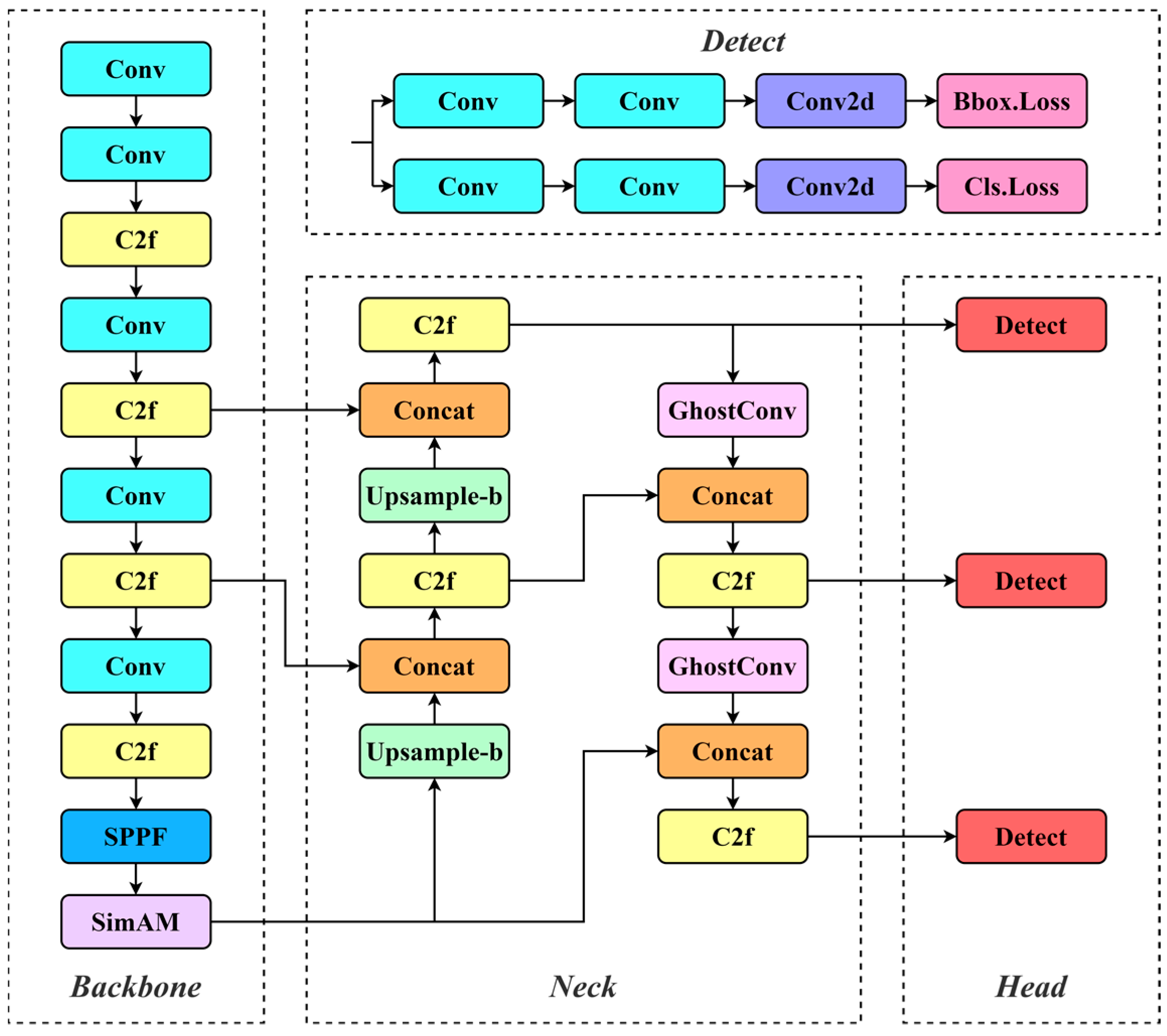
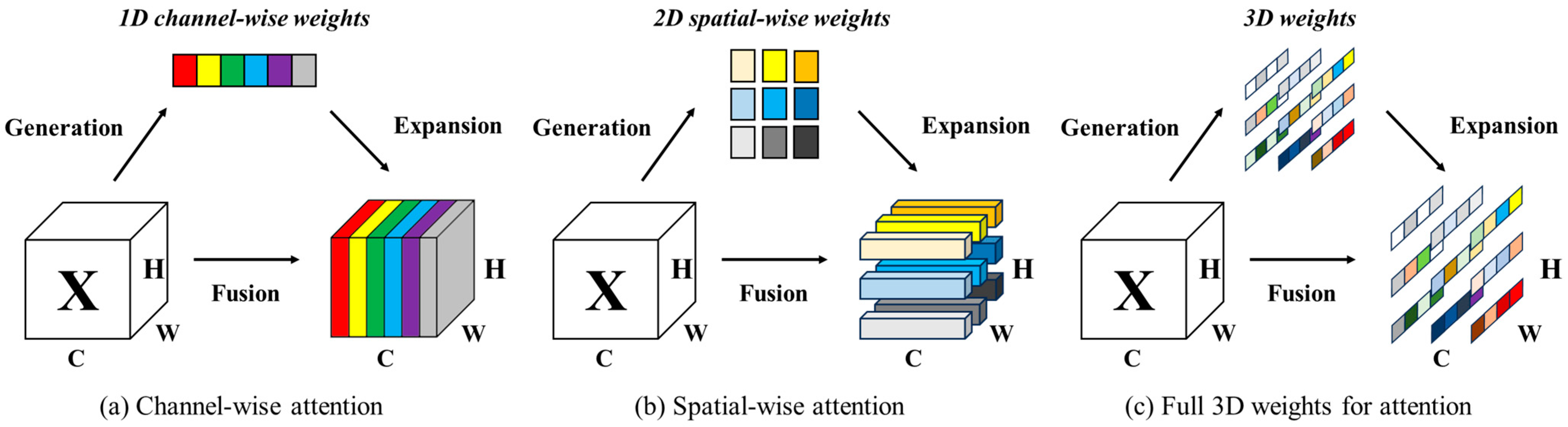
• The introduction of the SimAM [2] into the backbone filters out noise and amplifies the model’s focus on important information within the input image. This enhancement significantly improves the model’s performance and generalization ability, enhancing its ability to effectively handle road damage detection tasks.
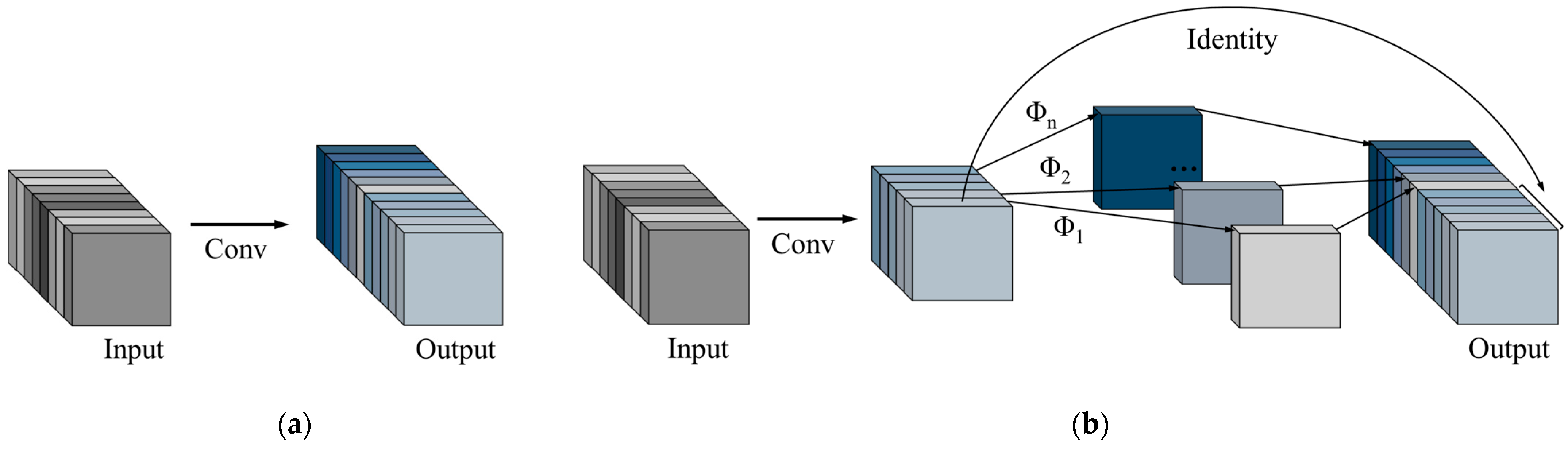
• The neck structure is enhanced by replacing traditional convolution modules with GhostConv [3]. This not only successfully reduces redundant information in the model, lowering the number of parameters and computational complexity, but also maintains the model’s outstanding performance in recognizing damage.
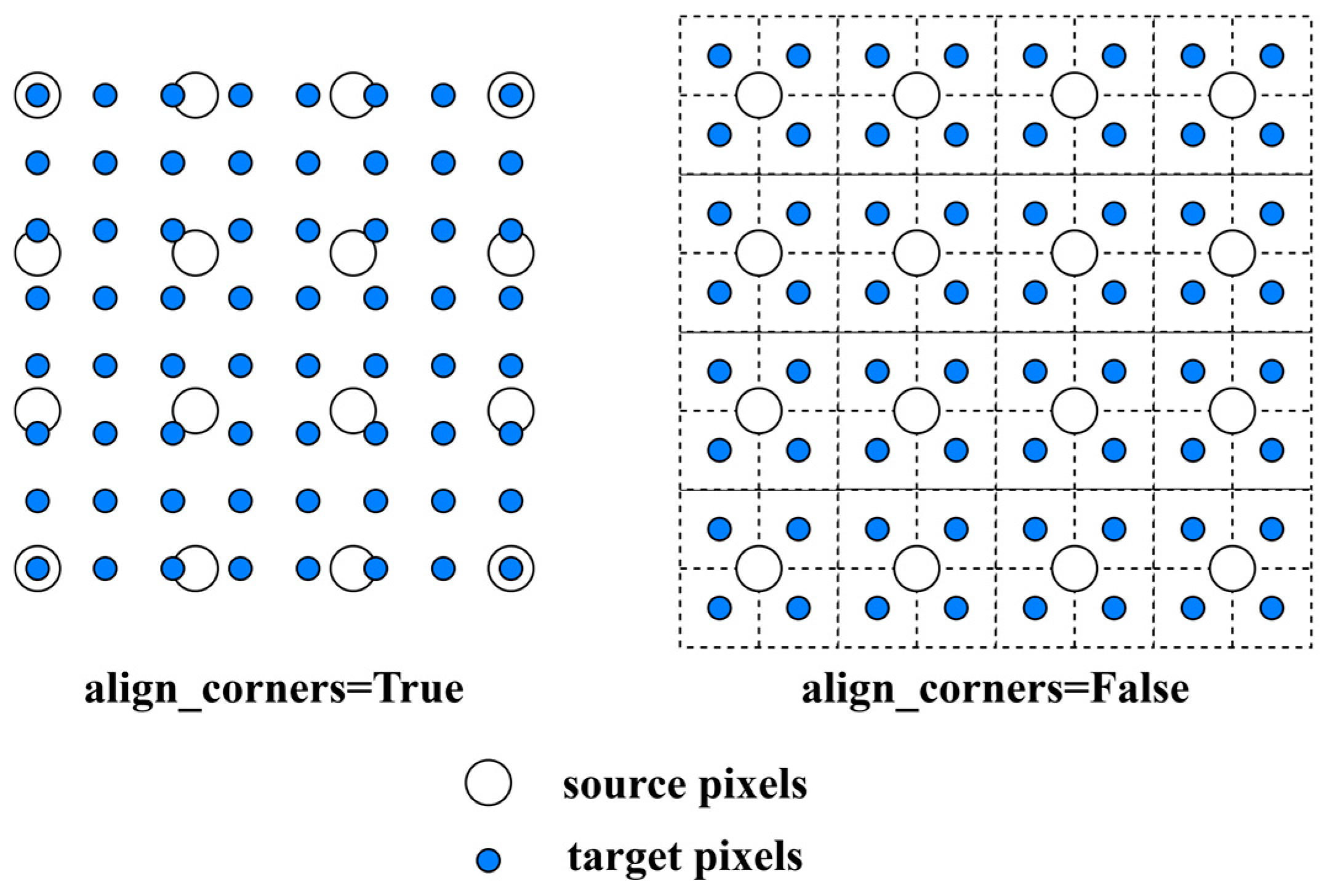
• To ensure the provision of more accurate images, the nearest interpolation in the neck is replaced with a more accurate bilinear interpolation. This modification enhances the model’s capability to retain complex details in the image, producing a clearer, more accurate output that helps minimize the impact of environmental factors on detection results.

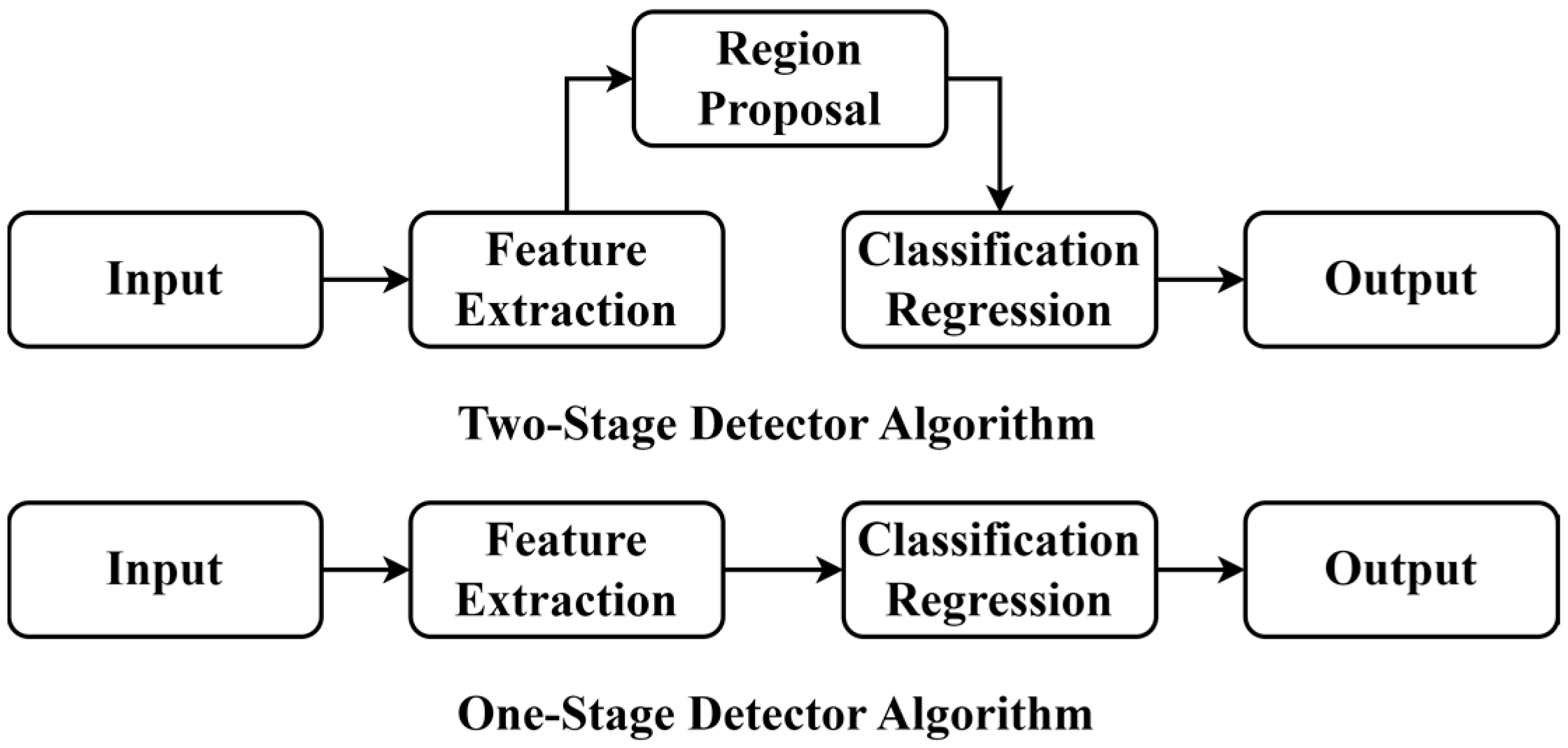
2. Related Work

2.1. Road Damage Detection

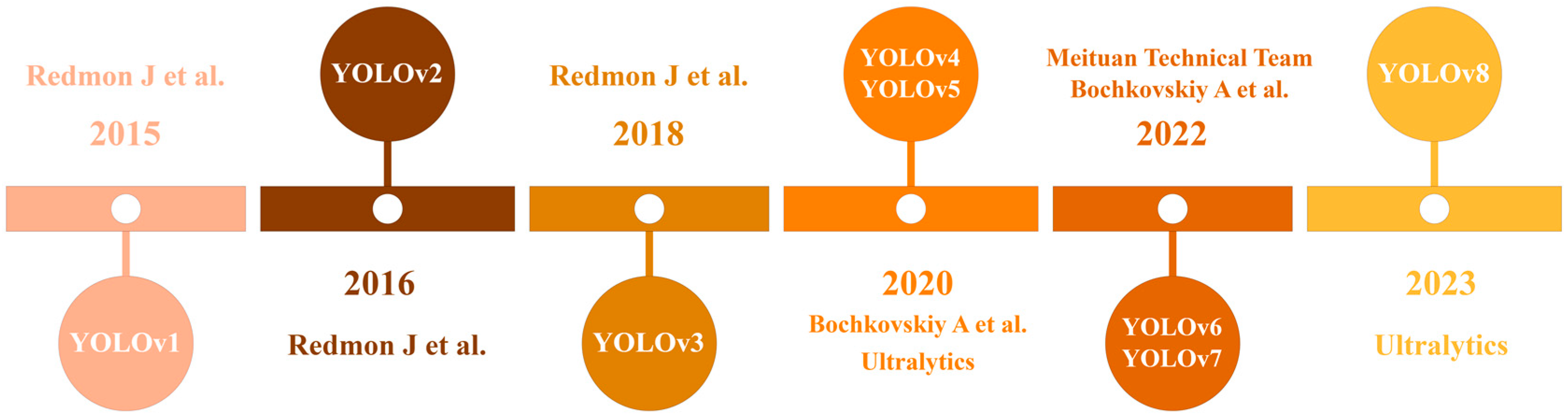
Conventional road damage detection approaches are mainly based on vehicle patrols, manual photography, and inspection personnel. This is laborious, inefficient, and often needs lots of manpower and resources. Additionally, during inspections, patrol vehicles and personnel often need to occupy the road, leading to potential traffic congestion and safety hazards. Moreover, manual detection heavily relies on the experience of inspection personnel and is subject to a certain degree of subjectivity. With the ongoing development of computer vision, image segmentation techniques based on manual feature extraction have emerged. These techniques can identify road damage by extracting characteristics such as edge information [4], histograms of oriented gradients [5], and wavelet transforms [6]. However, these methods often require manual design of feature extraction algorithms, have limited ability to capture semantic information, cannot fully utilize the rich features present in road damage images, exhibit poor generalization, and have limited effectiveness in complex scenarios.

Deep learning-based object detection algorithms offer a new solution to road damage detection. These methods can automatically identify the precise location, type, and boundary information of damages in images, enabling rapid and precise detection of road damage. Currently, many deep learning-based object detection algorithms have been utilized for road detection tasks. Fan Z et al. [7] proposed a convolutional neural network (CNN)-based supervised road surface crack detection technique, showing excellent performance in handling different road textures. Cao M T et al. [8] tested eight different road damage detection models based on Single Shot MultiBox Detector (SSD) and Faster Region–CNN(R-CNN), providing a performance comparison. Kang D et al. [9] created a method for detecting, localizing, and quantifying cracks by integrating Faster R-CNN, improved tubularity flow field (TuFF), and improved distance transform method (DTM) to detect crack areas, addressing practical issues with complex environmental backgrounds. Mandal V et al. [10] deployed SOTA deep learning algorithms based on different network backbones to detect and characterize pavement distresses. They investigated the impact of different backbone architectures including CSPDarknet53, Hourglass-104, and EfficientNet on the classification performance. Chen et al. [11] introduced a Mask R-CNN framework employing DenseNet as the feature map extraction backbone. They utilized a feature pyramid network to integrate features across multiple scales, a region proposal network for generating road damage regions, and a fully convolutional neural network to classify and refine region boundaries. This approach enables not only the detection and classification of road damage but also the creation of a mask of the road damage. Yuan Y et al. [12] introduced an innovative privacy-preserving edge cloud and federated learning-based framework named FedRD for intelligent detection and warning of hazardous road damage. This method provides inexpensive, quick, precise, and private road damage detection and warning. Zhang Y et al. [13] proposed a multi-level attention mechanism named Multi-level Attention Block (MLAB) to enhance the utilization of critical features by YOLOv3. The network can accurately detect longitudinal cracks, transverse cracks, repairs, and potholes and notably enhances the accuracy of detecting alligator cracks and oblique cracks. Wang J et al. [14] introduced an improved YOLOv5 road surface damage detection method, GSC-YOLOv5, enhancing the detection capability for small cracks and improving accuracy while reducing the model’s parameter count. Ni Y et al. [15] introduced a three-stage approach for bridge road damage and lane positioning based on YOLOv7 and improved LaneNet. This approach attained satisfactory outcomes in bridge road damage detection and lane positioning tasks.

2.2. YOLO Algorithm

The development of object detection can be classified into two directions: one-stage detection algorithms and two-stage detection algorithms. As illustrated in Figure 1, two-stage detection algorithms generate region proposals after feature extraction and are followed by classification and regression operations on the region proposals to produce results. In contrast, one-stage detection algorithms do not need to generate region proposals. They directly extract features in the network for classification and regression operations, producing results without an intermediate step. YOLO belongs to the one-stage object detection algorithm category. It transforms the object detection problem into an end-to-end regression problem, predicting all object bounding boxes and categories simultaneously using a single feed-forward neural network. It can detect and locate objects directly from the image in a single forward pass.

Figure 2 shows the evolution timeline of the YOLO algorithm. YOLOv1, the initial version of the YOLO algorithm, was introduced by Joseph Redmon et al. at the University of Washington in 2015 grid [16] and analyzes whether each border is the position and confidence of the detected object [17]. YOLOv1 has a small computational load and fast runtime, but it is less effective in detecting small targets and requires accuracy improvement. In 2017, Joseph Redmon et al. proposed YOLOv2 [18]. It incorporates batch normalization to improve model convergence, further accelerating training speed. YOLOv2 also introduces anchor boxes to improve the detection capabilities for objects of different sizes. Additionally, YOLOv2 can simultaneously detect over 9000 different classes, so it is also called YOLO9000, which is more versatile. In 2018, Joseph Redmon et al. released YOLOv3 [19], introducing residual networks, spatial pyramid pooling (SPP), and cross-stage partial networks (CSPNet) for multi-scale detection. YOLOv3 deepens the network and achieves progress in small-object detection, multi-object detection, and accuracy. YOLOv4 was released in 2020 by Bochkovskiy A et al. [20]. YOLOv4 essentially consolidates an array of object detection techniques, tests, and enhancements to offer a real-time, lightweight object detector [21]. YOLOv4 introduces mosaic data augmentation, a spatial attention module (SAM), and other technologies, making it more suitable for single general processing unit (GPU) training and showing improvements in speed and accuracy. Shortly after the appearance of YOLOv4, Ultralytics introduced YOLOv5, incorporating adaptive anchor boxes and offering various network architectures for increased convenience and flexibility. It segments the input image into s × s grids and predicts the boundary of each. YOLOv5 has a lighter overall model with performance comparable to YOLOv4. YOLOv6, released by Meituan’s Vision Intelligence Department in June 2022 [22], introduces techniques such as a bidirectional concatenation (BiC) module, anchor-aided training (AAT) strategy, enhanced backbone and neck design, and self-distillation strategy to further improve the algorithmic performance. YOLOv7 was released a month after the release of YOLOv6 by Bochkovskiy A et al. [23]. It focuses on optimizations of the model structure reparameterization and dynamic label assignment problems, reducing the number of parameters and computations, with faster inference and higher detection accuracy. YOLOv8 was released by Ultralytics in January 2023. YOLOv8 builds on previous versions by introducing an anchorless segmentation head structure and optimizing the backbone and intermediate architectures to improve flexibility, efficiency, accuracy, and performance. YOLOv8 encompasses a comprehensive suite of vision artificial intelligence (AI) tasks, spanning detection, segmentation, pose estimation, tracking, and classification. This flexibility enables users to harness YOLOv8’s capabilities across various applications and domains.

YOLOv8’s network structure is shown in Figure 3, consisting of three main parts: backbone, neck, and head. The backbone is primarily responsible for extracting features from the input image, the neck is responsible for the fusion of multi-scale features extracted from the backbone network, and the head obtains information such as the location, category, and confidence of the detection target based on the features processed by the backbone and neck and gives the detection results. YOLOv8 offers five versions: YOLOv8n, YOLOv8s, YOLOv8m, YOLOv8l, and YOLOv8x—each with varying network depth and feature map width. The model’s parameters and computational load increase with greater model depth and width to meet the requirements of different scenarios.

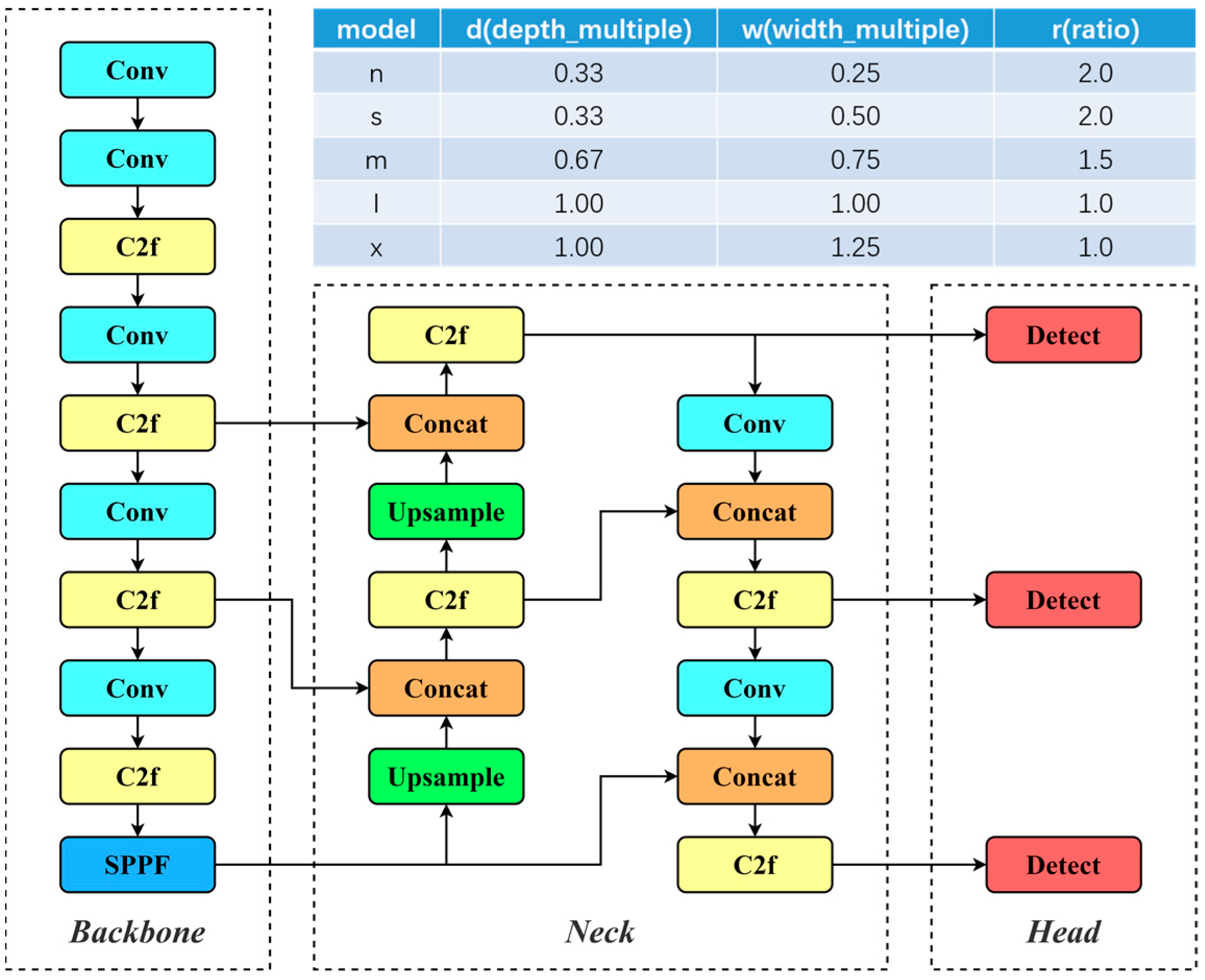
3. The Proposed Method

This paper has made improvements to YOLOv8, as depicted in Figure 4. The SimAM is added to the backbone network so that the model can focus more effectively on the important information in the input image and improve the performance and output effects of the model; the convolutional module of the neck is replaced by GhostConv, which reduces the redundant information, the number of model parameters, and computational complexity while retaining the model’s superior recognition performance; and the upsampling algorithm of the neck is replaced from the nearest interpolation to the bilinear interpolation, which provides a higher precision image.

3.1. SimAM

In deep learning, an attention mechanism is an approach that mimics the human visual and cognitive system. The attention mechanism assists the recommendation model in assigning varying weights to each part of the input, thereby extracting more crucial and significant information and enabling the recommendation model to make more precise assessments. It does not bring more overhead to the calculation and storage of the model [24], thereby enhancing the model’s performance and generalization ability.

Most existing attention modules typically generate one-dimensional or two-dimensional weights based on the feature X. As shown in Figure 5a,b, these generated weights are expanded into the channel attention mechanism and spatial attention mechanism to refine features in the channel or spatial dimensions. This approach limits their flexibility to learn different attention weights in both channel and spatial dimensions. Moreover, these mechanisms are often constructed based on a series of complex factors, such as the choice of pooling. This paper introduces the SimAM into the backbone network of YOLOv8. The SimAM is a straightforward, parameter-free plug-and-play module [25]. As shown in Figure 5c, it simultaneously considers channel and spatial dimensions, calculates three-dimensional weights through its own defined neuron energy function, and guides the model to focus more on important information with high energy and ignore noise information. This enhances the model’s performance and generalization ability without adding any parameters. The calculation steps of the SimAM are as follows:

SimAM directly infers three-dimensional weights from neurons and then refines these neurons in turn. SimAM defines the following energy function for each neuron:

$${\mathrm{e}}_t(w_t,b_t,y,x_i)={(y_t-\widehat{t})}^2+\frac{1}{M-1}{\displaystyle \sum _{i=1}^{M-1}{(y_0-{\widehat{x}}_i)}^2},$$

(1)

where $\widehat{t}=w_{t}t+b_t$ and ${\widehat{x}}_i=w_t{x}_i+b_t$ are linear transformations of $t$ and $x_i$, $t$ and $x_i$ are the target neuron and other neurons in a single channel of the input feature $X\in R^{C\times H\times W}$, $i$ is the index over the spatial dimension, $M=H\times W$ is the number of neurons on the channel, and $w_t$ and $b_t$ are the weight and bias transformations. All values in Equation (1) are scalars. Equation (1) reaches the minimum when $\widehat{t}$ is equal to $y_t$, all other values of ${\widehat{x}}_i$ are equal to $y_0$, and $y_t$ is not equal to $y_0$. Minimizing this equation allows us to find the linear separability between the target neuron $t$ and other neurons in the same channel. For simplicity, the final definition of the energy function is obtained by using binary labels (i.e., $y_t=1$ and $y_0=-1$) and adding regularization factors to Equation (1):

$${\mathrm{e}}_t(w_t,b_t,y,x_i)=\frac{1}{M-1}{\displaystyle \sum _{i=1}^{M-1}{(-1-(w_t{x}_i+b_t))}^2}+{(1-(w_{t}t+b_t))}^2+\lambda w_t^2.$$

(2)

The analytical solution obtained after simplifying the above formula is

$$w_t=-\frac{2(t-{\mu }_t)}{{(t-{\mu }_t)}^2+2{\sigma }_t^2+2\lambda },$$

(3)

$$b_t=-\frac{1}{2}\left(t+{\mu }_t\right)w_t,$$

(4)

where ${\mu }_t=\frac{1}{M-1}{\sum }_{i=1}^{M-1}{x}_i$ and ${\sigma }_t^2=\frac{1}{M-1}{\sum }_i^{M-1}{(x_i-{\mu }_t)}^2$ are the mean and variance computed for all neurons in the channel except for $t$. The minimum energy can be calculated employing the subsequent formula:

$$e_t^{\ast }=\frac{4({\widehat{\sigma }}^2+\lambda )}{{(t-\widehat{\mu })}^2+2{\widehat{\sigma }}^2+2\lambda },$$

(5)

where $\widehat{\mu }=\frac{1}{M}{\sum }_{i=1}^M{x}_i$ and ${\widehat{\sigma }}^2=\frac{1}{M}{\sum }_{i=1}^M{(x_i-\widehat{\mu })}^2$. Equation (5) indicates that the lower the energy $e_t^{\ast }$, the more distinct and linearly separable the neuron $t$ is from the peripheral neurons and the more important the neuron $t$ is for visual processing. The importance of each neuron can be expressed by $1/e_t^{\ast }$. Finally, the features are refined according to the definition of attentional mechanisms:

$$\tilde{X}=sigmoid\left(\frac{1}{E}\right)\odot X,$$

(6)

where $E$ is the grouping of all $e_t^{\ast }$ values across channel and spatial dimensions. Adding the sigmoid function prevents the value $E$ from being too large and does not affect the relative importance of each neuron.

3.2. GhostConv Convolution Module

Popular convolution modules often generate rich feature maps to guarantee a comprehensive comprehension of the input data. However, this inevitably leads to feature redundancy, resulting in unnecessary computational overhead. For the given input data $X\in R^{c\times h\times w}$, where $c$ is the number of input channels and $h$ and $w$ are the height and width of the input data, the operation of producing $\mathrm{n}$ feature maps by the conventional convolutional layer can be formulated as

$$Y=X\times f+b,$$

(7)

where $\ast$ is the convolution operation, $b$ is the bias term, $Y\in R^{h^{\prime }\times w^{\prime }\times n}$ is the output feature map with $\mathrm{n}$ channels, and $f\in R^{c\times k\times k\times n}$ are the convolution filters of the layer. Additionally, $h^{\prime }$ and $w^{\prime }$ are the height and width of the output data, and $k\times k$ is the kernel size of the convolution filters $f$. The required floating-point operations per second (FLOPs) during the convolution process are $n\cdot h^{\prime }\cdot w^{\prime }\cdot c\cdot k\cdot k$, and since the number of filters $\mathrm{n}$ and the number of channels $c$ are usually large, the FLOPs are also large.

To address this issue, in this paper, we replace the Conv module in the YOLOv8 neck network with GhostConv. GhostConv is a convolutional module from GhostNet, a lightweight network designed by Noah’s Ark Laboratory. Compared to regular convolutional neural networks, GhostConv decreases the number of parameters and computational complexity while maintaining the size of the output feature map. Additionally, it maintains superior recognition performance.

GhostConv first uses regular convolution to generate $m$ feature maps $Y^{\prime }\in R^{h^{\prime }\times w^{\prime }\times m}$:

$$Y^{\prime }=X\times f^{\prime },$$

(8)

where $f^{\prime }\in R^{c\times k\times k\times m}$ are the filters used, and $m\le n$ and the bias term are omitted for simplicity. To maintain the spatial size of the output feature map (i.e., $h^{\prime }$ and $w^{\prime }$), hyperparameters such as filter size, stride, padding, etc., are the same as those in the regular convolution (Equation (7)). To obtain the desired $\mathrm{n}$ feature maps, a series of inexpensive linear operations are applied to each intrinsic feature in $Y^{\prime }$. The $s$ ghosts are generated according to the following function:

$$y_{ij}={\Phi }_{i,j}(y_i^{\prime }),\forall i=1,\dots ,m,j=1,\dots ,s,$$

(9)

where $y_i^{\prime }$ is the $i$-th intrinsic feature map in $Y^{\prime }$, and ${\Phi }_{i,j}$ is the $j$-th (excluding the last one) linear operation for generating the $j$-th ghost feature map $y_{ij}$. In other words, $y_i^{\prime }$ can have one or more ghost feature maps ${\left\{y_{ij}\right\}}_{j=1}^s$. The final ${\Phi }_{i,s}$ is used to preserve the identity mapping of the intrinsic feature map. By using Equation (9), we can obtain $n=m\cdot s$ feature maps with $Y=\left[y_{11},y_{12},\dots ,y_{ms}\right]$ as the output of the ghost module, as illustrated in Figure 6.

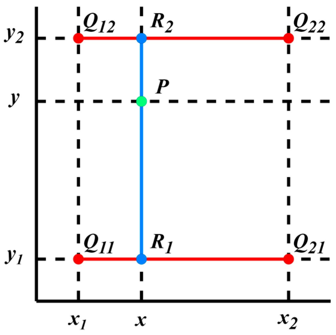
3.3. Bilinear Interpolation

In YOLOv8, nearest interpolation is used for upsampling and enlarging images. As shown in Figure 7, this method first reduces the target image to the size of the original image. Then, at that scale, for each pixel to be interpolated, it calculates its corresponding position in the original image, finds the closest pixel coordinates in the original image to the target position, and sets the pixel value at the target position to the value of the nearest neighbor pixel. Nearest interpolation is the simplest and requires the least processing time of all the interpolation algorithms [26]. However, nearest interpolation simply selects the nearest pixel value without considering the information of surrounding pixels, and it does not generate new pixel values. This results in the inability to achieve smooth transitions between pixels when performing upsampling operations, leading to jagged edges or blurred details in the image. This influence is particularly noticeable when dealing with detail-rich images and may lead to image distortion.

Therefore, this paper uses bilinear interpolation for the upsampling operation. Bilinear interpolation takes a weighted average of the four neighborhood pixels to calculate its final interpolated value [27], which better preserves details, resulting in smoother images and generating more realistic results. There are two alignment methods for bilinear interpolation, and the scaling ratios differ depending on the alignment method. As shown in Figure 8, bilinear interpolation scales the target image. In the corner alignment method, the center points of the pixels at the four corners of the target image align with the center points of the pixels at the four corners of the original image. In the edge alignment method, the sides of the target image align with the original image after scaling. The bilinear interpolation used in this paper employs the corner alignment method for computation. The calculation steps of bilinear interpolation are as follows.

As shown in Figure 9, assuming that we require the pixel value of point $P$ located at $(x,y)$ in the target image after scaling, and the pixel values of the four nearest original image points $Q_{11}$, $Q_{12}$, $Q_{21}$, and $Q_{22}$ to point $P$ are $(x_1,y_1)$, $(x_1,y_2)$, $(x_2,y_1)$, and $(x_2,y_2)$, respectively, the bilinear interpolation diagram could be formed as follows.

To begin with, linear interpolation is performed in the x-axis direction for $Q_{11}$, $Q_{21}$ and $Q_{12}$, $Q_{22}$, resulting in intermediate results $R_1(x,y_1)$ and $R_2(x,y_2)$:

$$f(x,y_1)=\frac{x_2-x}{x_2-x_1}f(Q_{11})+\frac{x-x_1}{x_2-x_1}f(Q_{21}),$$

(10)

$$f(x,y_2)=\frac{x_2-x}{x_2-x_1}f(Q_{12})+\frac{x-x_1}{x_2-x_1}f(Q_{22}).$$

(11)

After that, linear interpolation is performed on $R_1$, $R_2$ in the y-axis direction to obtain the pixel value of point $P$:

$$\begin{array}{l}f(x,y)=\frac{y_2-y}{y_2-y_1}f(x,y_1)+\frac{y-y_1}{y_2-y_1}f(x,y_2)\\ =\frac{y_2-y}{y_2-y_1}\left(\frac{x_2-x}{x_2-x_1}f(Q_{11})+\frac{x-x_1}{x_2-x_1}f(Q_{21})\right)+\frac{y-y_1}{y_2-y_1}\left(\frac{x_2-x}{x_2-x_1}f(Q_{12})+\frac{x-x_1}{x_2-x_1}f(Q_{22})\right)\\ =\frac{1}{(x_2-x_1)(y_2-y_1)}\left(f(Q_{11})(x_2-x)(y_2-y)+f(Q_{21})(x-x_1)(y_2-y)+f(Q_{12})(x_2-x)(y-y_1)+f(Q_{22})(x-x_1)(y-y_1)\right)\\ =\frac{1}{(x_2-x_1)(y_2-y_1)}\left[\begin{array}{cc}{x}_2-x& x-x_1\end{array}\right]\left[\begin{array}{cc}f(Q_{11})& f(Q_{12})\\ f(Q_{21})& f(Q_{22})\end{array}\right]\left[\begin{array}{c}{y}_2-y\\ y-y_1\end{array}\right]\end{array}.$$

(12)

4. Experimental Results and Analysis

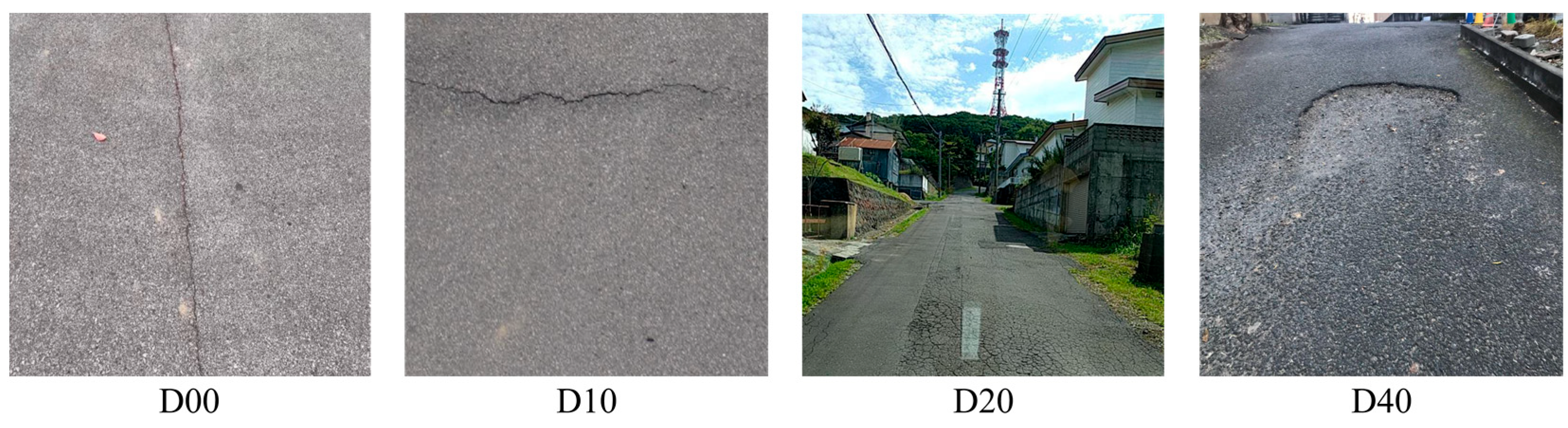
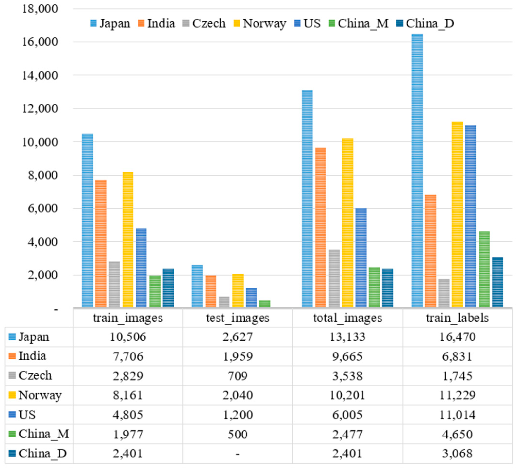
4.1. Dataset

This paper uses the RDD2022 dataset [28] from the open-source Crowdsensing-based Road Damage Detection Challenge (CRDDC’2022) [29] for model training. The RDD2022 dataset consists of 47,420 road images collected from six countries: Japan, India, the Czech Republic, Norway, the United States, and China. The dataset is prepared following the format of the PASCAL Visual Object Classes (VOC) datasets [30], with XML files providing annotations for over 55,000 instances of road damage. As illustrated in Figure 10, the dataset encompasses four damage types: longitudinal cracks (D00), transverse cracks (D10), alligator cracks (D20), and potholes (D40), with respective counts of 26,016, 11,830, 10,617, and 6544 instances. The distribution of these damage types reveals that longitudinal cracks are the most prevalent, while potholes are relatively less frequent.

The RDD2022 dataset is segmented into two sets: the training set and the test set. The distribution of images and labels across different countries in the dataset is illustrated in Figure 11. Images in the training set are accompanied by annotation files, while images in the test set do not include annotations. Therefore, the detection results need to be converted into files in a specific format and submitted to the CRDDC’2022 official website (https://crddc2022.sekilab.global/ (accessed on 1 March 2024)) for evaluation. Consequently, we divided the data from the RDD2022 training set into our experimental training set and validation set in a 7:3 ratio, using the RDD2022 test set as our experimental test set. We then tested the trained model on the test set and submitted the results to the official website to view the outcomes.

4.2. Experimental Environment

The experimental setup for our paper includes the following hardware and software configurations: The server operating system used is Ubuntu 18.04, equipped with an Intel(R) Xeon(R) E5-2667 v4 Central Processing Unit (CPU), and an NVIDIA RTX 4090 GPU with 24GB of VRAM. The training environment is configured with PyTorch 2.0.1, Python 3.8, and CUDA 11.7.

The experimental parameters in this paper are configured as follows: The input image resolution is set to 640 × 640, the initial learning rate is 0.01, the learning rate momentum is 0.937, and the Stochastic Gradient Descent (SGD) optimizer is used for training.

4.3. Evaluation Metrics

This paper refers to the evaluation metrics for road damage detection in CRDDC’2022, using the F1 score and mean average precision (mAP) to assess the performance of the trained model. The F1 score is the harmonic mean of precision and recall values; maximizing the F1 score ensures reasonably high precision and recall [31]. Precision is the ratio of true positives to all predicted positives, while recall is the ratio of true positives to all actual positives. Both precision and recall are based on the Intersection over Union (IoU) evaluation, described as the overlap area between the predicted bounding box and the true bounding box divided by their union area. It measures the degree of overlap between the predicted and true target boxes, as shown in Figure 12. Since precision and recall are contradictory, increasing one usually decreases the other. Therefore, the F1 score is employed as the final evaluation metric to balance both. mAP is the average of the average precision (AP) for different classes. This paper uses mAP50 and mAP50-95 metrics for evaluation. mAP50 represents the average precision at the IoU threshold of 0.5, and mAP50-95 is an extension of mAP50, indicating the average precision at different thresholds (from 0.5 to 0.95 with a step size of 0.05). It offers a comprehensive assessment of the model’s accuracy in predicting target boxes under different IoU thresholds. The detailed parameters are as follows:

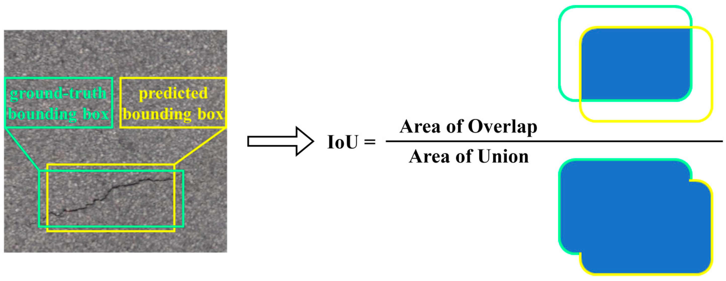
• True Positive (TP): An instance of road damage exists in the real situation and the labeling of the instance is correctly predicted, the overlap area between the predicted bounding box and the ground truth bounding box is more than 50%, and the IoU > 0.5.
• False Positive (FP): The model predicts an instance of road damage at the specific position in the image that does not exist in the ground reality of the image. FP includes cases where the predicted labels do not match the actual labels too.
• False Negative (FN): When there are instances of road damage in the real situation, but the model cannot predict the correct label or bounding box for the instance.
• Recall:

  $$Recall=\frac{TP}{TP+FN}.$$

  (13)
• Precision:

  $$Precision=\frac{TP}{TP+FP}.$$

  (14)
• F1 Score:

  $$F\mathsf{1}Score=2\frac{Precision\cdot Recall}{Precision+Recall}.$$

  (15)
• AP: The precision–recall (PR) curve $p(r)$ can be plotted based on precision and recall values, and the AP is the average value of the function $p(r)$ over the domain of definition $r\in [0,1]$.

  $$AP={\displaystyle {\int }_0^{1}p(r)dr}$$

  (16)
• mAP: Calculate and average the APs for each category.

  $$mAP=\frac{{\displaystyle {\sum }_{i=1}^{N}A{P}_i}}{N}$$

  (17)
• Params: The total quantity of learnable parameters in the neural network, including model weights and biases, is used to measure the spatial complexity and size of the model.
• Giga-FLOPs (GFLOPs): The quantity of billion floating-point operations performed by the model per second. GFLOPs is used to evaluate the computational complexity and efficiency of the model.

Figure 12. IoU calculation diagram.

Figure 12. IoU calculation diagram.

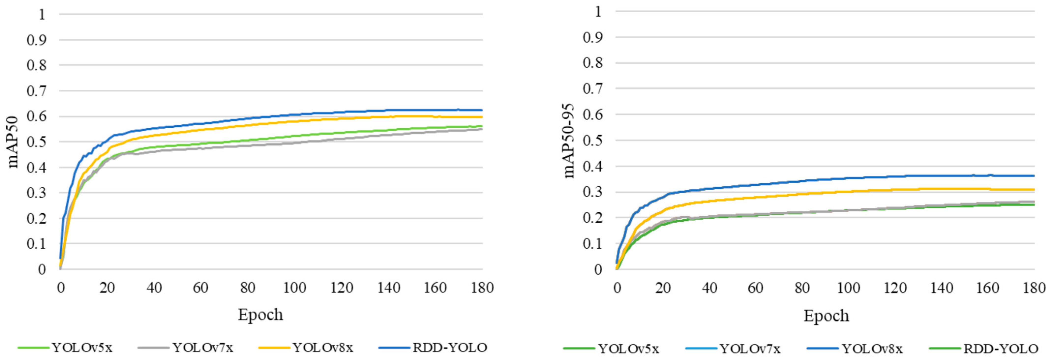
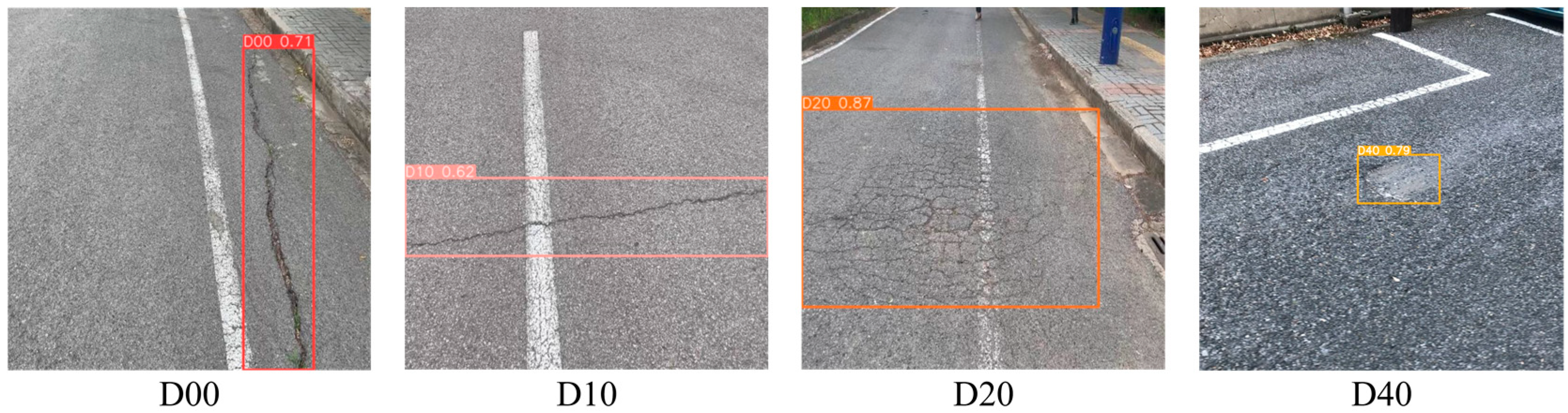
4.4. Experimental Implementation and Experimental Results

In pursuit of higher accuracy, this paper adopts YOLOv8x as the baseline and conducts comparative experiments using RDD-YOLO and other classic YOLO algorithms, with 180 rounds of training. Figure 13 displays the mAP50 and mAP50-95 curves on the validation set. We can observe that the performance of YOLOv5x and YOLOv7x are comparable, and the performance of YOLOv8x is relatively better. Compared with other YOLO algorithms, the proposed RDD-YOLO model has a faster convergence speed and higher values of mAP50 and mAP50-95.

The final mAP50 and mAP50-95 of RDD-YOLO and YOLOv8x on the validation set for different road damage categories can be seen in

Table 1. Comparison of road damage detection results for various types of roads in validation set.

Algorithms	Type	mAP50	mAP50-95
YOLOv8x	D00	59.3	33.3
	D10	59.7	30.1
	D20	67.7	37.7
	D40	52.9	23.9
	ALL	59.9	31.2
RDD-YOLO	D00	62.8 (+3.5)	38.8 (+5.5)
	D10	61.4 (+1.7)	35.2 (+5.1)
	D20	69.2 (+1.5)	42.3 (+4.6)
	D40	57.4 (+4.5)	30.1 (+6.2)
	ALL	62.5 (+2.6)	36.4 (+5.2)

. According to the data in the table, both RDD-YOLO and YOLOv8x exhibit the best detection performance for the D20 category, attributed to the distinct features of grid cracks. However, due to the irregular shape, small volume, and relatively fewer samples of potholes, the model’s detection performance for D40 is relatively lower. RDD-YOLO achieved final mAP50 and mAP50-95 scores of 62.8% and 36.7%, respectively, showing improvements of 2.6% and 5.2% over YOLOv8x. Specifically, there is a significant improvement in D40 detection, with an increase of 4.5% in mAP50 and 6.2% in mAP50-95. The model also exhibited notable improvements in detecting other types of road damage. RDD-YOLO enhances its ability to retain image details and focus on key information, leading to improved performance in road damage detection tasks.

For validating the performance of the algorithm presented in this paper, we compare RDD-YOLO with high-accuracy models such as YOLOv5x, YOLOv7x, and YOLOv8x proposed in recent years. Additionally, we introduce p-YOLOv5x for comparison, a model that uses pre-trained weights from the winning solution in the Global Road Damage Detection Challenge (GRDDC’2020) [32] proposed by Hegde V et al. [33]. As illustrated in

Table 2. Comparison results of different algorithms.

Model	F1 (India)	F1 (Japan)	F1 (United States)	F1 (6 Countries)	Params/M	GFLOPs
YOLOv5x	44.9	63.5	68.0	63.6	88.5	220.5
p-YOLOv5x	46.8	64.5	63.2	60.0	88.5	220.5
YOLOv7x	42.1	62.0	68.1	62.6	70.8	188.9
YOLOv8x	43.6	66.3	71.5	66.8	68.2	258.1
RDD-YOLO	53.0	70.2	73.6	69.6	65.9	255.3

, the comparison reveals that higher versions of YOLO models have a smaller parameter count compared to lower versions, and the YOLOv8x model outperforms lower versions in terms of performance. The p-YOLOv5x, utilizing pre-trained weights from the winning solution in GRDDC’2020, performs well on the Indian and Japanese datasets due to the use of RDD2020 [34], which includes images only from Japan, India, and the Czech Republic. However, its overall F1 score is still lower compared to YOLOv5x. Notably, the proposed RDD-YOLO performs excellently on both overall and individual country datasets, exhibiting superior performance and having a smaller parameter count. Although RDD-YOLO has a smaller number of GFLOPS compared to YOLOv8x, it is still larger than other models, possibly requiring more computational resources and time. In summary, RDD-YOLO excels in both performance and model parameters, surpassing other models. This research result provides strong support for future studies and practical applications.

To further validate the effectiveness of the introduced improvements on the RDD-YOLO model, a series of ablation experiments were conducted, as shown in

Table 3. Model improvement ablation experiment.

Model	SimAM	GhostConv	Bilinear	F1	Params/M	GFLOPs
YOLOv8x				66.8	68.2	258.1
YOLOv8-S	√			68.3	68.2	258.1
YOLOv8-G		√		67.1	65.9	255.2
YOLOv8-B			√	67.4	68.2	258.1
RDD-YOLO	√	√	√	69.6	65.9	255.3

. By comparing the experimental results, it can be found that the introduced improvements have a positive impact on model performance while almost not affecting the model size and inference speed. First of all, based on the experimental results, it can be discovered that the SimAM and the replaced bilinear interpolation in this paper improved the F1 score of the original model by 1.5 and 0.6 percentage points, respectively. This indicates that by introducing these improvements into the model structure, we can significantly enhance the model’s detection capability for road damage, and these improvements do not increase the model’s complexity and computational overhead. Secondly, the GhostConv structure introduced in this paper not only improved the F1 score by 0.3% but also reduced a certain amount of model parameters and computations. In the end, considering all improvements, the proposed method in this paper achieved a 2.8% increase in F1 score in contrast with the baseline model YOLOv8x. While ensuring detection accuracy, there was also a certain degree of reduction in model parameters and computations.

Figure 14 shows the detection performance of our model on the test set for road damage. Different subplots correspond to four common types of road damage mentioned above. Through the observation of these subplots, we can deduce some important features of the detection results. Firstly, for alligator cracks and road potholes, due to their relatively distinct features, we can observe high confidence scores for the predicted boxes. This indicates that our model performs well in detecting these more obvious damage types and accurately marks their positions. However, longitudinal cracks and transverse cracks are usually characterized as very small and narrow. Due to the more detailed morphology of these cracks, the model tends to exhibit relatively lower confidence during detection. Nevertheless, the model in this paper still shows satisfactory performance, being able to locate and fit these cracks with more elongated morphology more accurately. Overall, our model performs well with different shapes of cracks and shows good generalization. Our model is not only able to adapt to the more obvious and common types of damage but is also able to deal with the more detailed cracks, providing a reliable solution for the comprehensive detection of road damage. This is of positive significance for ensuring road safety.

5. Conclusions

To enhance the precision of road damage detection and minimize the labor and material expenses associated with road damage assessment and maintenance, this paper proposes a road damage detection algorithm based on improved YOLOv8, named RDD-YOLO. This algorithm introduces several key optimization measures to improve model performance. To start with, the SimAM is introduced into the backbone network to enhance the focus on key information in the input image. This allows the model to selectively concentrate on critical areas in the input image, enabling more effective capture of relevant features related to road damage and significantly improving detection accuracy. Furthermore, an optimization is applied to the neck structure by replacing the traditional convolution module with GhostConv. This change achieves a more lightweight and efficient performance in the damage detection task while maintaining excellent performance in recognizing damage. Lastly, the upsampling algorithm of the neck is improved by replacing the nearest interpolation with bilinear interpolation, which better restores the subtle features of the image and improves the accuracy of the detection results through a finer interpolation method. Experimental results demonstrate that RDD-YOLO achieves an F1 score of 69.6% on the RDD2022 dataset, surpassing other algorithms not only in detection performance but also with more concise parameters. Although RDD-YOLO performs well, there is still room for improvement: the variety of road damage types, in reality, is extensive, while RDD2022 covers only four common types of road damage. Therefore, our model can only identify these four types of road damage. Additionally, in pursuit of higher F1 scores, we chose the large-scale YOLOv8x as the baseline model, which, despite improvements to reduce parameter count to some extent, remains quite large and may be challenging to deploy on resource-constrained, high real-time demand mobile endpoint devices. Moving forward, we will seek more comprehensive datasets to identify a greater variety of road damage types, further optimize network models, reduce model size and complexity, increase detection speed, and strive to further improve detection accuracy, enabling the model to be better applied to practical tasks such as road surface crack detection.

References

1. Available online: https://baike.baidu.hk/item/%E5%85%AC%E8%B7%AF/7265058 (accessed on 3 April 2024).
2. Yang, L.; Zhang, R.-Y.; Li, L.; Xie, X. SimAM: A Simple, Parameter-Free Attention Module for Convolutional Neural Networks. In Proceedings of the 38th International Conference on Machine Learning; PMLR, Virtual Event, 18–24 July 2021; pp. 11863–11874. [Google Scholar]
3. Han, K.; Wang, Y.; Tian, Q.; Guo, J.; Xu, C.; Xu, C. Ghostnet: More Features from Cheap Operations. In Proceedings of the IEEE/CVF Conference on Computer Vision and Pattern Recognition, Seattle, WA, USA, 14–19 June 2020; pp. 1580–1589. [Google Scholar]
4. Lim, R.S.; La, H.M.; Shan, Z.; Sheng, W. Developing a Crack Inspection Robot for Bridge Maintenance. In Proceedings of the 2011 IEEE International Conference on Robotics and Automation, Shanghai, China, 9–13 May 2011; IEEE: Piscataway, NJ, USA, 2011; pp. 6288–6293. [Google Scholar]
5. Kapela, R.; Śniatała, P.; Turkot, A.; Rybarczyk, A.; Pożarycki, A.; Rydzewski, P.; Wyczałek, M.; Błoch, A. Asphalt Surfaced Pavement Cracks Detection Based on Histograms of Oriented Gradients. In Proceedings of the 2015 22nd International Conference Mixed Design of Integrated Circuits & Systems (MIXDES), Torun, Poland, 25–27 June 2015; pp. 579–584. [Google Scholar]
6. Wang, G.-L.; Hu, J.; Qian, J.-G.; Wang, Y.-Q. Simulation in Time Domain for Nonstationary Road Disturbances and Its Wavelet Analysis. Zhendong Yu Chongji (J. Vib. Shock) 2010, 29, 28–32. [Google Scholar]
7. Fan, Z.; Wu, Y.; Lu, J.; Li, W. Automatic Pavement Crack Detection Based on Structured Prediction with the Convolutional Neural Network. arXiv 2018, arXiv:1802.02208. [Google Scholar]
8. Cao, M.-T.; Tran, Q.-V.; Nguyen, N.-M.; Chang, K.-T. Survey on Performance of Deep Learning Models for Detecting Road Damages Using Multiple Dashcam Image Resources. Adv. Eng. Inform. 2020, 46, 101182. [Google Scholar] [CrossRef]
9. Kang, D.; Benipal, S.S.; Gopal, D.L.; Cha, Y.-J. Hybrid Pixel-Level Concrete Crack Segmentation and Quantification across Complex Backgrounds Using Deep Learning. Autom. Constr. 2020, 118, 103291. [Google Scholar] [CrossRef]
10. Mandal, V.; Mussah, A.R.; Adu-Gyamfi, Y. Deep Learning Frameworks for Pavement Distress Classification: A Comparative Analysis. In Proceedings of the 2020 IEEE International Conference on Big Data (Big Data), Atlanta, GA, USA, 10–13 December 2020; pp. 5577–5583. [Google Scholar]
11. Chen, Q.; Gan, X.; Huang, W.; Feng, J.; Shim, H. Road Damage Detection and Classification Using Mask R-CNN with DenseNet Backbone. Comput. Mater. Contin. 2020, 65, 2201–2215. [Google Scholar] [CrossRef]
12. Yuan, Y.; Yuan, Y.; Baker, T.; Kolbe, L.M.; Hogrefe, D. FedRD: Privacy-Preserving Adaptive Federated Learning Framework for Intelligent Hazardous Road Damage Detection and Warning. Future Gener. Comput. Syst. 2021, 125, 385–398. [Google Scholar] [CrossRef]
13. Zhang, Y.; Zuo, Z.; Xu, X.; Wu, J.; Zhu, J.; Zhang, H.; Wang, J.; Tian, Y. Road Damage Detection Using UAV Images Based on Multi-Level Attention Mechanism. Autom. Constr. 2022, 144, 104613. [Google Scholar] [CrossRef]
14. Wang, J.; Gao, X.; Liu, Z.; Wan, Y. GSC-YOLOv5: An Algorithm Based on Improved Attention Mechanism for Road Creak Detection. In Proceedings of the 2023 IEEE 12th Data Driven Control and Learning Systems Conference (DDCLS), Xiangtan, China, 12–14 May 2023; IEEE: Washington, DC, USA, 2023; pp. 1664–1671. [Google Scholar]
15. Ni, Y.; Mao, J.; Fu, Y.; Wang, H.; Zong, H.; Luo, K. Damage Detection and Localization of Bridge Deck Pavement Based on Deep Learning. Sensors 2023, 23, 5138. [Google Scholar] [CrossRef] [PubMed]
16. Redmon, J.; Divvala, S.; Girshick, R.; Farhadi, A. You Only Look Once: Unified, Real-Time Object Detection. In Proceedings of the IEEE Conference on Computer Vision and Pattern Recognition, Las Vegas, NV, USA, 21–26 July 2016; pp. 779–788. [Google Scholar]
17. Xiao, B.; Nguyen, M.; Yan, W.Q. Fruit Ripeness Identification Using YOLOv8 Model. Multimed. Tools Appl. 2024, 83, 28039–28056. [Google Scholar] [CrossRef]
18. Redmon, J.; Farhadi, A. YOLO9000: Better, Faster, Stronger. In Proceedings of the IEEE Conference on Computer Vision and Pattern Recognition, Honolulu, HI, USA, 21–26 July 2017; pp. 7263–7271. [Google Scholar]
19. Redmon, J.; Farhadi, A. YOLOv3: An Incremental Improvement. arXiv 2018, arXiv:1804.02767. [Google Scholar]
20. Bochkovskiy, A.; Wang, C.-Y.; Liao, H.-Y.M. YOLOv4: Optimal Speed and Accuracy of Object Detection. arXiv 2020, arXiv:2004.10934. [Google Scholar]
21. Hussain, M. YOLO-v1 to YOLO-v8, the Rise of YOLO and Its Complementary Nature toward Digital Manufacturing and Industrial Defect Detection. Machines 2023, 11, 677. [Google Scholar] [CrossRef]
22. Li, C.; Li, L.; Jiang, H.; Weng, K.; Geng, Y.; Li, L.; Ke, Z.; Li, Q.; Cheng, M.; Nie, W.; et al. YOLOv6: A Single-Stage Object Detection Framework for Industrial Applications. arXiv 2022, arXiv:2209.02976. [Google Scholar]
23. Wang, C.-Y.; Bochkovskiy, A.; Liao, H.-Y.M. YOLOv7: Trainable Bag-of-Freebies Sets New State-of-the-Art for Real-Time Object Detectors. In Proceedings of the IEEE/CVF Conference on Computer Vision and Pattern Recognition, Vancouver, BC, Canada, 18–22 June 2023; pp. 7464–7475. [Google Scholar]
24. Gao, G.-S. Survey on Attention Mechanisms in Deep Learning Recommendation Models. Comput. Eng. Appl. 2022, 58, 9–18. [Google Scholar]
25. Zhang, Y.; Shen, S.; Xu, S. Strip Steel Surface Defect Detection Based on Lightweight YOLOv5. Front. Neurorobot. 2023, 17, 1263739. [Google Scholar] [CrossRef] [PubMed]
26. Parsania, P.-S.; Virparia, P.-V. A Comparative Analysis of Image Interpolation Algorithms. Int. J. Adv. Res. Comput. Commun. Eng. 2016, 5, 29–34. [Google Scholar] [CrossRef]
27. Patel, V.; Mistree, K. A Review on Different Image Interpolation Techniques for Image Enhancement. Int. J. Emerg. Technol. Adv. Eng. 2013, 3, 129–133. [Google Scholar]
28. Arya, D.; Maeda, H.; Ghosh, S.K.; Toshniwal, D.; Sekimoto, Y. RDD2022: A Multi-National Image Dataset for Automatic Road Damage Detection. arXiv 2022, arXiv:2209.08538. [Google Scholar]
29. Arya, D.; Maeda, H.; Ghosh, S.K.; Toshniwal, D.; Omata, H.; Kashiyama, T.; Sekimoto, Y. Crowdsensing-Based Road Damage Detection Challenge (CRDDC’2022). In Proceedings of the 2022 IEEE International Conference on Big Data (Big Data), Osaka, Japan, 17–20 December 2022; IEEE: Washington, DC, USA, 2022; pp. 6378–6386. [Google Scholar]
30. Everingham, M.; Eslami, S.M.A.; Van Gool, L.; Williams, C.K.I.; Winn, J.; Zisserman, A. The Pascal Visual Object Classes Challenge: A Retrospective. Int. J. Comput. Vis. 2015, 111, 98–136. [Google Scholar] [CrossRef]
31. Arya, D.; Maeda, H.; Ghosh, S.K.; Toshniwal, D.; Mraz, A.; Kashiyama, T.; Sekimoto, Y. Transfer Learning-Based Road Damage Detection for Multiple Countries. arXiv 2020, arXiv:2008.13101. [Google Scholar]
32. Arya, D.; Maeda, H.; Kumar Ghosh, S.; Toshniwal, D.; Omata, H.; Kashiyama, T.; Sekimoto, Y. Global Road Damage Detection: State-of-the-Art Solutions. In Proceedings of the 2020 IEEE International Conference on Big Data (Big Data), Atlanta, GA, USA, 10–13 December 2020; pp. 5533–5539. [Google Scholar]
33. Hegde, V.; Trivedi, D.; Alfarrarjeh, A.; Deepak, A.; Ho Kim, S.; Shahabi, C. Yet Another Deep Learning Approach for Road Damage Detection Using Ensemble Learning. In Proceedings of the 2020 IEEE International Conference on Big Data (Big Data), Atlanta, GA, USA, 10–13 December 2020; pp. 5553–5558. [Google Scholar]
34. Arya, D.; Maeda, H.; Ghosh, S.K.; Toshniwal, D.; Sekimoto, Y. RDD2020: An Annotated Image Dataset for Automatic Road Damage Detection Using Deep Learning. Data Briefs 2021, 36, 107133. [Google Scholar] [CrossRef]
Figure 1. Object detection algorithm classification.
Applsci 14 03360 g001
Figure 2. YOLO algorithm evolution timeline [16,18,19,20,22,23].
Applsci 14 03360 g002
Figure 3. YOLOv8 network architecture.
Applsci 14 03360 g003
Figure 4. Improved YOLOv8 network architecture.
Applsci 14 03360 g004
Figure 5. Comparisons of different attention in different dimensions [2]. The identical color signifies the use of a sole scalar applied to every channel, spatial position, or individual point across those features.
Applsci 14 03360 g005
Figure 6. Comparisons of Conv and GhostConv [3]. (a) The convolutional layer. (b) The Ghost module.
Applsci 14 03360 g006
Figure 7. Nearest interpolation diagram.
Applsci 14 03360 g007
Figure 8. Comparison diagram of corner alignment and edge alignment.
Applsci 14 03360 g008
Figure 9. Bilinear interpolation diagram.
Applsci 14 03360 g009
Figure 10. Example images for road damage categories.
Applsci 14 03360 g010
Figure 11. RDD2022 data statistics: distribution of images and labels based on countries.
Applsci 14 03360 g011
Figure 13. mAP50 and mAP50-95 curves of different YOLO algorithms in validation set.
Applsci 14 03360 g013
Figure 14. Sample images of road damage detection for each category.
Applsci 14 03360 g014