Prediction of Total Petroleum Hydrocarbons and Heavy Metals in Acid Tars Using Machine Learning

Featured Application

Python application that uses data science and machine learning to estimate the main properties of acid tars. Its main advantage is that determinations for acid tar properties are no longer necessary, thus saving time and money. However, good machine learning estimations are highly dependent on the number and quality of the training data, meaning that the larger and more consistent the training database, the better the estimations.

Abstract

Hazardous petroleum wastes are an inevitable source of environmental pollution. Leachates from these wastes could contaminate soil and potable water sources and affect human health. The management of acid tars, as a byproduct of refining and petrochemical processes, represented one of the major hazardous waste problems in Romania. Acid tars are hazardous and toxic waste and have the potential to cause pollution and environmental damage. The need for the identification, study, characterization, and subsequently either the treatment, valorization, or elimination of acid tars is determined by the fact that they also have high concentrations of hydrocarbons and heavy metals, toxic for the storage site and its neighboring residential area. When soil contamination with acid tars occurs, sustainable remediation techniques are needed to restore soil quality to a healthy production state. Therefore, it is necessary to ensure a rapid but robust characterization of the degree of contamination with hydrocarbons and heavy metals in acid tars so that appropriate techniques can then be used for treatment/remediation. The first stage in treating these acid tars is to determine its properties. This article presents a software program that uses machine learning to estimate selected properties of acid tars (pH, Total Petroleum Hydrocarbons—TPH, and heavy metals). The program uses the Automatic Machine Learning technique to determine the Machine Learning algorithm that has the lowest estimation error for the given dataset, with respect to the Mean Average Error and Root Mean Squared Error. The chosen algorithm is used further for properties estimation, using the R² correlation coefficient as a performance criterion. The dataset used for training has 82 experimental points with continuous, unique values containing the coordinates and depth of acid tar samples and their properties. Based on an exhaustive search performed by the authors, a similar study that considers machine learning applications was not found in the literature. Further research is required because the method presented therein can be improved because it is dataset dependent, as is the case with every ML problem.

1. Introduction

The diversity of the operations and increasing growth of the petroleum industry has resulted in huge amounts of various waste materials that need proper disposal and/or valorization [1,2]. Among the existing types of petroleum waste, this paper studied the acid tars from a refinery storage lagoon in Romania. Acid tars are residual materials that result from refining and petrochemical technologies applied at the beginning of the oil industry development and which, by now, are abandoned [3,4,5].

Once formed, acid tars were stored in large-scale pits the size of a football field, called lagoons, which thus became permanent and potential pollution sources for the air, soil, subsoil, and water [6,7,8].

In addition to countries such as the USA, Russia, United Kingdom, Netherlands, Belgium, Germany, Latvia, Slovenia, Slovakia, China, Zimbabwe, and Ukraine, which store acid tar in the open air in spent pits, storage ponds, lagoons, or near landfills, there is also Romania [7,8,9]. On the problem of ATLs, scientific reports can be found in the literature, for example, in the USA, Germany, Belgium, Russia, UK, Slovenia, France, Latvia and Ukraine while the extent of the problem has not been limited to these countries [4,5,7,8].

The reason for conducting the research developed and described in this article is the historical existence of acid tar lagoons in five refineries in Prahova County, four being in the immediate vicinity of Ploiesti city, refineries put into operation at the beginning of the 20th century [9,10,11]. At present, although the quantity of acid tars generated has been greatly reduced due to the development of efficient catalytic processes in the refining industry, an effective treatment method is needed for existing acid tars lagoons [6].

The composition of the acid tars stored in the lagoons varies with the period of production, the product treated with sulfuric acid, and the age of the tars [12,13,14,15]. Acid tars have a variable composition between sites and even within one lagoon [15]. The need to study, characterize, and stabilize/dispose of the acid tars from these huge storage lagoons is determined by the fact that they have an extreme acidity (pH 1–2), high concentrations of hydrocarbons and heavy metals, with significant mobility and easily leachable, dangerous for the storage site and its neighboring residential area [7,8,15]. The low pH is an important chemical factor that influences the increase in the mobility of metals and their interaction with natural minerals [16].

Milne [3], Frolov et al. [12], Nieuwenhuis [17], and especially Kolmakov et al. [5,13] and other [18,19] reviewed various methods for the processing of acid tars into useful products but concluded that none of the approaches are satisfactory and thus, it is necessary to apply an effective remediation method of acid tars lagoons [20,21,22,23,24].

Evaluation and choosing a technology for the remediation of acid tar lagoons is a complex activity that requires the consideration of numerous factors: the type and properties of the emerging contaminants, their quantity, the dynamics of the pollutants, the hydrogeological characteristics of the soil, the climatic factors [8,9,15]. Finally, the economic aspects, namely the costs of remediation, also matter.

This work is associated with complex research that refers to a composition and process for the physical and chemical stabilization, in situ, of acid tars and of soil contaminated with acid tar from one selected lagoon through neutralizing, stabilization, and encapsulation procedure [25,26]. Acid tar samples from the studied lagoon were sampled, and the following steps were taken:

• Acid tar and leachate analysis from the stabilized tars is done by determining the following indicators: pH, TPH, and metals content, as well as As.
• Identification, testing, and determination of the optimal recipes for stabilizing the acid tar in the lagoon.
• Characterization of stabilized tar leachate and classifying it according to the Council Decision of December 2002 and Romanian Ministry Order 95 12 February 2005 [27].
• The identification of the conditions for the capitalization of the research and the obtained results for the treatment of the acid tars in the studied lagoon.

The characterization of untreated and treated acid tars in each site is conventionally accomplished through expensive sampling and testing of numerous borehole samples using highly sensitive and specific analytical procedures involving extraction and subsequent gravimetric or chromatographic techniques [4,13,28]. These procedures are laborious, expensive, time-consuming, and inadequate when high spatial and temporal resolutions of petroleum hydrocarbon content are required [15].

To overcome these limitations, a machine learning model was used in this work to predict pH, petroleum hydrocarbon concentrations, heavy metals, and As in the source area. The presented method estimates some selected properties of acid tar (pH, TPH, five heavy metals and a metalloid—As) based on the geographical location and depth of where the sample was taken. To achieve this purpose, a training database was created that contains data from other acid tar samples whose geographic coordinates and depth are already known. The Automatic Machine Learning technique determines the algorithm that offers the best estimation (smallest error) for every acid tar property that was estimated. Eight response variables from the field survey and database were considered as output variables for machine learning to train and test the models.

Artificial intelligence (AI) represents the simulation of human intelligence by computing machines, which are programmed to think and act as a human would [29]. AI is presented in different forms in our everyday lives in fields like games, stock market predictions, aeronautics, or electronic commerce.

The application of AI is an important issue in chemical, process, and petroleum engineering. Thus, they have been widely used in various applications in the chemical engineering field, including modeling, process control, classification, fault detection, and diagnosis [30]. The application of AI in important issues in oilfield development, including oilfield production dynamic prediction, developing plan optimization, residual oil identification, fracture identification, and enhanced oil recovery [31]. Also, with AI, refineries can leverage large datasets to help provide analytics that produce actionable insights [32,33].

In a similar manner, artificial intelligence and machine learning are essential to controlling or managing land contamination through prediction, clustering, data-centric analysis, and soil quality evaluation [34,35].

The prediction of soil petroleum hydrocarbon concentration is achieved by machine learning and the resistivity tomography method [36]. Since the field measurement of soil heavy metal content involves significant costs, methods have been developed to estimate soil heavy metals based on remote sensing images and machine learning [37,38,39]. Also, some measurements were studied and published using machine learning predictions of soil pH [40].

Unfortunately, there is limited research on predicting soil pollution, let alone the hydrocarbons and heavy metal content of acid tar lagoons; most research estimates air and water pollution. The concentration of hydrocarbons, heavy metals, and soil acidity does not change significantly without appropriate remedial measures, and this is based on the knowledge of the level of contamination of the soil with these contaminants. There have been numerous studies worldwide on the qualitative analysis, prevention and control, and remediation of soil pollution; however, there have been few studies on the quantitative analysis of soil pollution. It has become extremely important to evaluate and accurately predict the content of hydrocarbons and heavy metals in soil via acid tars lagoons.

The selected parameters in the present application of ML (pH, TPH and the content of heavy metals and As) have not been fully studied and correlated in any other study regarding, first of all, the initial composition of the acid tars in the lagoon and their values after the application’s stabilization-encapsulation procedure. Artificial intelligence with machine learning has never been applied before to measure the pH, TPH, and heavy metal content of acid tar in a lagoon. The lack of data was noted while it was being obtained. I specified that, with the exception of a few works in the literature, the uses of ML algorithms are published separately for soil pH, TPH, and heavy metals [34,35,36,37,38]. We specified that with the exception of a few works in the literature, the uses of the ML algorithm are published separately for soil pH, TPH, and heavy metals. Among the chemical substances identified in the potentially concerning acid tars under study in this paper, the concentrations of TPH and metals were determined experimentally and then estimated.

2. Materials and Methods

Sampling, preparation, and coding of the acid tar samples from the lagoon. The sampling procedure was done according to BS EN 14899:2005. Characterization of waste. Sampling of waste materials. Framework for the preparation and application of a sampling plan. This method is applicable for samples of untreated acid tar, neutralized tar, or stabilized tar in force (Order no. 95/2005).

Experimental layout. A lagoon area of 10.55 ha was used for this study. Sampling was carried out in acid tar sampling points from 5 cm, respectively, 30 cm depth, and following the STEREO 70 coordinates of the sampling points.

The characterization of the acid tar and the finite treated products was made by the determination of the following key indicators: pH, THP content, metals, chlorides, dissolved organic carbon (DOC), sulfites, total of dissolved solids (TDS), and total of organic carbon (TOC) [26]. According to Order 95 from 2005, to be deposited and accepted in deposits, the waste must have certain chemical properties [27]. This is why a specific analysis was conducted for the studied and treated acid tars. Also, the validation of the treatment process necessitated the performing of the leachate test.

Treatability testing program. The treatability studies specific to the studied lagoon and studies performed at a laboratory scale offered the necessary data for feasibility treatment recipe determination.

The working program had the following steps [26]:

• Sample collection;
• Initial samples characterization;
• Sample homogenization;
• Performing the chemical tests;
• Performing the treatability tests;
• Performing the test by mixing the reactants with the contaminated material and the formulation preparation for the next tests;
• Blending the design optimization;
• Selection of the mixture design verifying phase;
• Design and final test preparation;
• Data analysis, evaluation, and validation of recipes proposed and applied to the studied acid tars.

Laboratory analysis

Determining the TPH content. The determination of the TPH content was made using the gas-chromatographic method (GC-FID), according to the SR EN ISO 16703:2011 testing method.

Heavy metals and As concentrations. Metal concentrations were established according to the SR EN ISO 15586:2004 Analysis Method: Determination of Trace Elements by Graphite Furnace Atomic Absorption Spectrometry using a Graphite Furnace Atomic Absorption Spectrometer.

Our proprietary acid tar stabilization technology consists of the following [25,26]:

• Mixing the acid tar with powdered hydrated lime by bringing the pH to alkaline values (pH = 9–10) and passing the heavy metals into insoluble combinations, following the neutralization reaction with additives to stabilize the pH.
• The solidification and stabilization of acid tar by mixing with hydraulic binders and emulsifiers, which produces the encapsulation of contaminants in granular and uniform particles, blocking the possibility of their spreading in the environment.

The final validation of the recipes proposed and applied to the acid tar in the studied lagoon is being done by comparing the leachate/eluate indicators with the maximum allowed values for the leachate obtained from the acid tar, according to Order 95/2005 [27].

3. Machine Learning Algorithm Description

During the investigation, monitoring, and remediation of a site polluted with acid tars, the concentration of pollutants is an important factor in identifying the pollution level and spatial distribution [28].

Determining the treatment/elimination technologies of acid tars from the refineries and evaluating their feasibility was done by laboratory testing. Among the most important indicators of an acid tar sample and after applying the required treatment test, this paper focuses on the following: pH, TPH content, and heavy metals contents (Pb, Cd, Cu, Cr, Ni) and As.

A software program was developed to estimate the properties of new acid tar samples without measuring them. It was written in Python 3.11.6, using PyCharm Community Edition as IDE [41].

The developed software uses machine learning techniques to estimate the following eight properties of acid tars:

• Initial pH of the acid tar sample;
• Total Petroleum Hydrocarbons (TPH) of the acid tar;
• Initial lead concentration of the acid tar (mg/kg);
• Initial cadmium concentration of the acid tar (mg/kg);
• Initial copper concentration of the acid tar (mg/kg);
• Initial chrome concentration of the acid tar (mg/kg);
• Initial nickel concentration of the acid tar (mg/kg);
• Initial arsenic concentration of the acid tar (mg/kg).

These eight properties are the dependent or response variables.

The following properties are the predictor variables:

• The X- and Y-coordinates of the places where the soil samples were extracted. The stereographic 70 projection was used to represent those coordinates.
• The tar samples extraction depth (cm). A total of 82 samples were extracted either from 5 cm depth or 30 cm depth (41 samples each for the two depths of 5 and 30 cm).

The algorithm used for the developed program was taken from [42]. It is the preferred method of the authors because it is simple to understand and implement. The chosen method has the following steps:

• Obtaining the data.
• Data visualization.
• Preparing the data for the machine learning model.
• Selecting and training a machine learning model.
• Hyperparameter tuning.
• Evaluating the model on the test set.

Obtaining the data. This step involves obtaining the available data, which will be used for training the chosen algorithm. The data set contains 82 samples with the predictor and response variables mentioned above. Each row represents an acid tar sample, and each column represents one of the variables involved in this machine-learning project.

The main statistical characteristics of every acid tar sample property are presented in

Table 1. Main statistical characteristics of every acid tar sample property.

Property	Minimum Value	Maximum Value	Mean Value	Standard Deviation
X-coordinate	385,380.6	385,533.507	385,451.47	45.96
Y-coordinate	581,167.73	581,268.73	581,213.77	30.42
Sample depth	5	30	17.5	12.58
Initial pH	0.2	5.28	1.12	1.12
TPH	48,333	477,062	169,685.37	80,568.12
Initial Pb concentration	42	2235	343.07	372.91
Initial Cd concentration	1	126	20.34	19.82
Initial Cu concentration	5	789	46.59	101.9
Initial Cr concentration	3	452	27.35	60.51
Initial As concentration	1.4	589	96.13	137.37
Initial Ni concentration	2	859	28.5	109.67

.

After the data were obtained, it was divided into training and testing data. A total of 70% was used as training data, and 30% was used as testing data.

Data visualization is the next step. Its purpose is to offer visual insight into the obtained data, which may assist in solving the machine learning problem.

The geographic coordinates of the obtained samples are presented in Figure 1.

Figure 1 shows that the samples were taken from a well-defined, enclosed area. This means that there is a very high chance for the data to be consistent, and it will be helpful for future versions of the program to obtain training data from inside the area.

The following steps can be performed either manually or automatically. In the first option, the people conducting the machine learning make every choice along the way and write the appropriate lines of code. In the second case, the computer is responsible for making every decision and choice based on mathematical and statistical criteria. This technique is called “AutoML” (which comes from “Automatic Machine Learning”).

For the development of the machine learning software, Automatic Machine Learning was chosen by the authors for the following reasons:

• Automation and speed;
• Efficiency;
• Reduced human bias;
• Coding volume.

To implement AutoML, the PyCaret library was used. PyCaret is an open-source machine-learning library in Python that automates ML workflows [43]. This library automates the entire workflow, testing a very large number of algorithms and possibilities in a short amount of time. Because everything is automated, the results are objectively the best as they are chosen through mathematical and statistical values.

The parameters used in the PyCaret library are the default parameters unless specified otherwise.

Also, it is worth noting that PyCaret does not accept multivariate estimation. This means the next steps were executed for every response variable considered.

Preparing the data for the machine learning model is a very important step, which is essential for ensuring the accuracy, performance, and effectiveness of machine learning algorithms. It helps improve the quality and usability of the resulting insights and predictions.

For the training data obtained, the only data preparation needed was normalizing the predictor data for both the training and testing sets. The following normalization methods were chosen:

• Z-score normalization;
• Minmax normalization.

The remaining steps of the program’s algorithm will be repeated two times, with the dataset being normalized using each of the two algorithms. More information about the two types of normalizations can be found online [44,45].

Both normalization algorithms were used with their default parameters.

Selecting and training a machine learning model uses the prepared data to be given to a machine learning model for training and, later, testing. The purpose of this step is to choose an algorithm from a list of candidates that offers the best fit for the training data.

The best algorithm to use was determined by using the PyCaret AutoML library. This library can automatically test and tune 19 machine-learning algorithms that come with it. Other algorithms can be tried, but the authors considered the default number of algorithms to be enough and did not use this option [43,46,47,48,49,50,51,52].

Hyperparameter tuning is the operation of finding the set of algorithm parameters that give the best estimation for a training dataset. The hyperparameters are chosen by the programmer (or the AutoML library), and a set of candidate values must be given for each chosen hyperparameter. For each combination of hyperparameters, the algorithm is trained using the same training dataset, and the estimation accuracy is stored. The hyperparameter tuning algorithm stores the set of hyperparameters that give the best estimation accuracy.

The PyCaret AutoML library automatically does the job of hyperparameter tuning for each tested algorithm and choosing the hyperparameter set that fits the training dataset best.

Because the training dataset was normalized, as stated above, two different hyperparameter sets were obtained, one for each case of normalization.

To improve the machine learning estimation accuracy, each of these candidate algorithms was trained using the cross-validation technique. For this program, a fourfold cross-validation was chosen, the default setting for the used AutoML library.

To determine the best model from the candidate models, there are a couple of criteria one can choose from from the PyCaret library. In this work, two selection criteria were chosen: the mean average error (MAE) and root mean square error (RMSE). The values of both criteria must be minimized.

Because the training dataset considered two cases (the two types of normalization), each of these cases will yield its own results.

Evaluating the model on the test set is the last step of the developed software program. Evaluating the model on the test set involves, for each of the two performance criteria considered, the following steps:

• The best model for each of the two performance criteria (MAE and RMSE) is considered;
• The chosen model is fitted on the training data set;
• The model predicts the output values for the inputs in the test set;
• The predicted values and the real (ground truth) values are used to evaluate the model’s prediction accuracy.

4. Results and Discussion

As stated above, the presented methodology was used separately for every response variable. Below, the obtained results will be presented. For brevity, the determined hyperparameters of the best algorithm are not presented.

The obtained results for the initial pH response variable are presented in

Table 2. Performance metrics values on the training and testing set for initial pH.

Normalization Method	Criterion	Best Algorithm	Value on Training Set	Value on Testing Set
Z-score	MAE	Gradient Boosting	0.3836	0.2018
Z-score	RMSE	Gradient Boosting	0.524	0.2574
Minmax	MAE	Gradient Boosting	0.3836	0.2018
Minmax	RMSE	Gradient Boosting	0.524	0.2574

.

The results presented in Table 2 show that data preprocessing was not considered when estimating the value of the initial pH. In addition, the chosen normalization method or criterion is of little consequence.

The obtained results for initial THP are presented in

Table 3. Performance metrics values on the training and testing set for initial THP.

Normalization Method	Criterion	Best Algorithm	Value on Training Set	Value on Testing Set
Z-score	MAE	K-neighbors	59,842.65	71,864.85
Z-score	RMSE	Orthogonal Matching Pursuit	75,832.14	95,668.57
Minmax	MAE	K-neighbors	59,842.65	71,864.85
Minmax	RMSE	Orthogonal Matching Pursuit	74,026.66	95,668.57

.

The results presented in Table 3 show that two algorithms provide the best estimation, depending on the chosen criterion. The K-neighbors algorithm provides better results when using MAE. For RMSE, the Orthogonal Matching Pursuit is the better choice.

The obtained results for the initial lead are presented in

Table 4. Performance metrics values on the training and testing set for the initial lead.

Normalization Method	Criterion	Best Algorithm	Value on Training Set	Value on Testing Set
Z-score	MAE	Passive Aggressive	212.96	225.37
Z-score	RMSE	Orthogonal Matching Pursuit	320.79	306.27
Minmax	MAE	Passive Aggressive	212.51	205.22
Minmax	RMSE	Orthogonal Matching Pursuit	320.79	306.27

.

The results from Table 4 show that the Passive Aggressive algorithm fares better with MAE as a criterion. However, the Orthogonal Matching Pursuit is the better choice for RMSE minimizing, as shown in Table 3.

The obtained results for initial cadmium are presented in

Table 5. Performance metrics values on the training and testing set for initial cadmium.

Normalization Method	Criterion	Best Algorithm	Value on Training Set	Value on Testing Set
Z-score	MAE	Orthogonal Matching Pursuit	12.711	12.38
Z-score	RMSE	Orthogonal Matching Pursuit	16.26	19.74
Minmax	MAE	LGBM	12.55	12.92
Minmax	RMSE	Lasso	16.68	20.01

.

In Table 5, the best algorithm for Z-score normalizing is the Orthogonal Matching Pursuit. If the Minmax normalization was chosen, the best algorithm would depend on the criterion between LGBM and Lasso.

The obtained results for initial copper are presented in

Table 6. Performance metrics values on the training and testing set for initial copper.

Normalization Method	Criterion	Best Algorithm	Value on Training Set	Value on Testing Set
Z-score	MAE	Random Forest	12.37	65.25
Z-score	RMSE	Random Forest	14.82	182.43
Minmax	MAE	Random Forest	12.35	65.24
Minmax	RMSE	Random Forest	14.81	182.43

.

The results in Table 6 show that the Random Forest algorithm is the best choice for estimating the initial copper, regardless of the normalization algorithm and criterion.

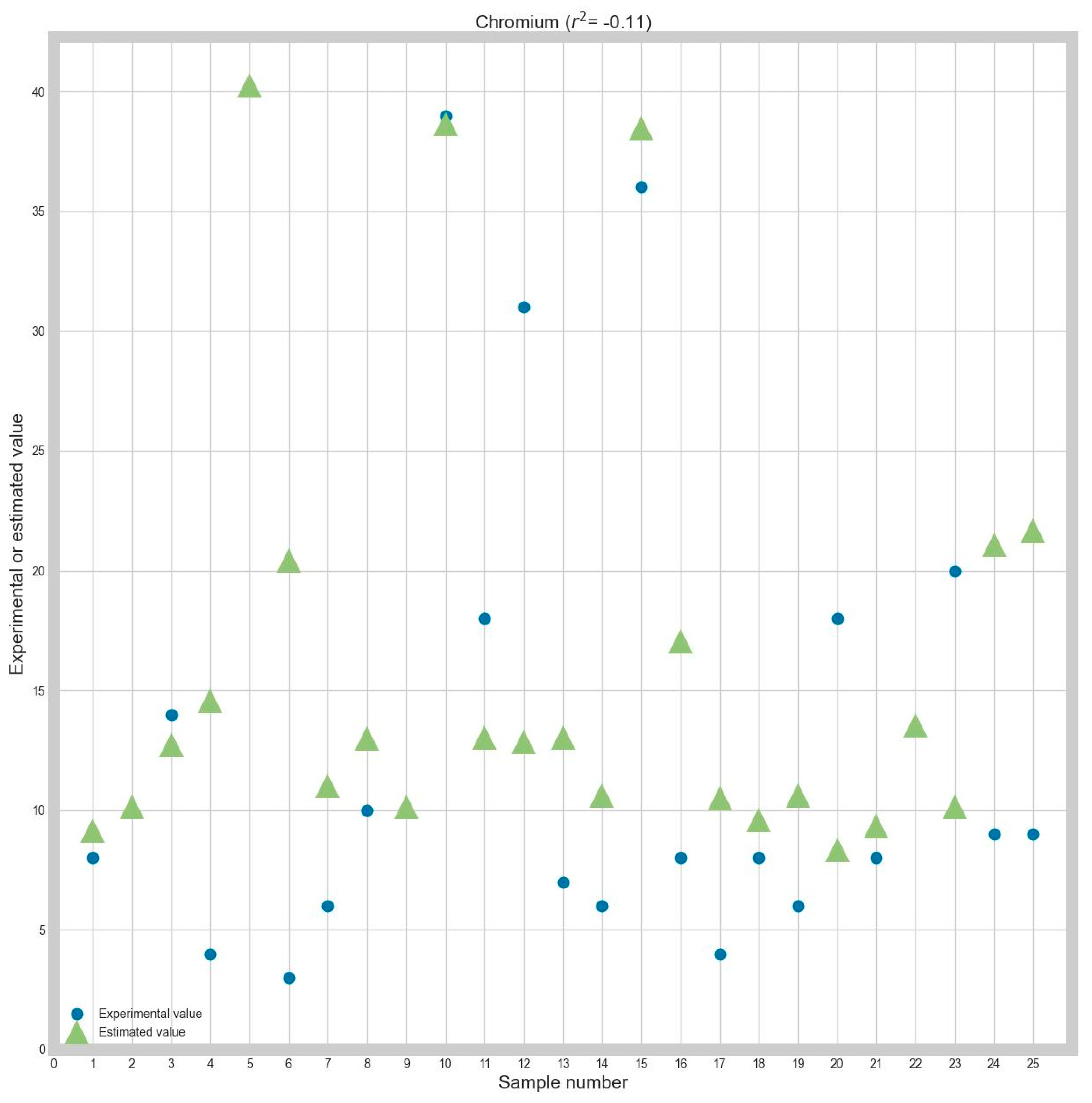
The obtained results for initial chromium are presented in

Table 7. Performance metrics values on the training and testing set for initial chromium.

Normalization Method	Criterion	Best Algorithm	Value on Training Set	Value on Testing Set
Z-score	MAE	Ada Boost	6.64	38.17
Z-score	RMSE	Ada Boost	8.38	110
Minmax	MAE	Ada Boost	6.57	38.17
Minmax	RMSE	Ada Boost	8.23	110.05

.

As can be seen in Table 7, the Ada Boost algorithm is the best option for the given training database is the Ada Boost algorithm.

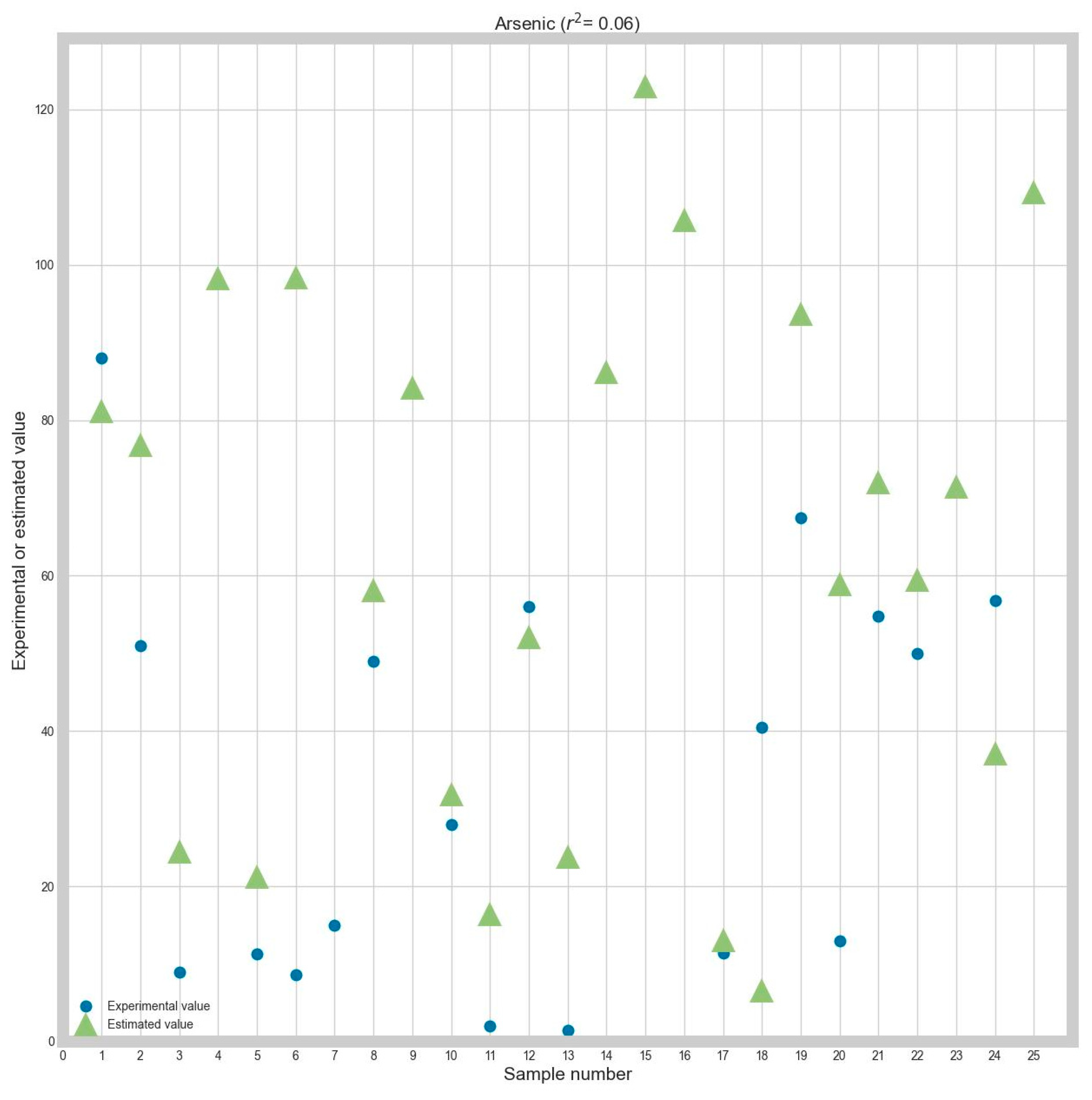
The obtained results for initial arsenic are presented in

Table 8. Performance metrics values on the training and testing set for initial arsenic.

Normalization Method	Criterion	Best Algorithm	Value on Training Set	Value on Testing Set
Z-score	MAE	Passive Aggressive	59.32	94.69
Z-score	RMSE	K-neighbors	89.73	144.49
Minmax	MAE	Huber	60.49	93.63
Minmax	RMSE	K-neighbors	89.73	144.49

.

The results from Table 8 show that minimizing RMSE is done best by the K-neighbors algorithm. The Passive Aggressive and Huber algorithms are better when minimizing the MAE.

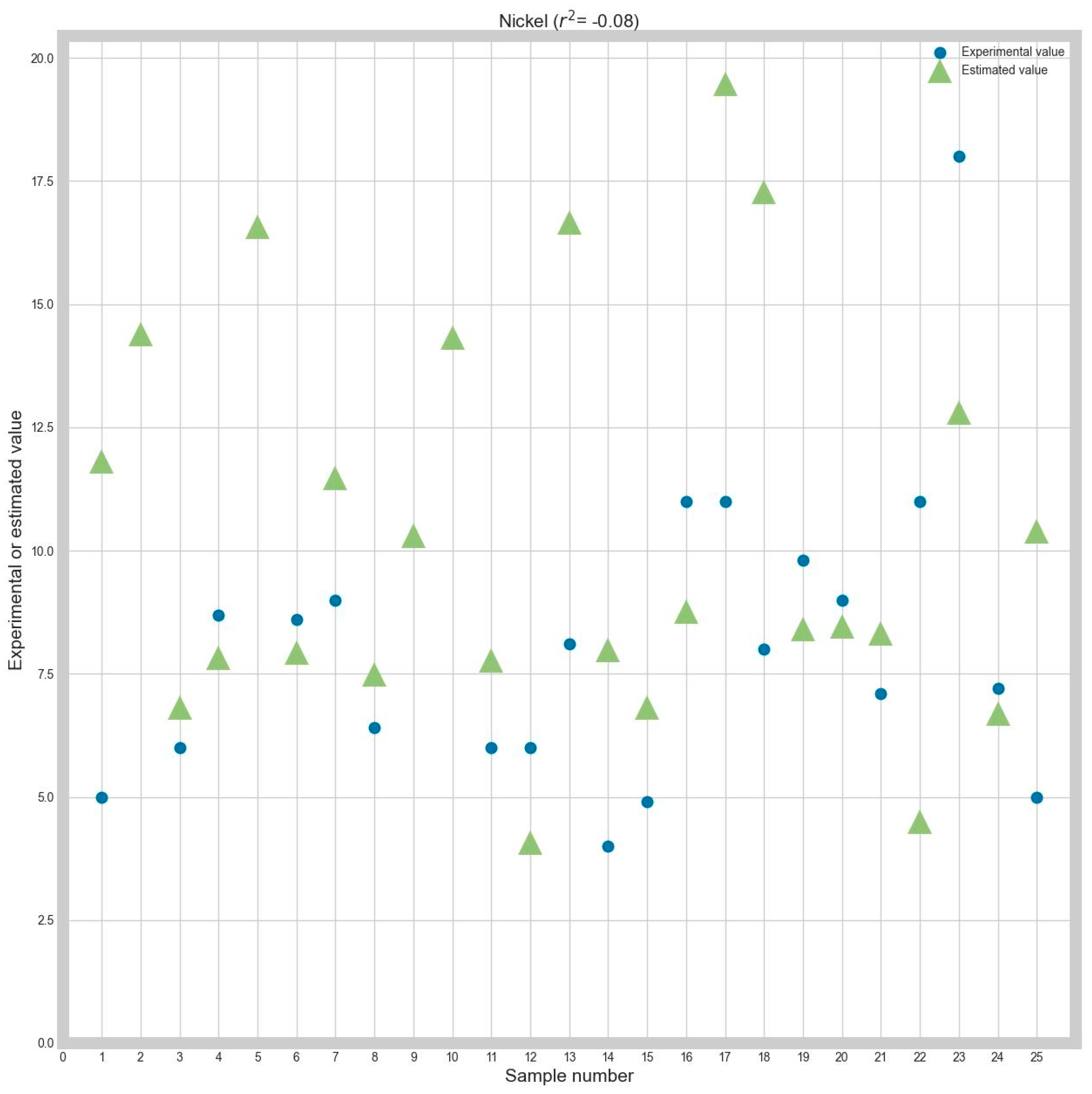
The obtained results for initial nickel are presented in

Table 9. Performance metrics values on the training and testing set for initial nickel.

Normalization Method	Criterion	Best Algorithm	Value on Training Set	Value on Testing Set
Z-score	MAE	Catboost	5.77	59.71
Z-score	RMSE	Catboost	8.25	198.35
Minmax	MAE	Catboost	5.77	59.71
Minmax	RMSE	Catboost	8.25	198.35

.

In Table 9, the Catboost algorithm is the best choice for the normalization methods and criteria considered.

Also, the following conclusions can be drawn by studying Table 2, Table 3, Table 4, Table 5, Table 6, Table 7, Table 8 and Table 9.

• The normalization method has little impact on the criterion values on both training and testing sets. This is to be expected because normalization is the same process. These methods were considered for the program because the Z-score normalization is sensitive to outliers, while the Minmax is not so sensitive. For the other training databases, it is possible that the choice of normalization method will bring significantly different results.
• The choice of the training criterion matters to the computed values. This is not only because of the way these criteria are computed but also because of the outlier sensitivity. MAE is not very sensitive to outliers, but RMSE is. If the training database has a lot of outliers, MAE may be a better choice than RMSE.
• In Table 6, Table 7, Table 8 and Table 9, the criterion values for the training set are much lower than for the testing set. There are many possible causes for this behavior. The authors believe that it is a sign of underfitting due to the small size of the training database.
• There are also cases where the values for the training dataset are higher than those for the testing dataset. Because the differences are not large, the authors cannot conclude that this is a case for overfitting. The training database size also rules out overfitting.

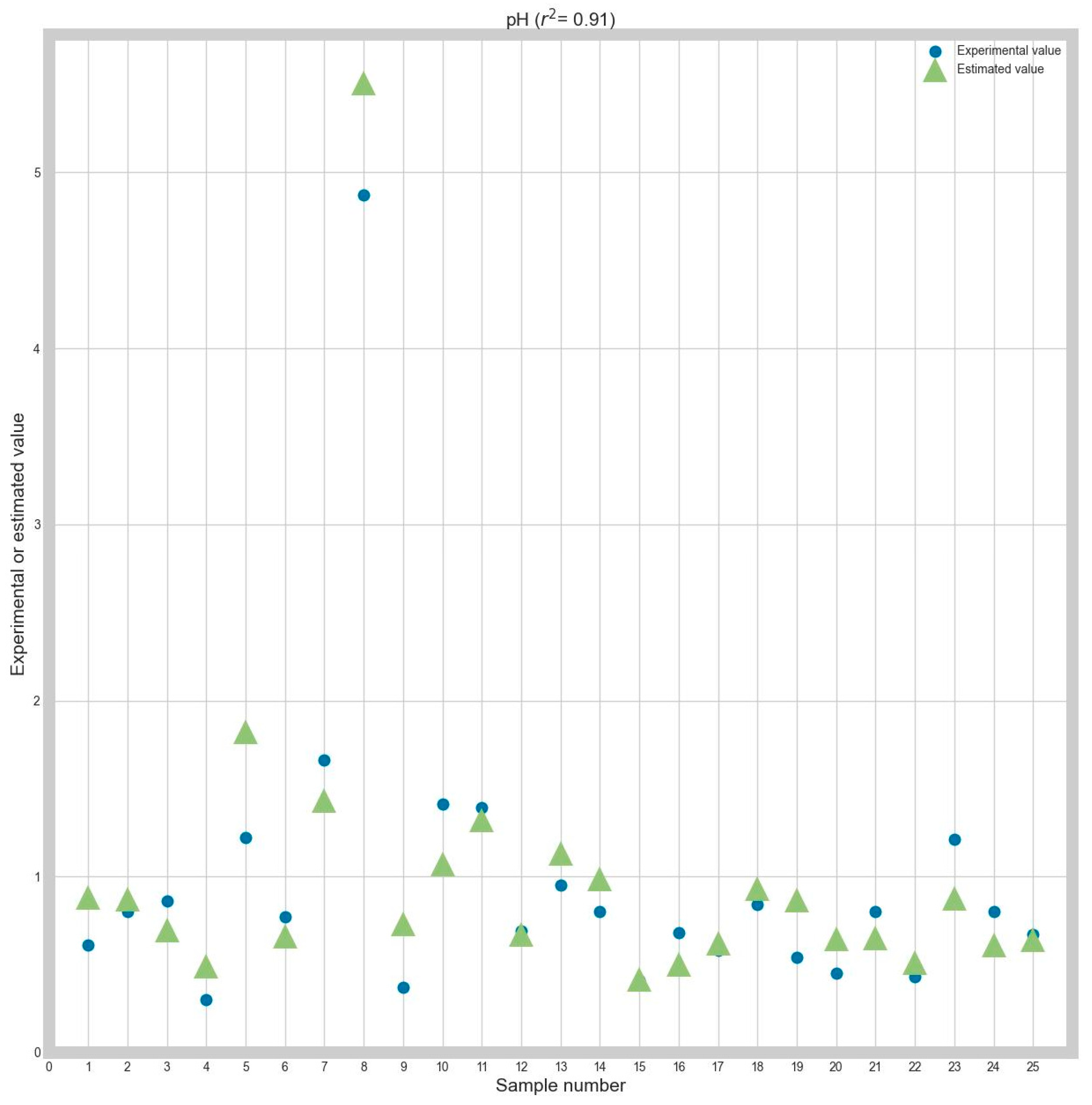
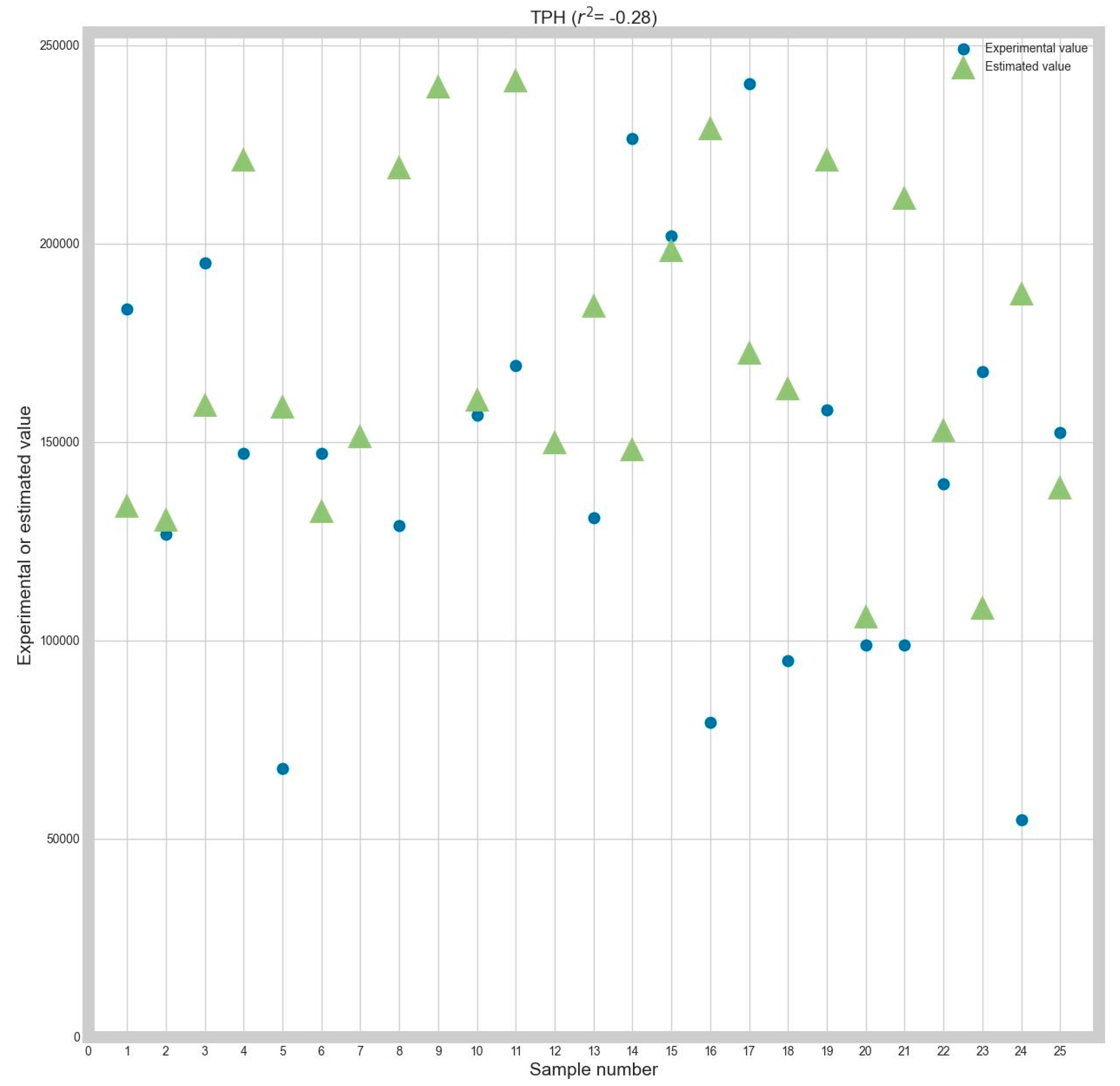
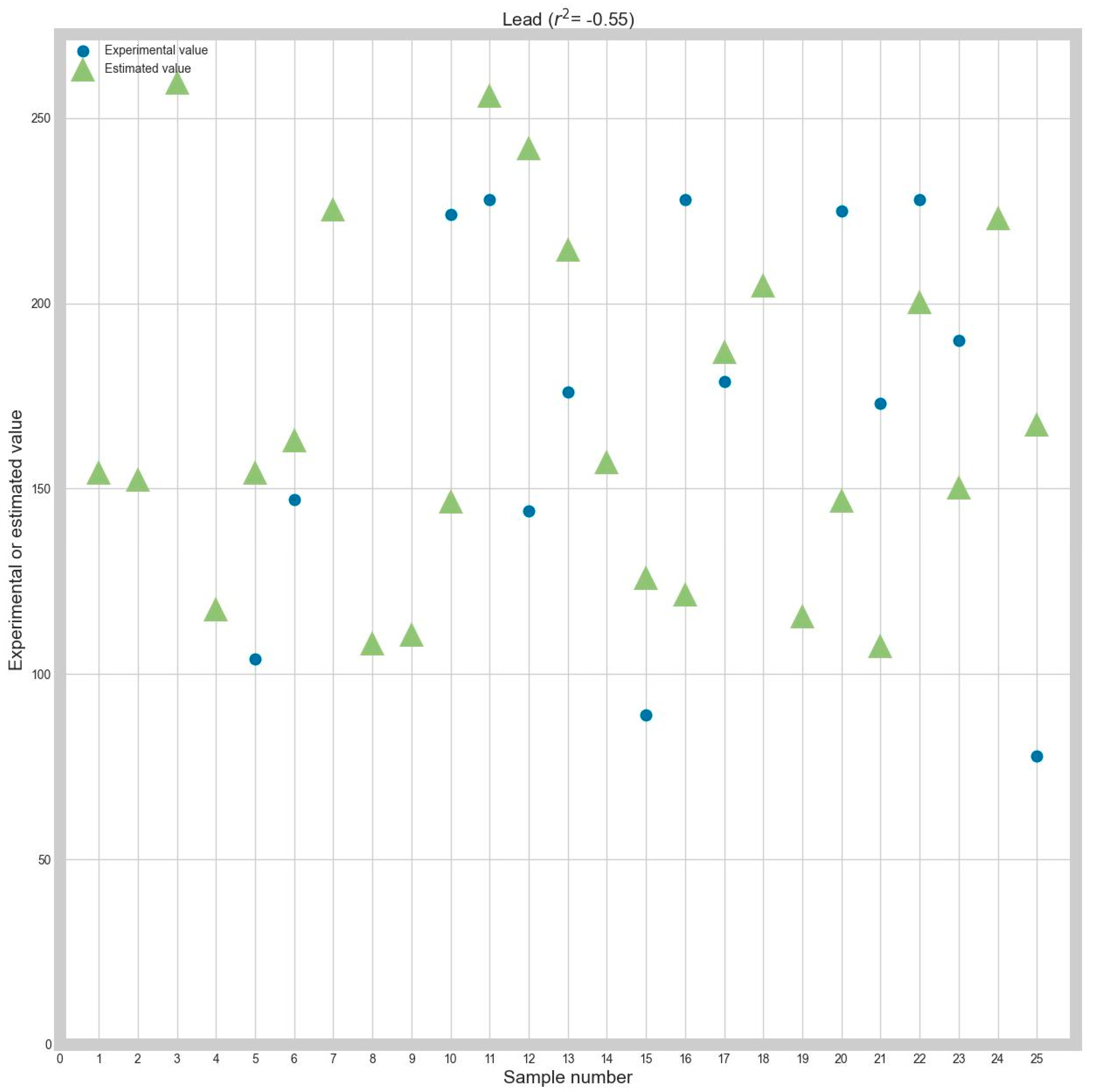
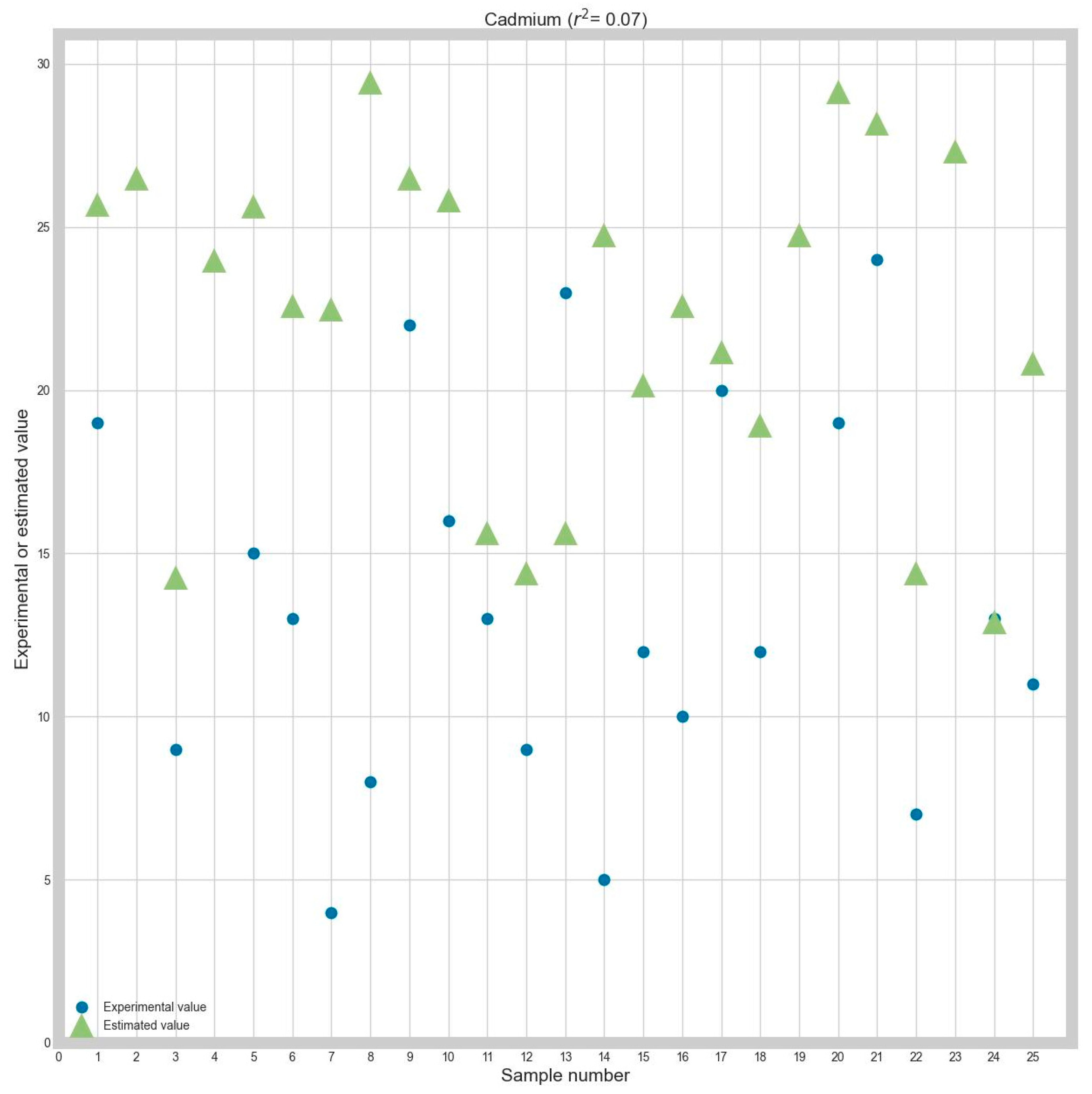
To make the obtained performance more suggestive, graphs between the determined and the real (ground truth) values will be presented. Because there are many combinations considered and for brevity reasons, graphs for only a part of the obtained results will be presented. More precisely, the graphs show the obtained and ground truth values for every response variable, using Z-score normalization and MAE as optimization criteria. Each graph will also contain the R² correlation coefficient for every prediction.

Also, to evaluate the prediction’s precision, each of the following graphs will contain the R² correlation coefficient between the real and the estimated data.

The R² correlation coefficient is a number between −1 and 1 that represents the proportion of variance of the response variable(s) that has been explained by the independent variable(s) in the model. It provides an indication of the goodness of the fit and, therefore, is a measure of how well the unseen samples are likely to be predicted by the model throughout the proportion of the explained variance [53].

The R² correlation was chosen because, in the authors’ opinion, it is a metric that is easier to interpret than MAE or RMSE. This is because MAE and RMSE do not have a ceiling, and it is much harder to assess the model’s accuracy only by looking at the MAE or RMSE values. However, R² is capped between −1 and 1, and the result interpretation is more straightforward: the higher the value, the higher the correlation.

A graphical comparison of the experimental and predicted pH values is presented in Figure 2.

A graphical comparison of the experimental and predicted TPH values is presented in Figure 3.

Graphical comparisons of the experimental and estimated lead, cadmium, copper, chromium, nickel, and arsenic concentrations are presented in Figure 4, Figure 5, Figure 6, Figure 7, Figure 8 and Figure 9.

The results of applying the presented method can be improved by increasing the amount of data in the training database. Thus, the presented method can be used to estimate the properties of acid tars.

The presented technique has its own limitations. The first limitation is that ML algorithms are very dependent on the provided training dataset. Ideally, the training dataset should be as large as possible (hundreds, thousands or even millions of records), and its records should be as correlated as possible. The more data and the more correlated the data from the dataset, the more reliable the ML algorithm that will process it.

The second limitation is in the choice of data preprocessing. The limitation is that there is no set algorithm to determine which type of preprocessing is appropriate for the specific problem. A mix of trial and error, statistical analysis, and experience are used in this case.

Another limitation is related to the candidate algorithms for ML modeling. In theory, any ML algorithm for a specific kind of problem can work due to the Garbage In, Garbage Out principle. In practice, only a couple of algorithms offer the best results. The limitation here is that there is no algorithm to determine which algorithm(s) are the best for a specific training database. Each algorithm has its own description, prerequisites, and strong and weak points, but testing them on a computer will let the programmer know if it can be applicable. This limitation is partially minimized by using AutoML technology.

Further research is required because the method presented therein can be improved. Here are a few of the improvements:

• Data preprocessing. Besides scaling, other preprocessing can be used: imputations, feature engineering, etc. It depends on the training data analysis.
• Choice of candidate algorithms. It is not mandatory to choose the algorithms presented in this paper. Depending on the characteristics of the training dataset, other algorithms may be tested as well. Some algorithms require dataset preprocessing, which must be applied before the training phase. Also, PyCaret can be programmed to accept machine learning algorithms other than its default.
• Choice of the hyperparameters for hyperparameter tuning. Each algorithm has a myriad of hyperparameters to choose from, and thus, a wide range of values can be tested. However, hyperparameter tuning will slightly improve the estimation power of an algorithm. It will not yield fantastic results from a badly chosen one. This part is facilitated by AutoML technology.
• Analyzing the possibility that there could be relationships between dependent variables. The PyCaret library does not allow multivariate regression using machine learning, but a future version of the program will make the appropriate changes.
• Analyzing the importance of each set of predictor data offers the user the possibility of eliminating the data that matters the least if they choose to.

Choice of the criteria to determine the best algorithm. MAE and RMSE are not the only existing criteria. Other criteria can be chosen.

This is the first such investigation in the open literature and therefore justifies the novelty of the current study.

5. Conclusions

Machine learning shows the potential to identify places where pollution is present in contaminated soil. In this study, the authors presented a methodology that uses machine learning to estimate the properties of the acid tars, knowing the place from which they were sampled and the depth of the taken samples.

This methodology uses AutoML techniques to determine the best algorithm and its hyperparameters for training and testing data.

In the next step, the above algorithms were chosen on a test set, with each acid tar property (pH, TPH, heavy metals, and As) being chosen as the response variable. The chosen performance criterion was R².

The results show that the correlation between the experimental data and the estimated data can be improved, mostly because of the low amount of data from the training database. Based on an exhaustive search performed by the authors, similar studies in estimating acid tar properties that consider machine learning applications remain unreported in the literature.

Furthermore, with supportive measures like open-data policies and data integration, AI/ML possesses the potential to revolutionize the practice of contaminated site remediation.