Article

Adaptive Graph Convolutional Network with Deep Sequence and Feature Correlation Learning for Porosity Prediction from Well-Logging Data

1
College of Software, China University of Petroleum, Qingdao 266555, China
2
College of Computer Science, China University of Petroleum, Qingdao 266555, China
*
Author to whom correspondence should be addressed.
Appl. Sci. 2025, 15(9), 4609; https://doi.org/10.3390/app15094609
Submission received: 18 March 2025 / Revised: 13 April 2025 / Accepted: 16 April 2025 / Published: 22 April 2025
(This article belongs to the Section Earth Sciences)

Abstract

:
Accurate porosity prediction is crucial for evaluating reservoir quality and potential productivity. Traditional laboratory experiments offer reliable porosity measurements but are time-consuming and computationally expensive. Recently, deep learning has been introduced for porosity prediction. However, most existing methods focus on either the relationships among features or deep sequences, neglecting the correlation between them. To better capture these correlations, we propose an adaptive graph convolutional network (GCN) with learning deep sequence and feature correlation graphs. The GCN is applied to well-logging data to capture non-Euclidean characteristics, extracting inherent spatiotemporal relationships. Furthermore, traditional GCNs rely on predefined graphs for feature aggregation, which can vary based on the thresholds for cosine similarity or covariance, potentially affecting accuracy and robustness. To tackle this issue, we introduced an adaptive mechanism for constructing deep sequence and feature correlation graphs, which eliminates the need for predefined thresholds and significantly enhances the accuracy and robustness of predictions. We demonstrated our method on well-logging datasets and comprehensively compared its performance with other deep learning models, showing its superiority in predicting porosity from well-logging data. This work offers geoscientists a more efficient and accurate analytical tool.

1. Introduction

In the petroleum industry, porosity [1] is a critical parameter for reservoir evaluation, as it measures the void spaces within rocks and is often correlated with reservoir quality [2]. Traditional methods of porosity measurement, such as core sampling and rock physical analysis, are costly and time-consuming. Additionally, incomplete logging data, due to the economic and physical limitations of tools, as well as the complex nonlinear relationships between geological factors and logging parameters, pose significant challenges. Empirical equations often fail in different regions, prompting a shift towards nonlinear multivariate regression and models incorporating geological and mechanical properties [3]. However, the heterogeneous variations and nonlinear correlations of subsurface structures often result in unsatisfactory predictions.
Machine learning algorithms have become an essential tool for predicting reservoir parameters, effectively addressing the nonlinear challenges faced by traditional methods [4]. These approaches enhance the accuracy and efficiency of porosity prediction by integrating logging data with geological information and optimizing exploration and development strategies in the petroleum industry. Distinguished from conventional techniques [5] that depend on expert analysis of log data, machine learning, notably deep learning, autonomously extracts features from data, adjusts to a range of geological settings, and demonstrates enhanced adaptability [6]. Among the widely recognized deep learning approaches are convolutional neural networks (CNNs) [7,8], recurrent neural networks (RNNs) [9,10], long short-term memory (LSTM) networks [11], and gated recurrent units (GRUs) [12] and their variants [13,14,15]. For example, Chen et al. [16] innovatively developed a multi-layer LSTM (MLSTM) method based on the traditional LSTM model for porosity prediction, which was tested on three wells in southern China. The results showed that MLSTM method exhibited superior robustness and accuracy in deep sequence prediction compared to GRUs and RNNs.
Different network models exhibit unique effectiveness when processing various types of data. RNNs and LSTM have the capability to retain previous information. At the same time, CNNs can automatically extract features that help capture relationships between variables, thereby enhancing predictive performance. However, a single model is typically only able to capture specific types of features, such as sequential or spatial characteristics. Research has shown that uncovering the correlations between deep sequences and features in logging curves can improve the accuracy of predictions [17]. Although CNNs excel at processing images and data with strong spatial correlations, they fall short in capturing the potential spatial correlations between different logging curves [18]. Graph neural networks (GNNs), on the other hand, can effectively handle non-Euclidean data by uncovering hidden spatial dependencies through local connectivity and permutation invariance [19]. GNNs have been thoroughly validated for capturing sequence and feature correlations, yet their primary applications are still concentrated in specific domains such as traffic flow and offshore wind speed prediction [20,21,22,23,24]. To reveal correlations within logging data, an increasing number of studies are employing undirected graphs, where the graph vertices represent data vectors and the edges represent the similarities or affinities of logging data. Graph convolutional networks (GCNs) excel at handling undirected graphs by incorporating their underlying topological structure [25]. GCNs estimate porosity through the use of multiple sequential spectral graph convolutions. In each stage, the model carries out a dual process: initially, it consolidates analogous data points according to an established graph topology, followed by a transformation that elevates the data into an expanded dimensional realm, thereby enriching the feature set. Deep sequence correlation graphs are undirected graphs constructed in the spatial domain, where each node denotes a collection of features at a given time point. By handling graphs of deep sequence correlations, GCNs can synthesize various features from multiple time points, thereby accounting for profound sequence dependencies in the prediction of porosity. Feature correlation graphs are undirected graphs constructed within feature channels, where each node corresponds to an individual depth-wise sequence attribute. By processing these graphs, GCNs are able to combine analogous features, enabling the model to capture and incorporate feature correlations for more accurate porosity prediction [26].
In summary, our proposed model has proven to be effective for porosity prediction. For instance, Feng et al. [27] designed an adaptive spatio-temporal graph neural network (ASTGNN), which effectively captures the spatial and temporal dependencies among available logging measurements by integrating GCNs and temporal convolutional networks (TCNs). Their experimental results validated the method’s accuracy and superior performance in both univariate and multivariate regression logging predictions on a Norwegian oilfield dataset and China’s Daqing dataset.
However, enhancing the accuracy and robustness of the model requires overcoming two key issues. First, existing GCNs depend on a single graph type, be it a deep sequence correlation graph or a feature correlation graph, which restricts their capacity to capture the full spectrum of sequence and feature correlations in logging data [27]. Second, traditional GCNs heavily rely on predefined graphs for feature aggregation, where the graph topology can vary based on the thresholds of cosine similarity or covariance, potentially affecting the precision and stability of the predictions [28,29].
To address these issues, this study concurrently considers two key factors for predicting porosity from logging curves: the correlation between deep sequences, and the correlation between features. We input the deep sequence correlation graph into GCNs to capture non-Euclidean features in logging data, extract inherent spatiotemporal relationships within formation data, and thereby construct dependency relationships within complex geological structures. The input features are physical quantities measured by logging tools, used to derive the physical properties of subsurface rocks for interpreting the structure and characteristics of the formation. The feature correlation graph, an undirected structure formed within feature channels, assigns each node to a distinct time series attribute. The GCNs processing the feature correlation graph can aggregate similar features to account for the feature correlation in porosity prediction. Taking both factors into account offers significant advantages for handling logging tasks with complex geological structures and intricate dependencies among different physical quantities. Furthermore, to overcome the limitations of predefined graphs, we use an adaptive mechanism that can automatically construct temporal correlation graphs and feature correlation graphs without setting thresholds. This mechanism enables the predictive model to dynamically learn the graph structure during training, substantially boosting the accuracy and robustness of its predictions. Finally, to prevent redundancy in processing both deep sequence correlation graphs and feature correlation graphs, we employ an attention-based selection method to pinpoint and extract the key features emerging from the attention graph convolution operations and dynamically adjust their contributions to porosity prediction, thus improving the model’s accuracy and robustness.

2. Methods

In this section, we introduce the proposed adaptive graph convolutional network with deep sequence and feature correlation graphs. Figure 1 presents the computational structure of the proposed adaptive graph convolution operation, which includes feature extraction and selection, adaptive construction of graphs, spectral graph convolution operations for temporal correlation graphs and feature correlation graphs, and porosity prediction based on multi-head attention. First, we describe how to adaptively construct deep sequence and feature correlation graphs, followed by an introduction to spectral graph convolution operations suitable for processing the topologies of deep sequence and feature correlation graphs, and finally, we present the multi-head attention mechanism for eliminating redundant information.

2.1. Adaptive Construction of Deep Sequence and Feature Correlation Graphs

Two spectrogram convolution operations were initialized from deep sequence correlation and feature correlation graphs. To construct the feature space, we extracted features from the well-logging data using a sliding window with a length of S and a step size of 1. The i-th sampling is denoted as X i R S × F , where S represents the moving window length and F denotes the number of features extracted. Typically, deep correlation and feature covariance graphs are initialized by calculating the cosine similarity matrix C i R S × S and the covariance matrix E i R F × F . These two matrices can be computed from X i . The matrix element c s , s ( i ) of C i can be obtained using Equation (1), where x s ( i ) refers to the s-th column vector associated with the i-th group of extracted features.
c s , s ( i ) = x s ( i ) · x s ( i ) / x s ( i ) x s ( i ) , s = 1 , , S ,
The matrix element e f , f ( i ) of E i can be derived from Equation (2), where x f ( i ) represents the f-th row vector of the i-th extracted feature; E [ · ] denotes the expectation of a vector.
e f , f ( i ) = E x f ( i ) E x f ( i ) x f ( i ) E x f ( i ) , f = 1 , , S ,
The cosine similarity matrix C i can be used to derive the depth sequence correlation adjacency matrix A d R S × S through Equation (3), where a s , s represents an element of the adjacency matrix A d . The value of this matrix is determined by the threshold θ . If a s , s = 1 , an edge exists between nodes s and s in the deep sequence graph G d , whereas if a s , s = 0 , no edge is present between them in G d . If there is no edge, the two nodes are not correlated along the depth sequence. If there is an edge, this means the two nodes are correlated along the depth sequence.
a s , s = 1 , c s , s ( i ) θ 0 , c s , s ( i ) < θ ,
The covariance matrix E i can be used to derive a feature correlation adjacency matrix A f R F × F through Equation (4), where a f , f represents an element of the adjacency matrix A f . If two features are correlated by E i , a f , f is set to 1; otherwise, it is set to 0. When a f , f = 1 , an edge exists between nodes f and f in the depth sequence correlation graph G f , indicating feature correlation. If a f , f = 0 , no edge exists between the nodes, signifying that the features are uncorrelated.
a f , f = 1 , e f , f ( i ) > 0 0 , e f , f ( i ) 0 ,
The topological structure of the graphs preconstructed through the cosine similarity matrix C i and the covariance matrix E i may vary due to the predefined threshold θ , which may affect the precision and reliability of porosity prediction. (A quantitative analysis of the graph determinacy for these two preconstruction methods is provided in Appendix A). To tackle this, we implemented an adaptive mechanism for constructing deep sequence correlation graphs and feature correlation graphs without preset thresholds, enabling the model to dynamically learn the graph structure during training. The core idea of constructing the deep sequence correlation graph G d and the feature correlation graph G f lies in creating corresponding graph adjacency matrices A d and A f . Using a self-attention mechanism [30] to build the graph allows for the creation of an attention adjacency matrix, capturing the significance of the logging data. In the aggregation phase, the model relies on the attention adjacency matrix’s weights over the traditional scaled adjacency matrix’s coefficients, ensuring the prioritization of relevant and significant data. Furthermore, the self-attention mechanism can generate values for A d and A f that are between 0 and 1, which aids in avoiding gradient explosion and vanishing issues when dealing with automatically constructed graphs.
The deep sequence adjacency matrix A d derived from the attention mechanism is expressed by Equation (5), where SoftMax is an exponential normalization function that transforms input values into output probability distributions; the hyperbolic tangent function, or Tanh, serves as the activation function, and W d , 1 and W d , 2 represent the learnable weight matrices within the attention mechanism.
A d = SoftMax ( W d , 2 · tanh ( W d , 1 · X i T ) ) ,
Similarly, the feature adjacency matrix A f derived from the attention mechanism is given by Equation (6), with W f , 1 and W f , 2 representing the learnable weight matrices within the attention mechanism.
A f = SoftMax ( W f , 2 · tanh ( W f , 1 · X i ) ) ,
The attention adjacency matrices A d and A f are used to construct the deep sequence correlation graph G d and the feature correlation graph G f , respectively. These adjacency matrices are then utilized for spectral graph convolution operations, which are subsequently applied to the prediction of logging porosity. Part (B) of Figure 1 depicts the complete process of adaptively constructing the deep sequence correlation graph and the feature correlation graph.

2.2. Spectral Graph Convolution

After constructing the deep sequence correlation graph G d and the feature correlation graph G f , we process the topological structures of both graphs G d and G f separately using two spectral graph convolution operations. Equation (6) describes the spectral graph convolution operations, where g d denotes the graph convolution kernel from the deep sequence correlation graph G d , and g f denotes the graph convolution kernel from the feature correlation graph G f ; F represents the graph Fourier transform, and F 1 represents the inverse graph Fourier transform.
g * G d , G f X i = F F g d F X i , F 1 F g f F X i T ,
To facilitate understanding of Equation (7), the spectral graph convolution operations performed on G d and G f can be rewritten in terms of the eigendecomposition of a deep sequence Laplacian matrix L d and a feature Laplacian matrix L f . The definitions of the Laplacian matrices L d and L f are given by Equation (8) and Equation (9), respectively.
L d = I d D d 1 / 2 A d D d 1 / 2 ,
L f = I f D f 1 / 2 A f D f 1 / 2 ,
where I d R S × S and I f R F × F are identity matrices. D d and D f are diagonal matrices representing the node degrees in G d and G f , respectively. Since the Laplacian matrices L d and L f are real symmetric matrices, their eigendecomposition can be expressed as in Equations (10) and (11).
L d = Q d d Q d 1 = Q d d Q d T ,
L f = Q f f Q f 1 = Q f f Q f T ,
where Q d and Q f represent the eigenvectors of L d and L f , respectively; and d and f represent the arrays of eigenvalues of L d and L f , respectively. The spectral graph convolution operations performed on G d and G f , rewritten in the form of eigendecomposition of the Laplacian matrices, can be expressed as Equation (12).
g * G d , G f X i = Q d Q d T g d Q d T X i , Q f Q f T g f X i Q f T ,
Equation (12) can also be expressed as Equation (13), where θ d represents the learnable parameters for the graph convolution kernel g d , and θ f represents those for g f .
g * G d , G f X i = Q d g d , θ d ( Λ d ) Q d T X i , Q f g f , θ f ( Λ f ) Q f T X i T ,
By substituting Equations (10) and (11) into Equation (13), we can derive Equation (14).
g * G d , G f X i = g d , θ d ( L d ) X i , g f , θ f ( L f ) X i T ,
Since solving Equation (14) is computationally expensive, it is widely accepted to use the first-order Chebyshev polynomial approximation technique for spectral convolution operations [31]. Equation (15) provides the first-order Chebyshev polynomial approximation of Equation (14). Here, N = 1 represents the first-order approximation, and T N ( · ) is the Nth-order Chebyshev polynomial.
g * G d , G f X i = n = 1 N θ d , N T N ( L d ) X i , n = 1 N θ f , N T N ( L f ) X i T ,
Substituting Equations (8) and (9) into Equation (15) yields Equation (16). Here, Θ d R F × F represents the parameter matrix for the graph filter g d , while Θ f R S × S represents the parameter matrix for the graph filter g f .
g * G d , G f X i = A d X i Θ d , A f X i T Θ f ,
To augment the efficacy of the spectral graph convolutions, Equation (16) is augmented with a bias term and an activation function. The ensuing equation is portrayed as Equation (17), wherein b d signifies the deep sequence bias vector, b f signifies the feature bias vector, and σ signifies the activation function.
g * G d , G f X i = σ A d X i Θ d + b d , A f X i T Θ f + b f ,
Part (C) of Figure 1 illustrates the spectral graph convolution operations for the deep sequence correlation graph and the feature correlation graph. In this operation, the topological structure of the constructed graphs is utilized to aggregate the deep sequence and feature information based on their neighbors at each corresponding node, capturing the correlations between logging data.

2.3. Porosity Prediction Based on Multi-Head Attention Mechanism

The deep sequence correlation graph G d is generated from the sampled data X i T , and the feature correlation graph G f is generated from the sampled data X i . Using the same sampled data X i to generate G d and G f for spectral graph convolution operations may lead to redundancy and overlapping information. The tensor obtained after spectral graph convolution operations is defined as B i , as shown in Equation (18). Employing the raw result tensor B i directly in porosity estimation might diminish the predictive accuracy.
B i : = g * G d , G f X i = σ A d X i Θ d + b d , A f X i T Θ f + b f ,
Therefore, we employ a multi-head attention mechanism to extract the most pertinent information from the result tensor B i for prediction. This allows us to select the most relevant information from the logging data for prediction and project the result tensor B i into a higher-dimensional space. Thus, this minimizes redundancy and overlaps in the high-dimensional space. During this phase, the resulting tensor B i undergoes multiple parallel linear transformations to generate diverse representations of the input data, as depicted in Equation (19).
Q i ( h ) , K i ( h ) , V i ( h ) = B i · W Q ( h ) , W K ( h ) , W V ( h ) ,
where W Q ( h ) , W K ( h ) , and W V ( h ) represent the weight matrices for obtaining the corresponding higher-dimensional queries Q i ( h ) , keys K i ( h ) , and values V i ( h ) of the hth head. The final output result H i ( h ) of the ith sampled feature in the hth head can be given by Equation (20), with d being the weight matrix dimension.
H i ( h ) = SoftMax Q i ( h ) · K i ( h ) / d V i ( h ) ,
Next, the outputs H i ( h ) from each head in the multi-head attention mechanism can be concatenated as depicted in Equation (21).
MultiHead ( Q , K , V ) i = Concat SoftMax Q i ( h ) · K i ( h ) / d V i ( h ) ,
Ultimately, the output from the multi-head attention mechanism MultiHead ( Q , K , V ) i is flattened and fed into a fully connected(FC) layer to determine the final porosity estimate, as expressed in Equation (22). Here, W denotes the weight matrix of the FC layer, b represents the bias vector within the layer, and y ^ i signifies the resulting forecast.
y ^ i = σ W · F C MultiHead ( Q , K , V ) i + b ,
The loss function l used for training can be represented as Equation (23). To avoid overfitting, L 2 regularization terms are appended to the parameter matrices Θ d of the graph convolution kernel g d and Θ f of the graph convolution kernel g f .
l = 1 Ω i i = 1 Ω i y i y ^ i 2 + λ Θ d 2 2 + Θ f 2 2 ,
where λ signifies the regularization coefficient for the L 2 penalty term, Ω i denotes the count of windows, and y i corresponds to the actual outcome.
Part (D) of Figure 1 depicts the porosity estimation utilizing the multi-head attention framework. Within this concluding stage, the multi-head attention system identifies and prioritizes the most pertinent data for forecasting, simultaneously discarding irrelevant and repeated details.

3. Experimental Data Analysis

In this paper, the sample data were real data of the Tarim Oilfield in Western China. A cumulative total of 2800 datasets were assembled, encompassing various logging parameters such as shared photoelectric index (PE), density (DEN), sonic time difference (AC), gamma (GR), 2.5 m bottom gradient resistivity (R25), neutron (CNL), and high-resolution array induced polarization resistivity (M2R1). These parameters constitute fundamental physical measurements obtained from logging instruments. Utilized to ascertain the properties of underground formations, these data facilitated the analysis of stratigraphic composition and attributes. The collected porosity data mainly stemmed from laboratory measurements and interpretations derived from well-logging data. Laboratory measurements were conducted through lithological sampling methods, starting with the use of a core drill to perform coring operations and obtain core samples. These samples were then sent to the laboratory for porosity analysis. Well-logging interpretation used techniques such as natural gamma logging, neutron logging, and sonic logging to measure the physical properties of strata and model the physical characteristics of subsurface rocks. To ensure data accuracy and reliability, we corrected and processed the collected logging data. Finally, these logging data were integrated with established physical property models to interpret the structure and characteristics of the strata.
PE describes a material’s ability to absorb photons during the photoelectric effect [32]. It includes the mass photoelectric absorption cross-section index and the volume photoelectric absorption cross-section index of rocks, representing the average photoelectric absorption cross-section of photon interactions with an electron in the rock. Through the photoelectric absorption cross-section index, it is possible to predict and assess the porosity of rocks. The DEN logging technique estimates the density of geological formations by quantifying radiation absorption [33]. The DEN logging apparatus comprised a radiation emitter and corresponding detectors, calculating density by measuring changes in radiation intensity after passing through the formation, thereby determining the physical properties of the rock layers. AC logging evaluated the porosity of rock formations by measuring the propagation speed of sound waves in the rock formations [34]. The logging tool’s acoustic sensor emits sound waves, recording their travel time. Using these data and the established sound velocity, the formation’s acoustic transit time difference was determined. GR logging is a method for evaluating rock properties by measuring the natural gamma radiation intensity of rock layers [35]. Since rocks contain varying amounts of radioactive elements that continuously emit radiation, these measurements allow us to delineate the geological profile of a borehole, determine the shale content in sandstone and shale profiles, and qualitatively assess the porosity of rock layers. R25 reflects the resistivity characteristics of fluids in a formation. Its measurement is based on the resistivity of the rock, and by analyzing the resistivity differences between the fluids and the rock matrix, the formation’s porosity can be estimated. CNL Logging measures the absorption of fast and thermal neutrons by rock formations, to reflect the hydrogen content, indirectly assessing the porosity of the formation [36]. A high hydrogen content usually indicates higher porosity, as hydrogen is a major component of fluids (such as water or hydrocarbons) in the rock, which typically occupy the pore spaces. M2R1 logging uses multiple receiver and transmitter combinations to measure the resistivity of formations at different radial depths, providing high-resolution resistivity data that, when combined with geological and geophysical models, can predict the porosity of formations.
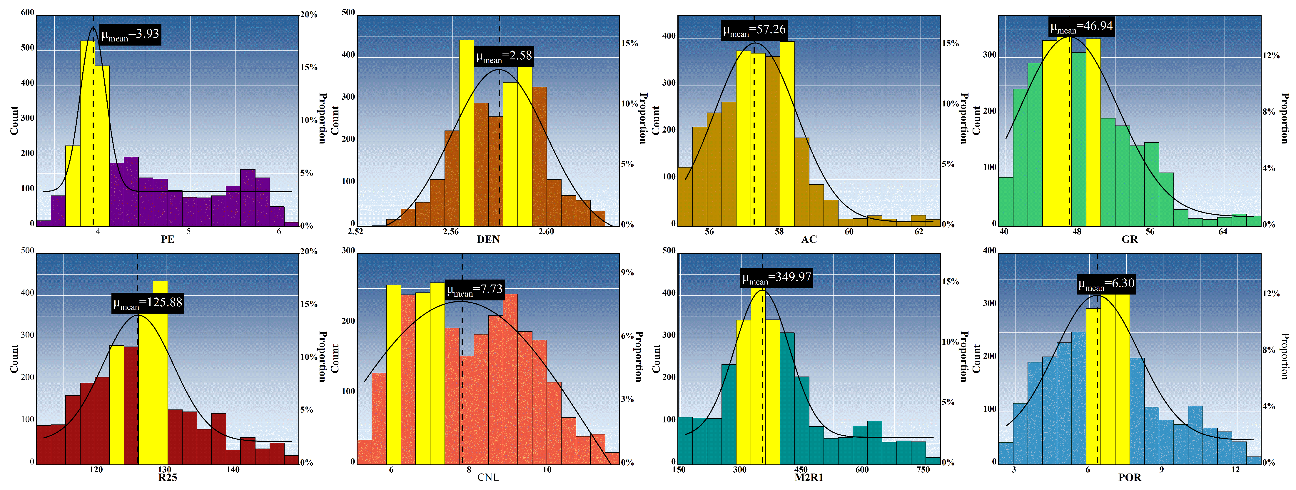
Next, we analyzed the distribution of the raw data through statistical analysis. Table 1 shows the logging parameters and porosity statistical analysis. These logging parameters were obtained through logging tools, but accurate porosity values needed to be obtained through indoor experiments and coring. The main task of this article was to test the porosity prediction algorithm based on indoor porosity measurement data. Figure 2 and Figure 3 present distribution histograms and violin plots of the data, respectively, revealing the normal distribution characteristics of the data. This distribution is crucial for regression prediction, as it lays a scientific foundation for parameter estimation and statistical inference, and ensures the reliability and effectiveness of regression analysis. Following a normal distribution of data allows us to more accurately identify the correlation between independent and dependent variables, and predict future development trends.
We allocated the dataset into training and testing subsets with a ratio of 6:4, ensuring ample data for model training to capture features and trends. This method also facilitated assessing the model’s predictive performance on unseen test data.

4. Analysis of Prediction Results

To evaluate the efficacy of our adaptive graph convolutional network for deep sequence and feature correlation graphs (ATF-GCN), we conducted ablation and comparative experiments with the methodologies detailed in Table 2.
Table 3 details the hyperparameter configurations for the methods mentioned in Table 2. Our proposed model aims to strike a balance between capturing data patterns and controlling complexity, to avoid overfitting. To this end, we set three graph convolutional layers and the number of heads in the attention mechanism is set to two. The window size (S), a critical hyperparameter, substantially influences both predictive accuracy and processing duration. We determined the ideal window size by conducting a grid search from 5 to 50, to balance between the enhanced prediction accuracy with larger windows and the reduced computational expense associated with smaller windows. Setting the window size to 12 achieved an optimal prediction performance, without significantly increasing the computational cost. Additionally, we chose ReLU as the activation function, to leverage its efficiency and effectiveness in capturing non-linear relationships. The learning rate was set to a common starting value of 1 × 10 4 , which helped the model to converge stably and prevented overly rapid parameter updates. For the optimizer, we selected Adam, which effectively updates model parameters through its adaptive learning rate mechanism. At the same time, we set the dropout rate to 0.3 to achieve a moderate regularization effect, enhancing the model’s generalization ability without harming the learning performance due to an excessively high dropout rate. To ensure a fair comparison between models, all models in the ablation experiment adopted a unified set of hyperparameters. This consistency ensured that any performance differences could be attributed to the model architecture itself.
The BiGRU model was configured with 128 GRU units per layer. The choice of 128 units struck a balance between model capacity and the potential for overfitting. The learning rate was set to 0.001. We configured a dropout rate of 0.3 and opted for the ReLU activation function, aligning with the ablation experiment model ensemble that controlled the experimental variables. Since BiLSTM and BiGRU are analogous in deep learning, the parameter settings were consistent, ensuring that the experimental variables remained manageable.
Table 4 presents the four evaluation metrics for the deep learning model: RMSE, R 2 , MAE, and MAPE. RMSE measures the difference between a model’s predicted and actual values by squaring the error, averaging, and then taking the square root. A smaller RMSE indicates a better model fit. The formula for RMSE is shown in Equation (24). R 2 evaluates how well a model explains the variance in the dependent variable, with values closer to 1 indicating better explanation. Equation (25) provides the formula for R 2 . MAE is the mean absolute error between the predicted and actual values, being less sensitive to outliers and reflecting overall model fit. The formula for MAE is given in Equation (26). MAPE measures the average relative error; a smaller MAPE indicates a better fit. Equation (27) shows the MAPE formula.
RMSE = 1 N i = 1 N P O R i P O R i ^ 2 ,
R 2 = 1 i = 1 N P O R i P O R i ^ 2 / i = 1 N P O R i P O R i ¯ 2 ,
MAE = 1 N i = 1 N P O R i ^ P O R i ,
MAPE = 1 N i = 1 N P O R i ^ P O R i P O R i × 100 % ,
where P O R i is the predicted porosity value, P O R i ^ is the actual porosity value, P O R i ¯ is the average porosity, and N is the number of sample points.
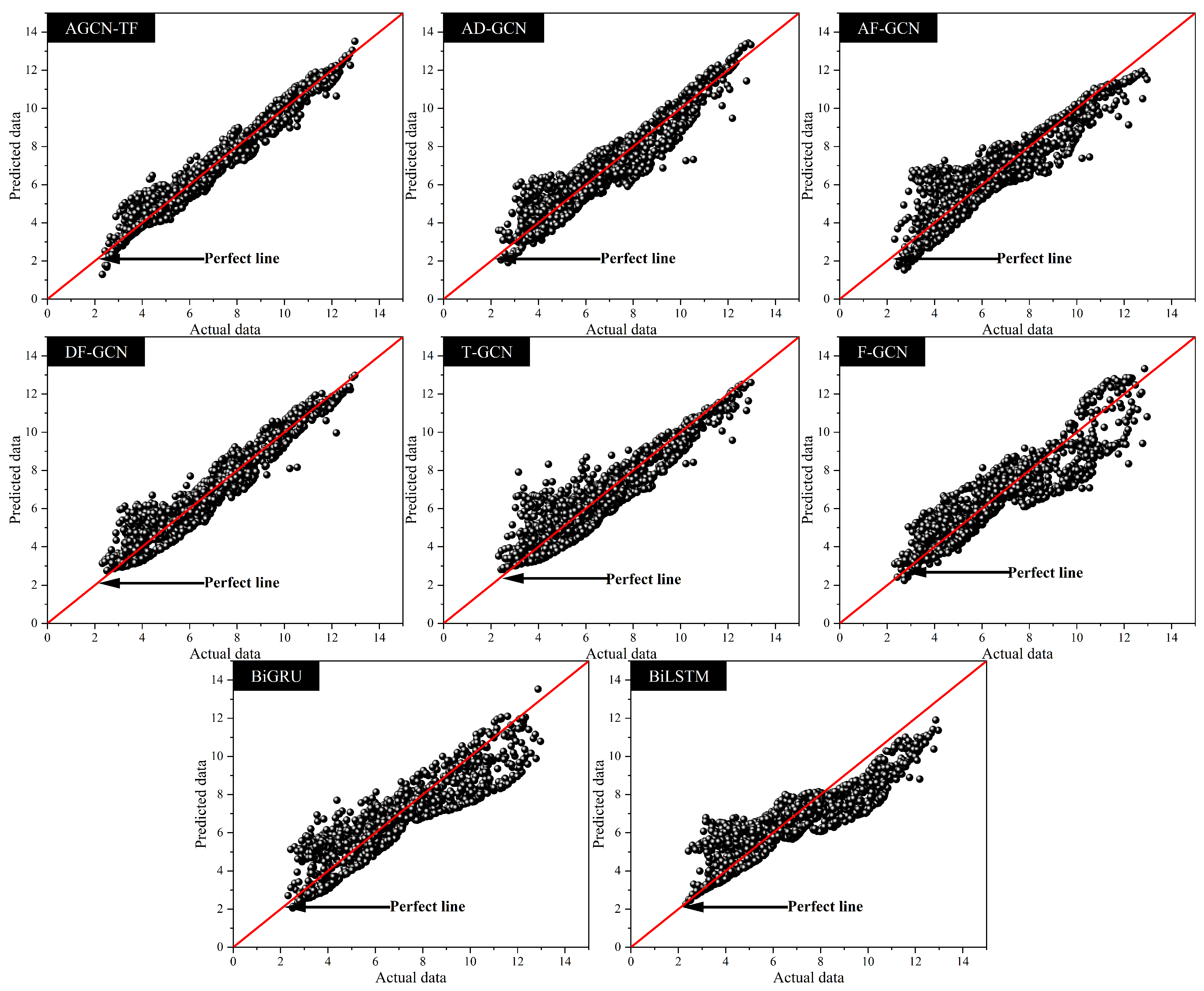
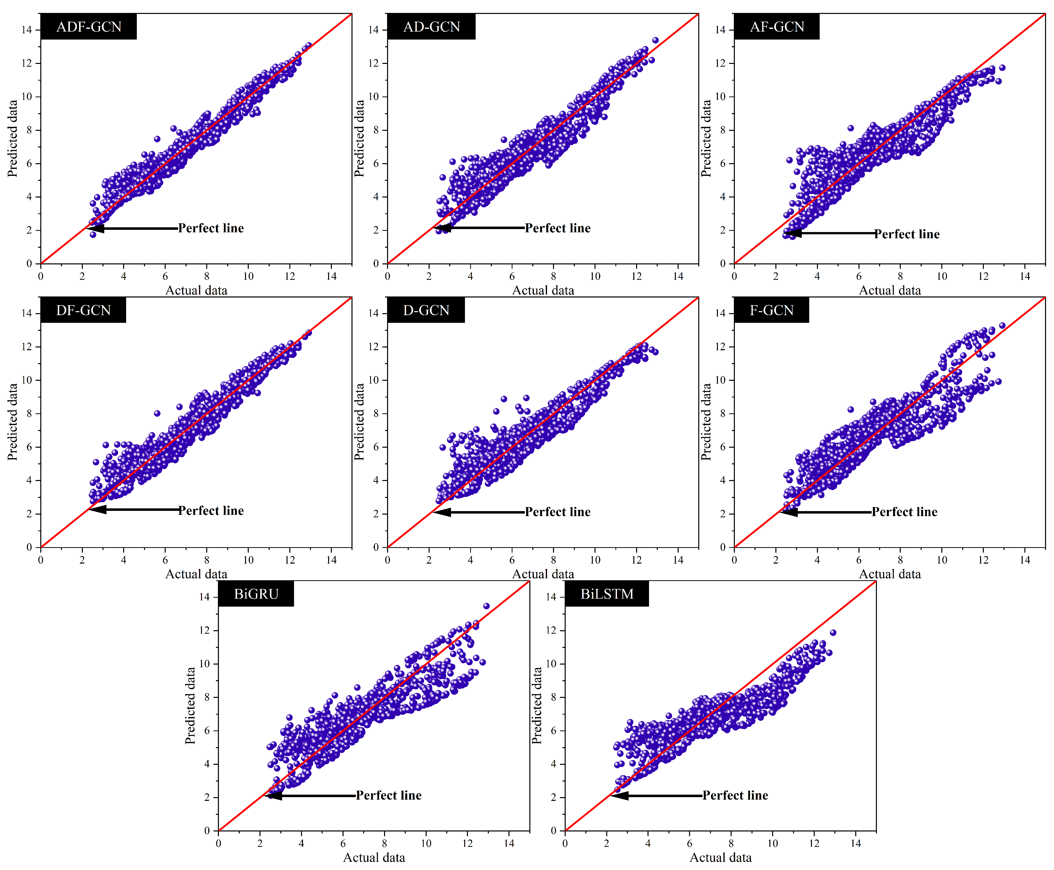
Figure 4 and Figure 5 display scatter plots of the true versus predicted values for the training and test sets, respectively. From the data in the figure, it can be seen that the ADF-GCN model ( R 2 = 0.9509 ) has the closest scatter to the diagonal line, indicating that the model’s predictions were closest to the true values on the training set, and the overall prediction accuracy was the highest. The scatter of the DF-GCN model ( R 2 = 0.9235 ) is closer to the diagonal line than the other ablation model ensemble, indicating that the prediction accuracy of the model that considered both the deep sequence and the feature-related graph was higher. The model that took into account both the deep sequence and the feature-related graph could capture the correlation between the deep sequence and the features. Compared with the DF-GCN model ( R 2 = 0.9235 ), the D-GCN model ( R 2 = 0.8723 ), and the F-GCN model ( R 2 = 0.8076 ), the ADF-GCN model ( R 2 = 0.9509 ), the AD-GCN model ( R 2 = 0.8937 ), and the AF-GCN model ( R 2 = 0.8448 ) have scatters closer to the perfect line. This indicates that models based on the attention-adaptive adjacency matrix had better performance. Compared to the adjacency matrix predefined using cosine similarity and covariance, the attention-adaptive adjacency matrix was not influenced by the threshold ϕ for cosine similarity or covariance. This mechanism enabled the predictive model to dynamically acquire the graph structure throughout the training process, which significantly enhanced both the accuracy and robustness of the predictions. The attention-adaptive matrix is sparser than the pre-constructed adjacency matrix, indicating that the attention mechanism concentrated solely on the most pertinent features for forecasting. The attention-adaptive matrix is asymmetric, enabling unbalanced aggregation between adjacent nodes in the deep sequence and feature-related graph. This enabled each node to autonomously collect the most critical logging data components and discard the noise, thereby enhancing accuracy. The AD-GCN model ( R 2 = 0.8937 ) and D-GCN model ( R 2 = 0.8723 ), which only considered the deep-sequence-related graph, produced more accurate predictions on the training set than the AF-GCN ( R 2 = 0.8448 ) model and F-GCN ( R 2 = 0.8076 ) model, which only considered the feature-related graph, and had higher overall prediction accuracy.
This indicates that the model captured the non-Euclidean features in the logging data, thereby extracting the inherent spatiotemporal relationships in the formation data, which is more critical for improving the model’s accuracy. Therefore, we selected two commonly used models for processing sequences, BiGRU ( R 2 = 0.7774 ) and BiLSTM ( R 2 = 0.7299 ). The experiments indicate that employing undirected graphs to represent data relationships allows for the efficient detection and integration of closely related logging data. GCNs excel at handling undirected graphs by incorporating their topological structure into the analysis. GCNs use multiple repeated spectral graph convolutional layers to predict logging porosity. Models based on GCNs can extract inherent spatiotemporal relationships when processing formation data, which may be more beneficial than neural network models specifically designed to handle sequences, to better capture complex geological structures for local information processing.
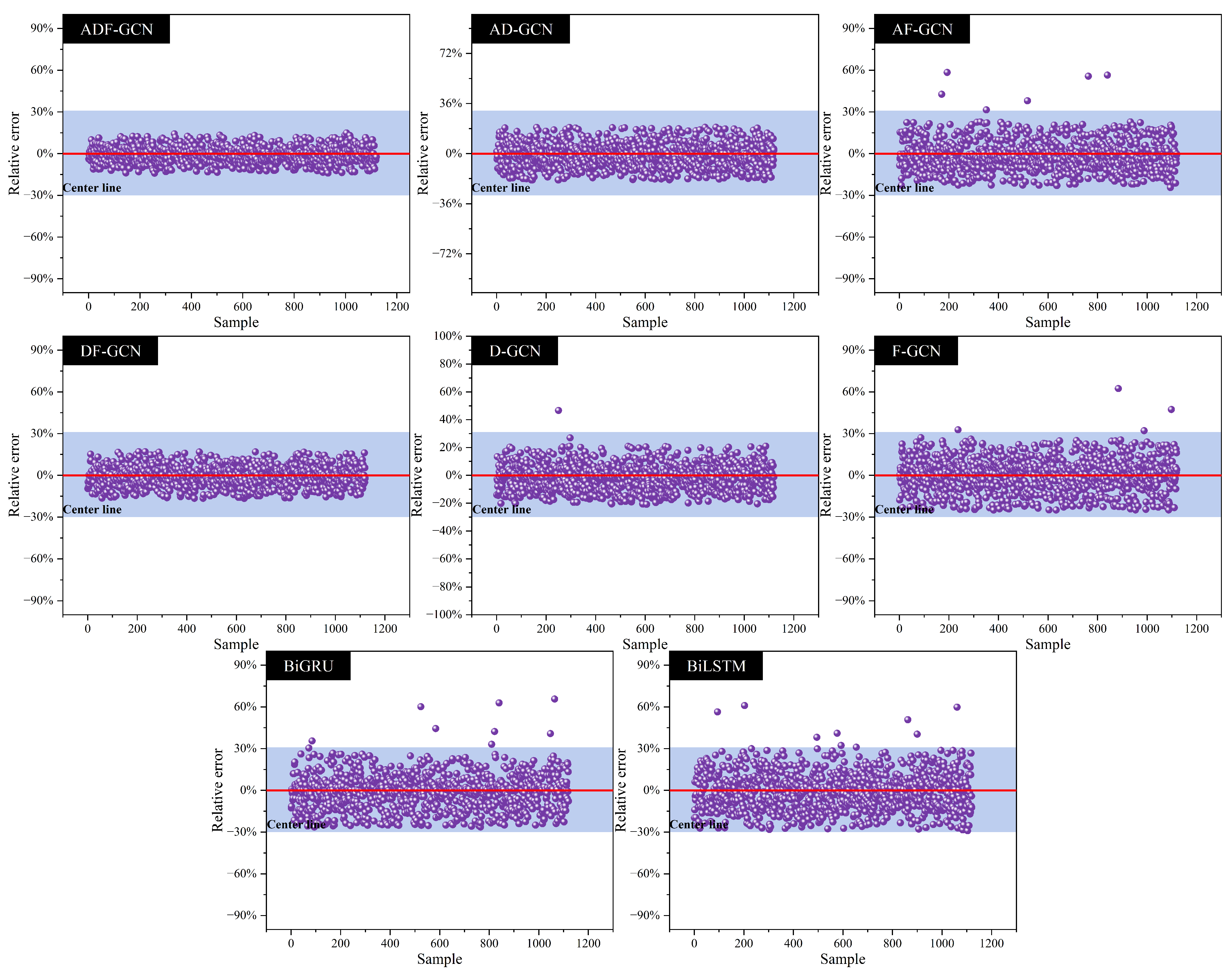
Figure 6 shows a scatter plot of the deep learning model’s relative error. A central line at 0% relative error was drawn. The proximity of the scatter points to the central line correlates positively with the model’s performance. Looking at the distribution of the scatter, the concentration is as follows: ADF-GCN (RMSE = 0.4873) > DF-GCN (RMSE = 0.6080) > AD-GCN (RMSE = 0.7169) > D-GCN (RMSE = 0.7858) > AF-GCN (RMSE = 0.8662) > F-GCN (RMSE = 0.9749) > BiGRU (RMSE = 1.0486) > BiLSTM (RMSE = 1.1552). Models based on GCNs were better at capturing complex geological structures for local information processing when dealing with sequential data. These models were adept at accommodating the intricate geological structures and data interdependencies present in the logging data. BiGRU (RMSE = 1.0486) and BiLSTM (RMSE = 1.1552) showed poorer performance; these two models are common variants of RNNs and are relatively strong in handling long-term dependencies in sequential information. These models might not have completely captured the intricate data patterns, due to insufficient local sequence feature extraction. Therefore, models based on GCNs had smaller relative errors and better performance, and were more capable of approaching the true values. The ADF-GCN model (RMSE = 0.4873), which considered both deep sequences and temporal-related graphs, and used an attention mechanism to generate an adaptive adjacency matrix, not only captured the correlations between deep sequences and features but also addressed the limitations of pre-built adjacency matrices, making its performance the best.
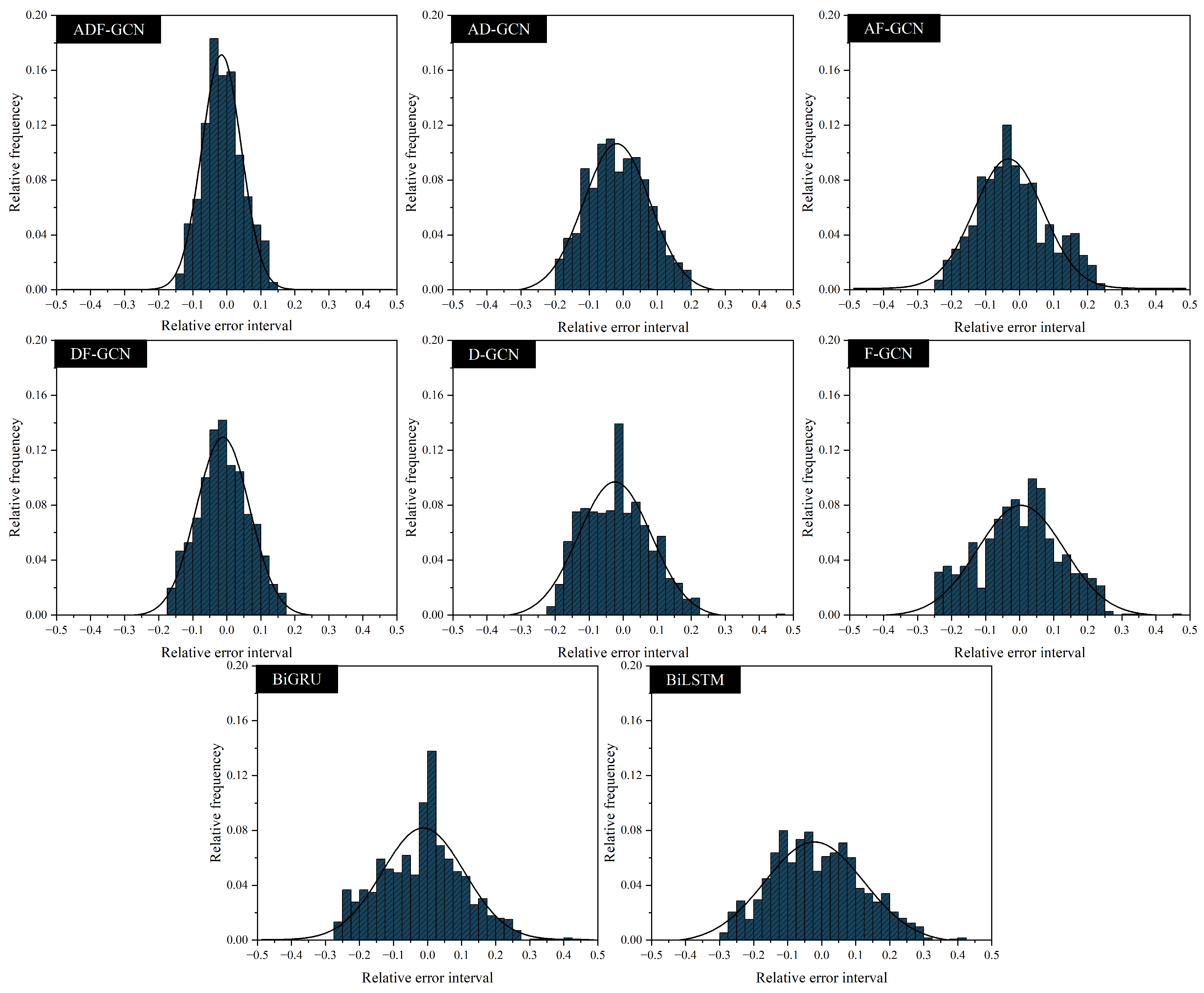
Figure 7 presents a scatter plot of the relative error intervals, alongside relative frequency histograms for the deep learning model. These charts were pivotal for assessing the model performance, providing insights into the model’s behavior across various error ranges, which aided in a more nuanced evaluation and refinement of the model. The chart’s x-axis denotes the relative error intervals, reflecting the gap between consecutive relative error values. The y-axis presents the relative frequency histogram, indicating the proportion of samples in each relative error interval against the total sample count. This dual-dimensional analysis enabled a thorough review of model performance on the chart. Notably, chart peaks suggest a concentration of samples in certain error intervals, hinting at the model’s stability and accuracy within those ranges. From the chart, it can be seen that the ADF-GCN (MAE = 0.4746) performed the best. This may be because it could better handle deep sequence data and capture complex geological structural information. Models based on GCNs generally have peaks closer to 0 than the RNN variants, including BiGRU (MAE = 0.7830) and BiLSTM (MAE = 0.9035). This suggests that even though RNNs variants are good at processing long-term dependent sequence information, undirected graphs are more suitable for capturing correlations between data, making them more applicable for identifying and combining logging data with high affinity or similarity.

5. Conclusions

In this study, we explored the feasibility and effectiveness of using an adaptive spectrogram convolution model which considers both depth sequence correlation graphs and feature correlation graphs for logging porosity prediction. Through ablation and comparison experiments, we found that the ADF-GCN performed well in this task, with significant performance advantages. The experimental results showed that the ADF-GCN exhibited better distribution characteristics in the relative error interval and relative frequency histogram. The chart’s peaks and positive curves demonstrate the model’s reliability and precision across various error ranges, visually affirming the ADF-GCN’s enhanced performance in predicting log porosity. We explored the rationale behind the model’s superior performance; the ADF-GCN model, by adaptively creating depth sequence correlation graphs and feature correlation graphs via an attention mechanism, transcends the constraints of static graph construction, substantially enhancing the prediction model’s precision and robustness. Additionally, by using a multi-head attention-based selection mechanism, we automatically detected and focuesed on key high-dimensional features resulting from the attention-aware graph convolution, efficiently eliminating redundant and overlapping information. Our study offers a robust approach to predicting logging porosity and introduces novel insights for the use of deep learning within geological and geoscience applications. The successful application of ADF-GCN in processing deep sequence data demonstrates its unique advantages and opens up new possibilities for further geoscientific tasks.
Despite the remarkable achievements of our research, there is still room for improvement. Future research could focus on optimizing the architecture and parameters of ADF-GCN to better adapt it to different geological structures and logging data types. Moreover, incorporating geological and geoscientific expertise could further refine the model’s capacity to comprehend and analyze geological characteristics. Collectively, our research presents a potent predictive tool for log porosity, a crucial contribution to the geosciences domain. We anticipate that our findings will offer valuable lessons and inspiration for subsequent studies, potentially advancing logging techniques and geoscientific research.

Author Contributions

L.H.: Writing—original draft (equal). X.W.: Writing—review and editing. Y.D.: Visualization. P.Z.: Writing—review and editing. P.H.: Writing—review and editing. X.L.: Writing—review and editing. F.J.: Methodology. C.Z.: Data curation. All authors have read and agreed to the published version of the manuscript.

Funding

This work was supported by National Key Research and Development Project of China (2021YFA1000103, 2021YFA1000102), National Natural Science Foundation of China (Grant Nos.62272479, 62372469, 62202498), Taishan Scholarship (tstp20240506), Shandong Provincial Natural Science Foundation (ZR2021QF023).

Institutional Review Board Statement

Not applicable.

Informed Consent Statement

Not applicable.

Data Availability Statement

The original contributions presented in the study are included in the article. Further inquiries can be directed to the corresponding author.

Conflicts of Interest

The authors declare no conflicts of interest.

Appendix A

Appendix A.1. Definition of Graph Determinacy Entropy

The structural determinacy of graphs can be quantified by the binary entropy of the adjacency matrix, defined as
H ( A ) = 1 N 2 i , j a i j log a i j + ( 1 a i j ) log ( 1 a i j ) ,
where binary entropy H ( A ) quantifies the structural determinacy of the graph through the adjacency matrix A = [ a i j ] , where a i j { 0 , 1 } indicates the presence of the edges between nodes i and j, N = | V | represents the total number of nodes, a i j log a i j captures the existence entropy of the edge (with 0 log 0 0 ), and ( 1 a i j ) log ( 1 a i j ) accounts for the uncertainty of the absence of the edge under identical zero convention.Crucially, lower entropy values indicate higher structural determinacy, as H ( A ) 0 corresponds to maximally certain connectivity patterns.
For the predefined deep sequence correlation graph (based on cosine similarity), setting the threshold θ = 0.7 yields an entropy value of H ( A d cos ) = 0.31 , indicating significant structural uncertainty. Further sensitivity analysis reveals that when θ increases from 0.6 to 0.8 , the entropy fluctuation Δ H = + 0.13 demonstrates the inherent threshold dependence of conventional methods. In contrast, the adaptively constructed deep sequence graph A d adp maintains a consistently low entropy ( H ( A d adp ) = 0.12 ) with negligible variation ( Δ H = 0.01 ) under threshold changes. This comparison clearly shows that the adaptive mechanism effectively mitigates threshold sensitivity through dynamic edge weight learning, resulting in substantially improved graph robustness.
For the predefined feature correlation graph (based on covariance signs), the entropy H ( A f cov ) = 0.28 , while slightly better than that of the predefined deep sequence graph, remains constrained by statistical assumptions. However, the adaptive feature graph achieves a significantly lower entropy of H ( A f adp ) = 0.15 . This highlights that feature correlation modeling requires overcoming both threshold dependency and statistical bias challenges, which the adaptive mechanism addresses through implicit encoding of non-Euclidean relationships via attention weights.

References

  1. Zhang, F.; Qiu, F.; Fang, Q.; Zhang, X.; Zhang, H.; Tang, F.; Fan, J. An accurately determining porosity method from pulsed-neutron element logging in unconventional reservoirs. In Proceedings of the SPWLA Annual Logging Symposium; OnePetro: Richardson, TX, USA, 2021; p. D041S037R001. [Google Scholar]
  2. Zhu, L.; Zhang, C.; Guo, C.; Jiao, Y.; Chen, L.; Zhou, X.; Zhang, C.; Zhang, Z. Calculating the total porosity of shale reservoirs by combining conventional logging and elemental logging to eliminate the effects of gas saturation. Petrophysics 2018, 59, 162–184. [Google Scholar] [CrossRef]
  3. An, P.; Yang, X.; Zhang, M. Porosity prediction and application with multiwell-logging curves based on deep neural network. In Proceedings of the SEG Technical Program Expanded Abstracts; Society of Exploration Geophysicists: Houston, TX, USA, 2018; pp. 819–823. [Google Scholar]
  4. Spinelli, R.; Magagnotti, N.; Nati, C. Benchmarking the impact of traditional small-scale logging systems used in Mediterranean forestry. Forest Ecol. Manag. 2010, 260, 1997–2001. [Google Scholar] [CrossRef]
  5. Zhou, K.; Hu, Y.; Pan, H.; Kong, L.; Liu, J.; Huang, Z.; Chen, T. Fast prediction of reservoir permeability based on embedded feature selection and LightGBM using direct logging data. Meas. Sci. Technol. 2020, 31, 045101. [Google Scholar] [CrossRef]
  6. Merembayev, T.; Yunussov, R.; Yedilkhan, A. Machine learning algorithms for classification geology data from well logging. In Proceedings of the 14th International Conference on Electronics Computer and Computation (ICECCO), Kaskelen, Kazakhstan, 29 November–1 December 2018; IEEE: Piscataway, NJ, USA, 2018; pp. 206–212. [Google Scholar]
  7. Alqahtani, N.; Armstrong, R.T.; Mostaghimi, P. Deep learning convolutional neural networks to predict porous media properties. In Proceedings of the SPE Asia Pacific Oil and Gas Conference and Exhibition, Brisbane, Australia, 23–25 October 2018; SPE: Calgary, AB, Canada, 2018; p. D012S032R010. [Google Scholar]
  8. Santos, J.E.; Xu, D.; Jo, H.; Landry, C.J.; Prodanović, M.; Pyrcz, M.J. PoreFlow-Net: A 3D convolutional neural network to predict fluid flow through porous media. Adv. Water Resour. 2020, 138, 103539. [Google Scholar] [CrossRef]
  9. Zhang, F.; He, X.; Teng, Q.; Wu, X.; Dong, X. 3D-PMRNN: Reconstructing three-dimensional porous media from the two-dimensional image with recurrent neural network. J. Pet. Sci. Eng. 2022, 208, 109652. [Google Scholar] [CrossRef]
  10. Wang, J.; Cao, J.; Zhou, X. Reservoir porosity prediction based on deep bidirectional recurrent neural network. Prog. Geophys. 2022, 37, 267–274. [Google Scholar]
  11. Song, X.; Liu, Y.; Xue, L.; Wang, J.; Zhang, J.; Wang, J.; Jiang, L.; Cheng, Z. Time-series well performance prediction based on Long Short-Term Memory (LSTM) neural network model. J. Pet. Sci. Eng. 2020, 186, 106682. [Google Scholar] [CrossRef]
  12. Shi, S.Z.; Shi, G.F.; Pei, J.B.; Zhao, K.; He, Y.Z. Porosity prediction in tight sandstone reservoirs based on a one–dimensional convolutional neural network–gated recurrent unit model. Appl. Geophys. 2023, 1–13. [Google Scholar] [CrossRef]
  13. Yu, Z.; Sun, Y.; Zhang, J.; Zhang, Y.; Liu, Z. Gated recurrent unit neural network (GRU) based on quantile regression (QR) predicts reservoir parameters through well logging data. Front. Earth Sci. 2023, 11, 1087385. [Google Scholar] [CrossRef]
  14. Zeng, L.; Ren, W.; Shan, L. Attention-based bidirectional gated recurrent unit neural networks for well logs prediction and lithology identification. Neurocomputing 2020, 414, 153–171. [Google Scholar] [CrossRef]
  15. Yang, L.; Wang, S.; Chen, X.; Chen, W.; Saad, O.M.; Zhou, X.; Pham, N.; Geng, Z.; Fomel, S.; Chen, Y. High-fidelity permeability and porosity prediction using deep learning with the self-attention mechanism. IEEE Trans. Neural Netw. Learn. Syst. 2022, 34, 3429–3443. [Google Scholar] [CrossRef] [PubMed]
  16. Chen, W.; Yang, L.; Zha, B.; Zhang, M.; Chen, Y. Deep learning reservoir porosity prediction based on multilayer long short-term memory network. Geophysics 2020, 85, WA213–WA225. [Google Scholar] [CrossRef]
  17. Shan, L.; Liu, Y.; Tang, M.; Yang, M.; Bai, X. CNN-BiLSTM hybrid neural networks with attention mechanism for well log prediction. J. Pet. Sci. Eng. 2021, 205, 108838. [Google Scholar] [CrossRef]
  18. Ersavas, T.; Smith, M.A.; Mattick, J.S. Novel applications of Convolutional Neural Networks in the age of Transformers. Sci. Rep. 2024, 14, 10000. [Google Scholar] [CrossRef]
  19. Li, Z.; Yu, J.; Zhang, G.; Xu, L. Dynamic spatio-temporal graph network with adaptive propagation mechanism for multivariate time series forecasting. Expert Syst. Appl. 2023, 216, 119374. [Google Scholar] [CrossRef]
  20. Yang, J.; Xie, F.; Yang, J.; Shi, J.; Zhao, J.; Zhang, R. Spatial-temporal correlated graph neural networks based on neighborhood feature selection for traffic data prediction. Appl. Intell. 2023, 53, 4717–4732. [Google Scholar] [CrossRef]
  21. Guo, S.; Lin, Y.; Feng, N.; Song, C.; Wan, H. Attention based spatial-temporal graph convolutional networks for traffic flow forecasting. In Proceedings of the AAAI Conference on Artificial Intelligence, Honolulu, HI, USA, 27 January–1 February 2019; Volume 33, pp. 922–929. [Google Scholar]
  22. Wang, X.; Zhao, J.; Zhu, L.; Zhou, X.; Li, Z.; Feng, J.; Deng, C.; Zhang, Y. Adaptive multi-receptive field spatial-temporal graph convolutional network for traffic forecasting. In Proceedings of the 2021 IEEE Global Communications Conference (GLOBECOM), Madrid, Spain, 7–11 December 2021; IEEE: Piscataway, NJ, USA, 2021; pp. 1–7. [Google Scholar]
  23. Wang, Y.; Ren, Q.; Li, J. Spatial–temporal multi-feature fusion network for long short-term traffic prediction. Expert Syst. Appl. 2023, 224, 119959. [Google Scholar] [CrossRef]
  24. Cai, K.; Shen, Z.; Luo, X.; Li, Y. Temporal attention aware dual-graph convolution network for air traffic flow prediction. J. Air Transp. Manag. 2023, 106, 102301. [Google Scholar] [CrossRef]
  25. Tao, B.; Liu, X.; Zhou, H.; Liu, J.; Lyu, F.; Lin, Y. Porosity prediction based on a structural modeling deep learning method. Geophysics 2024, 89, 1–73. [Google Scholar] [CrossRef]
  26. Yuan, C.; Wu, Y.; Li, Z.; Zhou, H.; Chen, S.; Kang, Y. Lithology identification by adaptive feature aggregation under scarce labels. J. Pet. Sci. Eng. 2022, 215, 110540. [Google Scholar] [CrossRef]
  27. Feng, S.; Li, X.; Zeng, F.; Hu, Z.; Sun, Y.; Wang, Z.; Duan, H. Spatiotemporal deep learning model with graph convolutional network for well logs prediction. IEEE Geosci. Remote Sens. Lett. 2023, 20, 7505205. [Google Scholar] [CrossRef]
  28. Li, T.; Zhao, Z.; Sun, C.; Yan, R.; Chen, X. Multireceptive field graph convolutional networks for machine fault diagnosis. IEEE Trans. Ind. Electron. 2020, 68, 12739–12749. [Google Scholar] [CrossRef]
  29. Wei, Y.; Wu, D. Prediction of state of health and remaining useful life of lithium-ion battery using graph convolutional network with dual attention mechanisms. Reliab. Eng. Syst. Saf. 2023, 230, 108947. [Google Scholar] [CrossRef]
  30. Lin, Z.; Feng, M.; Santos, C.N.d.; Yu, M.; Xiang, B.; Zhou, B.; Bengio, Y. A structured self-attentive sentence embedding. arXiv 2017, arXiv:1703.03130. [Google Scholar]
  31. Hammond, D.K.; Vandergheynst, P.; Gribonval, R. Wavelets on graphs via spectral graph theory. Appl. Comput. Harmon. Anal. 2011, 30, 129–150. [Google Scholar] [CrossRef]
  32. Ellis, D.V.; Singer, J.M. Lithology and Porosity Estimation. In Well Logging for Earth Scientists; Springer: Berlin/Heidelberg, Germany, 2007; pp. 629–652. [Google Scholar]
  33. Helle, H.B.; Bhatt, A.; Ursin, B. Porosity and permeability prediction from wireline logs using artificial neural networks: A North Sea case study. Geophys. Prospect. 2001, 49, 431–444. [Google Scholar] [CrossRef]
  34. Soete, J.; Kleipool, L.M.; Claes, H.; Claes, S.; Hamaekers, H.; Kele, S.; Özkul, M.; Foubert, A.; Reijmer, J.J.; Swennen, R. Acoustic properties in travertines and their relation to porosity and pore types. Mar. Pet. Geol. 2015, 59, 320–335. [Google Scholar] [CrossRef]
  35. de Oliveira, J.M., Jr.; Andreo Filho, N.; Chaud, M.V.; Angiolucci, T.; Aranha, N.; Martins, A.C.G. Porosity measurement of solid pharmaceutical dosage forms by gamma-ray transmission. Appl. Radiat. Isot. 2010, 68, 2223–2228. [Google Scholar] [CrossRef]
  36. Wu, W.; Tong, M.; Xiao, L.; Wang, J. Porosity sensitivity study of the compensated neutron logging tool. J. Pet. Sci. Eng. 2013, 108, 10–13. [Google Scholar] [CrossRef]
  37. Xu, B.S.; Li, N.; Xiao, L.Z.; Wu, H.L.; Wang, B.; Wang, K.W. Serial structure multi-task learning method for predicting reservoir parameters. Appl. Geophys. 2022, 19, 513–527. [Google Scholar] [CrossRef]
  38. Sun, Y.; Zhang, J.; Yu, Z.; Zhang, Y.; Liu, Z. Bidirectional long short-term neural network based on the attention mechanism of the residual neural network (ResNet–BiLSTM–attention) predicts porosity through well logging parameters. ACS Omega 2023, 8, 24083–24092. [Google Scholar] [CrossRef] [PubMed]
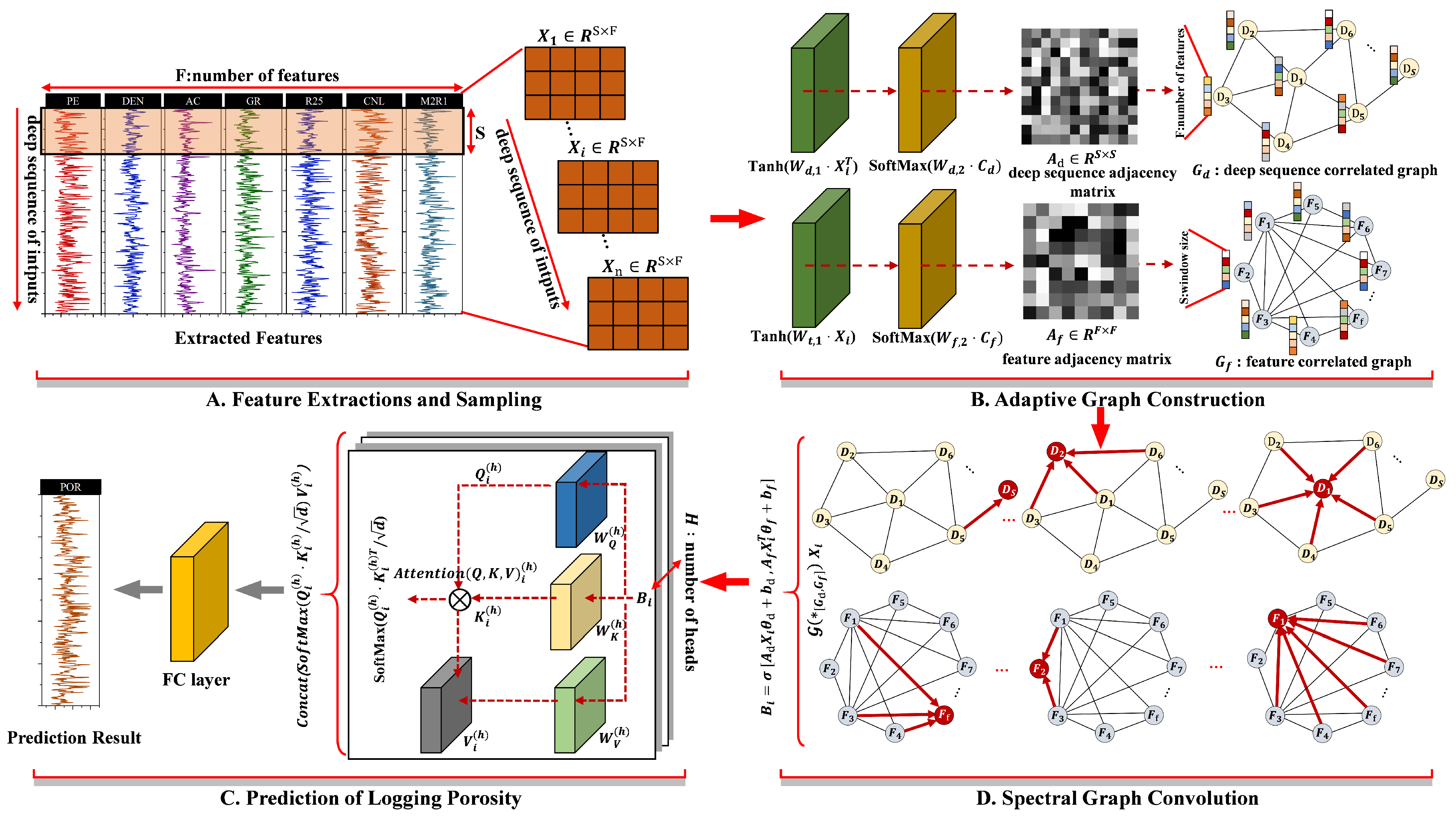
Figure 1. The computational framework for the adaptive graph convolution operation with sequence and feature correlation graphs includes (A) feature extraction and sampling, (B) adaptive construction of graphs, (C) spectral graph convolution operations for both graphs, and (D) porosity prediction based on multi-head attention.
Applsci 15 04609 g001
Figure 2. Histogram of the distribution of logging parameters and porosity data.
Applsci 15 04609 g002
Figure 3. Violin diagrams of logging parameters and porosity data.
Applsci 15 04609 g003
Figure 4. Scatter plot of the true and predicted values of the deep learning models on the training set.
Applsci 15 04609 g004
Figure 5. Scatter plot of the true and predicted values of the deep learning models on the testing set.
Applsci 15 04609 g005
Figure 6. Scatter plot of relative error of deep learning models.
Applsci 15 04609 g006
Figure 7. Histograms of the relative error interval and relative frequency of the deep learning models.
Applsci 15 04609 g007
Table 1. Well-logging parameters and porosity statistics table.
Logging ParametersMaxMinMeanMedianStandard DeviationSkewness
PE 6.10 3.31 3.39 4.17 0.14 1.97
DEN 2.62 2.53 2.57 2.58 0.02 0.16
AC 62.56 55.06 57.30 57.26 1.18 1.27
GR 67.98 39.24 46.94 47.69 5.36 1.87
R25 148.38 111.04 125.88 126.56 5.18 0.78
CNL 11.81 5.08 7.73 7.80 3.30 0.46
M2R1 787.56 143.71 349.97 67.25 67.25 0.98
POR 12.97 2.32 6.30 6.56 1.71 0.7
Table 2. Abbreviations and descriptions of ablation and comparison experiments.
ExperimentsAbbreviationsParticulars
Ablation ExperimentsADF-GCNAdaptive GCN for deep sequence and feature correlation graph (ours)
AD-GCNAdaptive GCN for deep sequence correlation graph
AF-GCNAdaptive GCN for feature correlation graph
DF-GCNGCN for deep sequence and feature correlation graph
D-GCNGCN for deep sequence correlation graph
F-GCNGCN for feature correlation graph
Comparison ExperimentsBiGRU [37]Bidirectional Gated Recurrent Unit
BiLSTM [38]Bidirectional Long Short-Term Memory
Table 3. Deep learning model parameters.
ModelsParametersValues
Ablation Model Ensemble *Graph convolution layer4
The number of heads2
The window size12
Activation functionReLU
Learning rate 1 × 10 4
OptimizerAdam
Dropout0.3
Maximum iterations1000
Batch size32
BiGRUThe number of GRU units in each layer128
Activation functionReLU
Learning rate 1 × 10 4
OptimizerAdam
Dropout0.3
Maximum iterations1000
Batch size32
BiLSTMThe number of LSTM units in each layer128
Activation functionReLU
Learning rate 1 × 10 4
OptimizerAdam
Dropout0.3
Maximum iterations1000
Batch size32
* Ablation model ensemble includes ADF-GCN, AD-GCN, AF-GCN, DF-GCN, D-GCN and F-GCN.
Table 4. Values of the four evaluation indicators of the deep learning models (The bold and underlined values indicate the best results).
ModelRMSER2MAEMAPE
Dataset Train TestTrainTestTrainTestTrainTest
ADF-GCN0.4870.5060.9510.9480.3470.0.3786.389%6.733%
AD-GCN0.7200.7460.8940.8870.5750.5869.930%10.162%
AF-GCN0.8660.9160.8450.8300.6780.70412.080%12.656%
DF-GCN0.6080.6380.9240.9170.4750.4878.365%8.670%
D-GCN0.7860.8510.8720.8540.6080.64210.743%11.596%
F-GCN0.9750.9980.8080.7940.7280.76411.623%12.124%
BiGRU1.0491.0610.7770.7670.7830.79413.567%13.619%
BiLSTM1.1551.1560.7300.7230.9040.91315.293%15.327%
Disclaimer/Publisher’s Note: The statements, opinions and data contained in all publications are solely those of the individual author(s) and contributor(s) and not of MDPI and/or the editor(s). MDPI and/or the editor(s) disclaim responsibility for any injury to people or property resulting from any ideas, methods, instructions or products referred to in the content.