Abstract
The electric solar wind sail (E-sail) is a propellantless propulsion system concept based on the use of a system of very long and thin conducting tethers, which create an artificial electric field that is able to deflect the solar-wind-charged particles in order to generate a net propulsive acceleration outside the planetary magnetospheres. The radial rig of conducting tethers is deployed and stretched by rotating the spacecraft about an axis perpendicular to the nominal plane of the sail. This rapid rotation complicates the thrust vectoring of the E-sail-based spacecraft, which is achieved by changing the orientation of the sail nominal plane with respect to an orbital reference frame. For this reason, some interesting steering techniques have recently been proposed which are based, for example, on maintaining the inertial direction of the spacecraft spin axis or on limiting the excursion of the so-called pitch angle, which is defined as the angle formed by the unit vector perpendicular to the sail nominal plane with the (radial) direction of propagation of the solar wind. In this paper, a different control strategy based on maintaining the pitch angle value constant during a typical interplanetary flight is investigated. In this highly constrained configuration, the spacecraft spin axis can rotate freely around the radial direction, performing a sort of conical motion around the Sun-vehicle line. Considering an interplanetary Earth–Venus or Earth–Mars mission scenario, the flight performance is here compared with a typical unconstrained optimal transfer, aiming to quantify the flight time variation due to the pitch angle value constraint. In this regard, simulation results indicate that the proposed control law provides a rather limited (percentage) performance variation in the case where the reference propulsive acceleration of the E-sail-based spacecraft is compatible with a medium- or low-performance propellantless propulsion system.
1. Introduction
A spacecraft propellantless propulsion system allows the design of space trajectories that are difficult to achieve using conventional thrusters, due to the well-known limitation related to the finite mass of propellant that can be carried on board the spacecraft. In the still very narrow field of propellantless propulsion systems for space vehicles, the electric solar wind sail (E-sail) [1,2] and concepts derived from it, such as the interesting plasma brake [3,4,5], represent a fascinating and effective alternative to the more well-known and technologically mature photonic solar sails [6,7,8]. Unlike the latter, which essentially uses a large, lightweight mirror-like surface to reflect incoming photons, an E-sail uses a large rig of long, thin, conducting tethers to create an artificial electric field that deflects the charged particles carried by the solar wind, in order to provide a (propellantless) net propulsive acceleration to a spacecraft operating in a heliocentric mission scenario, i.e., outside the typical planetary magnetospheres [9,10].
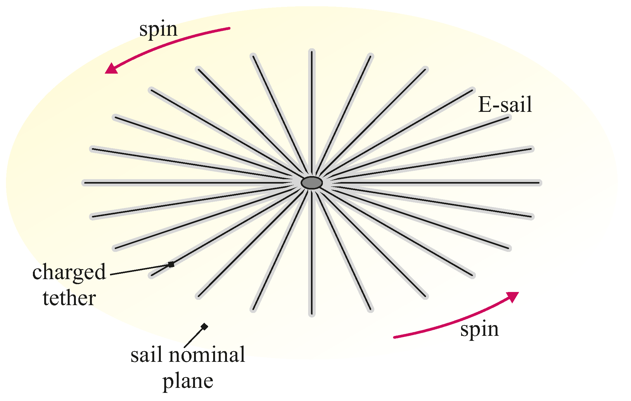
The radial rig of conducting tethers is deployed and stretched by rotating the vehicle about an axis perpendicular to the nominal plane of the sail [11,12,13] with a suitable angular velocity, which is consistent with the mechanical characteristics of the metallic wires that form the generic multiline tether [14,15]. The conceptual scheme of a rotating E-sail is reported in Figure 1. The space vehicle’s rotation imparts an inherent gyroscopic stiffness to the system, which complicates the thrust vectoring of the E-sail-based spacecraft, which is achieved by changing the orientation of the sail nominal plane with respect to an orbital reference frame [16,17,18]. For this reason, over the years, several control and guidance strategies have been proposed that are able to modify both the spin rate and the attitude of the E-sail-propelled spacecraft, in order to allow the achievement of a given heliocentric orbital transfer with acceptable performances in terms of total flight time [19]. In this regard, the interested reader is referred to the fundamental works of Toivanen and Janhunen [20,21,22,23,24], who, for the first time, addressed and discussed the considerable problem of the in-flight attitude variation of a large space structure as an E-sail of medium propulsive performances.
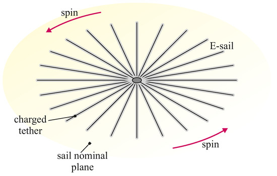
Figure 1.
Diagram of a spinning E-sail with the nominal plane highlighted in yellow.
In the context of a simplified E-sail guidance control during a typical interplanetary flight, some interesting steering techniques have recently been investigated which are based, for example, on maintaining the inertial direction of the spacecraft spin axis [25,26] or on limiting the excursion of the so-called sail pitch angle [27]. The latter, borrowing the nomenclature introduced in the design of the photonic solar sail control law [28,29], is defined as the angle formed by the unit vector perpendicular to the sail nominal plane (in direction opposite to the Sun) with the direction of propagation of the solar wind, which is usually assumed as coincident with the (radial) Sun–spacecraft line. Indeed, assuming a classical axially symmetric E-sail, the possibility of maintaining a constant value of the pitch angle of the vehicle during flight, as described in the interesting approach illustrated in ref. [30], allows the mission designer to theoretically conceive a simplified steering law in which the pitch angle can be freely selected in a finite set of possible values. The latter is, in fact, substantially the approach used by Jin et al. [31,32,33] in their elegant works on the study of the heliocentric motion of an E-sail-propelled spacecraft with a fixed direction of the thrust vector (in the orbital reference frame) using an approximate semi-analytic approach, which is based on classical linear perturbation theory. In fact, according to the well-known analytical thrust model proposed by Huo et al. in 2018 [34], the direction of the thrust vector induced by the E-sail is strictly connected to the direction of the unit vector normal to the sail nominal plane. In particular, a constant value of the pitch angle corresponds to a constant (and usually very small) value of the sail cone angle, defined as the angle formed by the thrust vector with the propagation direction of the solar wind. Note that the term pitch angle does not coincide with the one usually used to indicate one of the three rotations between the body axes and the orbital frame’s axes, i.e., one of the three Euler angles.
In this paper, a different control strategy is examined based on keeping the sail pitch angle value constant during the whole interplanetary flight, and using an optimization approach to derive the actual, optimal form of the spacecraft transfer trajectory. In this context, the nonlinear equations of motion of the vehicle in the heliocentric frame are considered and numerically integrated, through an automated routine based on a classical predictor-corrector method [35,36]. In this specific, pitch angle-constrained, E-sail configuration, the spin axis of the axially symmetric spacecraft can rotate freely around the direction of solar wind propagation, performing a sort of conical motion, allowing the sail nominal plane (and then the propulsive acceleration vector) to vary its azimuthal orientation in an orbital reference frame in order to obtain a desired thrust vectoring. In fact, in an orbital reference frame, the spacecraft spin axis, which is perpendicular to the nominal plane of the sail, describes a circular cone having an aperture equal to twice the (fixed) sail pitch angle, and whose axis coincides with the Sun–spacecraft radial line. This situation is schematically illustrated in the diagram shown in Figure 2, where the circular cone on whose external surface the unit vector normal to the sail nominal plane is constrained to lie contains, within itself, the thrust vector of the E-sail.
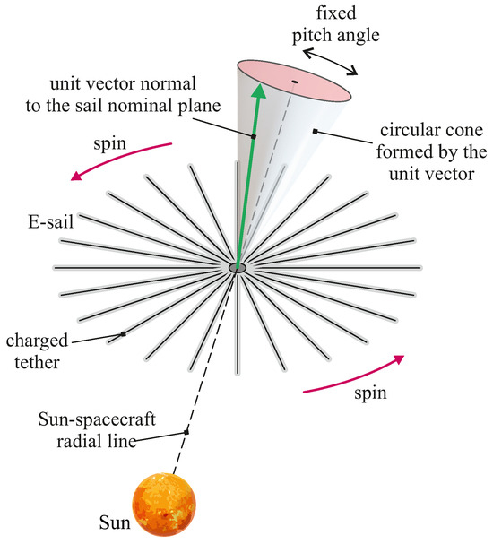
Figure 2.
Conceptual sketch of an E-sail-propelled spacecraft, in a heliocentric scenario, with a constant pitch angle. The unit vector normal to the sail nominal plane (in the direction opposite to the Sun) is constrained to lie on the surface of a circular cone whose aperture is equal to twice the fixed sail pitch angle.
This interesting guidance law reduces to one the number of control angles that can be freely selected during interplanetary flight, and therefore significantly simplifies, at least from a conceptual point of view, the problem of the sail attitude variation during a heliocentric orbital transfer. The mathematical description of the constrained thrust model of a spinning E-sail is illustrated in Section 2. The fixed sail pitch angle-based control strategy, which has been shown in the past to be really effective in a photonic solar sail-propelled heliocentric mission scenario [37], is analyzed here by considering a classical three-dimensional interplanetary orbit-to-orbit transfer between the Earth and two of the three remaining terrestrial planets, namely Venus and Mars. The two interplanetary mission scenarios, together with some notes on the design of the optimal transfer trajectory, allowing the potential reader to refer to recent literature, are illustrated in Section 3. Accordingly, the work extends to an E-sail-based mission scenario the literature results regarding this potential simplified guidance law. The numerical results, in terms of the minimum flight time as a function of the propulsive (reference) characteristics of the E-sail, are then compared with a typical unconstrained optimal transfer, with the aim of quantifying the performance degradation due to the assumed constraint of the pitch angle value during the whole transfer.
In this regard, as discussed in Section 4, the numerical results obtained by simulations indicate that this simplified (constrained) steering law provides a rather limited performance variation in the case where the reference propulsive acceleration of the E-sail is compatible with a medium performance propellantless propulsion system. However, a careful analysis of the generic interplanetary mission scenario indicates that the performance degradation obtained using a constrained guidance law is strictly related to the specific value of the pitch angle selected during the transfer. In this regard, Section 4 contains a parametric study of the problem where the total flight time is obtained, for a given mission scenario, as a function of the selected sail pitch angle. Such a parametric study allows the best value of the sail pitch angle to be obtained in order to minimize the performance degradation in an assigned mission scenario and for a given E-sail reference propulsive acceleration level. Finally, Section 5 concludes the paper.
2. Sail Pitch Angle Constrained Thrust Model of the E-Sail
Bearing in mind that the E-sail is a propellantless propulsion system and, therefore, the mass of the spacecraft hosting this thruster is a constant of motion, it is more convenient to use the propulsive acceleration vector instead of the classical thrust vector during the preliminary phase of the mission design. In this context, the expression of can be obtained by resorting to the elegant approach proposed by Huo et al. [34], which allows the expression of the acceleration vector induced by the E-sail as a function of the Sun–spacecraft distance r; the radial unit vector indicating the direction of the solar wind flow; the unit vector normal to the shadowed side of the sail nominal plane; the maximum magnitude of the propulsive acceleration (also referred to as characteristic acceleration) at a reference solar distance ; the thruster switching parameter modeling the on/off behavior of the E-sail due to the possibility of zeroing the artificial electric field by changing the tethers’ voltage. In particular, according to ref. [34], the compact form of the propulsive acceleration vector is given by
where it can be observed that, when (i.e., E-sail turned on), (i.e., the spacecraft solar distance is one astronomical unit), and (i.e., the normal direction coincides with the radial one), one has , as expected. In that case, the sail nominal plane is perpendicular to the direction of the solar wind flow, and the E-sail has a Sun-facing attitude. According to their definition, the sail pitch angle can be considered as the angle between the two unit vectors and , so that we simply have the following expression
which allows the propulsive acceleration magnitude to be written as [34]
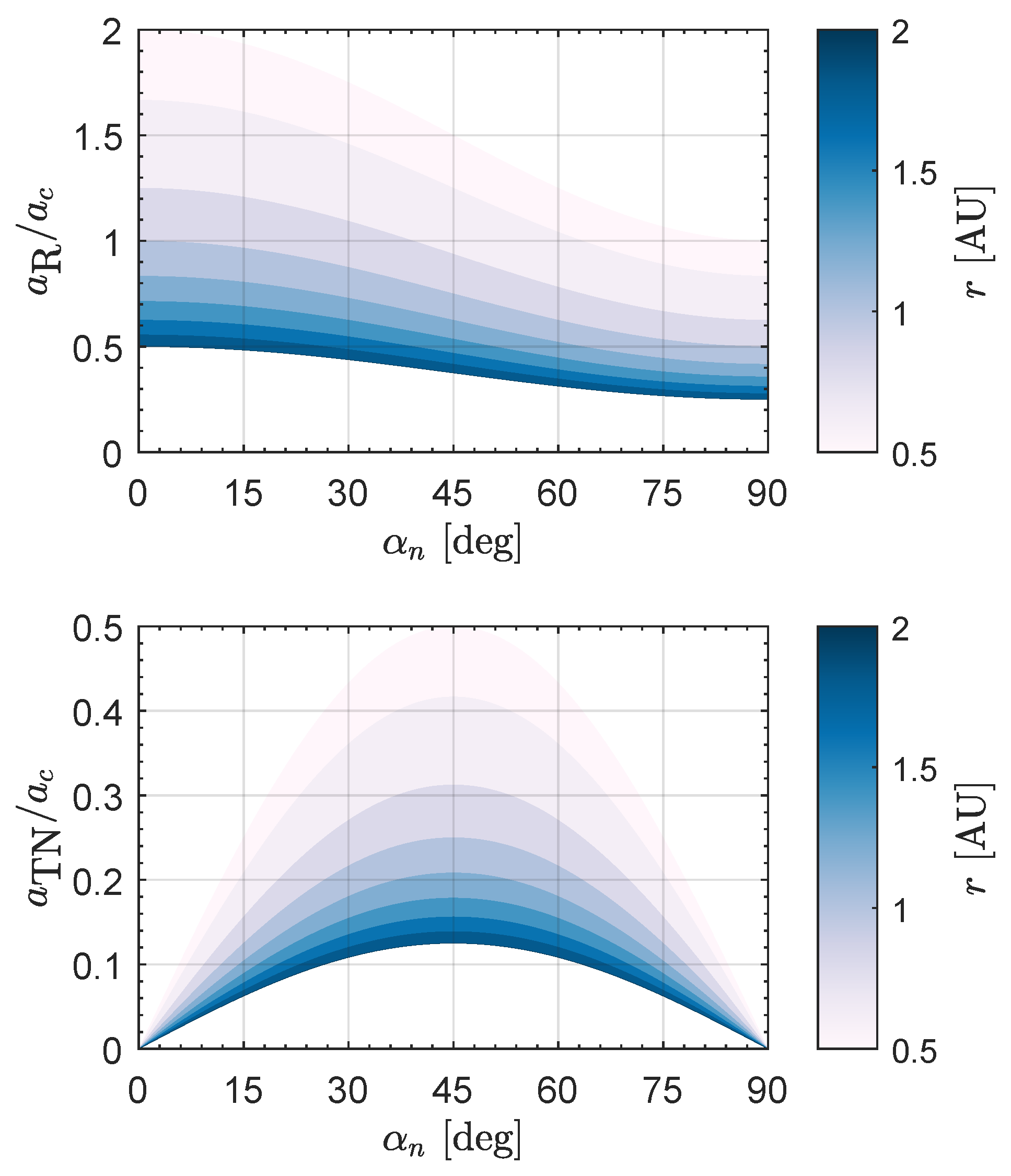
The variation of the dimensionless ratio with r and , obtained through the previous equation, has been plotted in Figure 3, where it can be observed that, at a distance from the star consistent with the average Sun–Venus (or Sun–Mars) distance, the maximum value of the magnitude of the propulsive acceleration vector is about greater (or less) than .
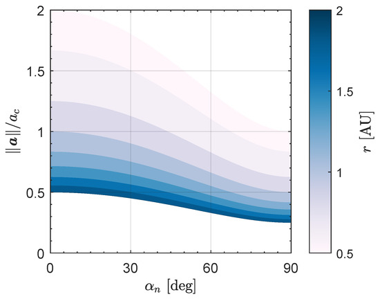
Figure 3.
Variation of the dimensionless ratio with and for an E-sail with , i.e., for a propulsion system turned on.
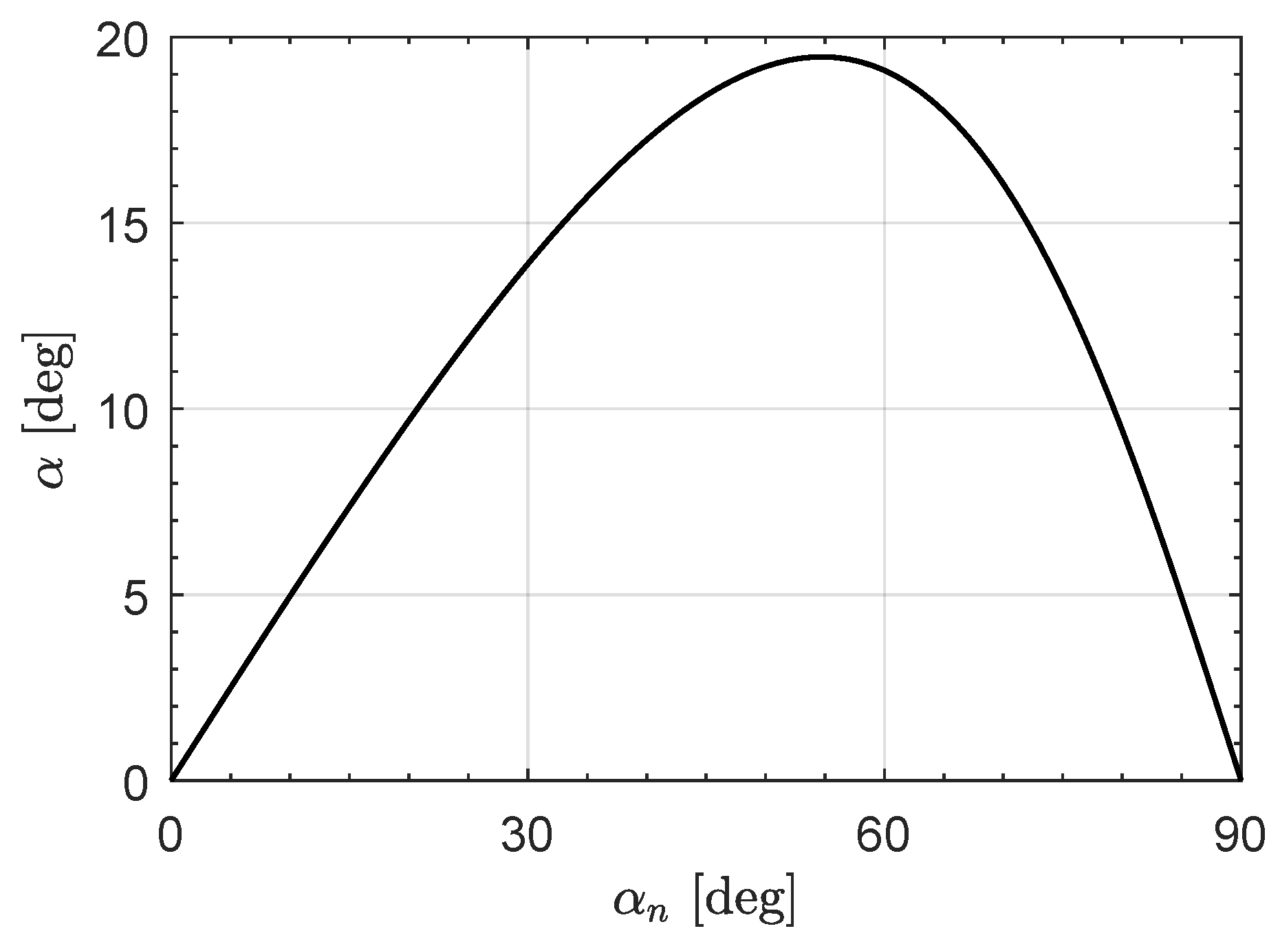
Finally, the sail cone angle , that is, the angle between the Sun–spacecraft line and the direction of the propulsive acceleration vector can be obtained from Equation (1) as
whose graph, reported in Figure 4, indicates that the maximum value of the cone angle is slightly less than . This value is reached when the pitch angle of the E-sail is approximately equal to . Note, in passing, that this last value of corrects a typing error in the last part of Equation (21) in ref. [34].

Figure 4.
Variation of the sail cone angle with the sail pitch angle , when the E-sail is turned on.
In order to highlight the dependence of the propulsive acceleration from the sail pitch angle, the vector is projected in a classical radial-transverse-normal reference frame , whose origin coincides with the spacecraft center of mass. In particular, the unit vectors are related to the inertial position vector and the velocity vector of the E-sail-based spacecraft through the well-known expressions
Introducing the clock angle defined as the angle between the direction of the unit vector and the projection of the sail normal unit vector into the plane , one has
so that Equation (1) can be rewritten in a compact form as
where and are two functions of r and defined as
Note that (or ) coincides with the radial (or the transversal) component of the local propulsive acceleration vector when the E-sail is turned on. The two components are shown, in a dimensionless form, in Figure 5, in which one can observe that the maximum value of the transversal component is reached when .

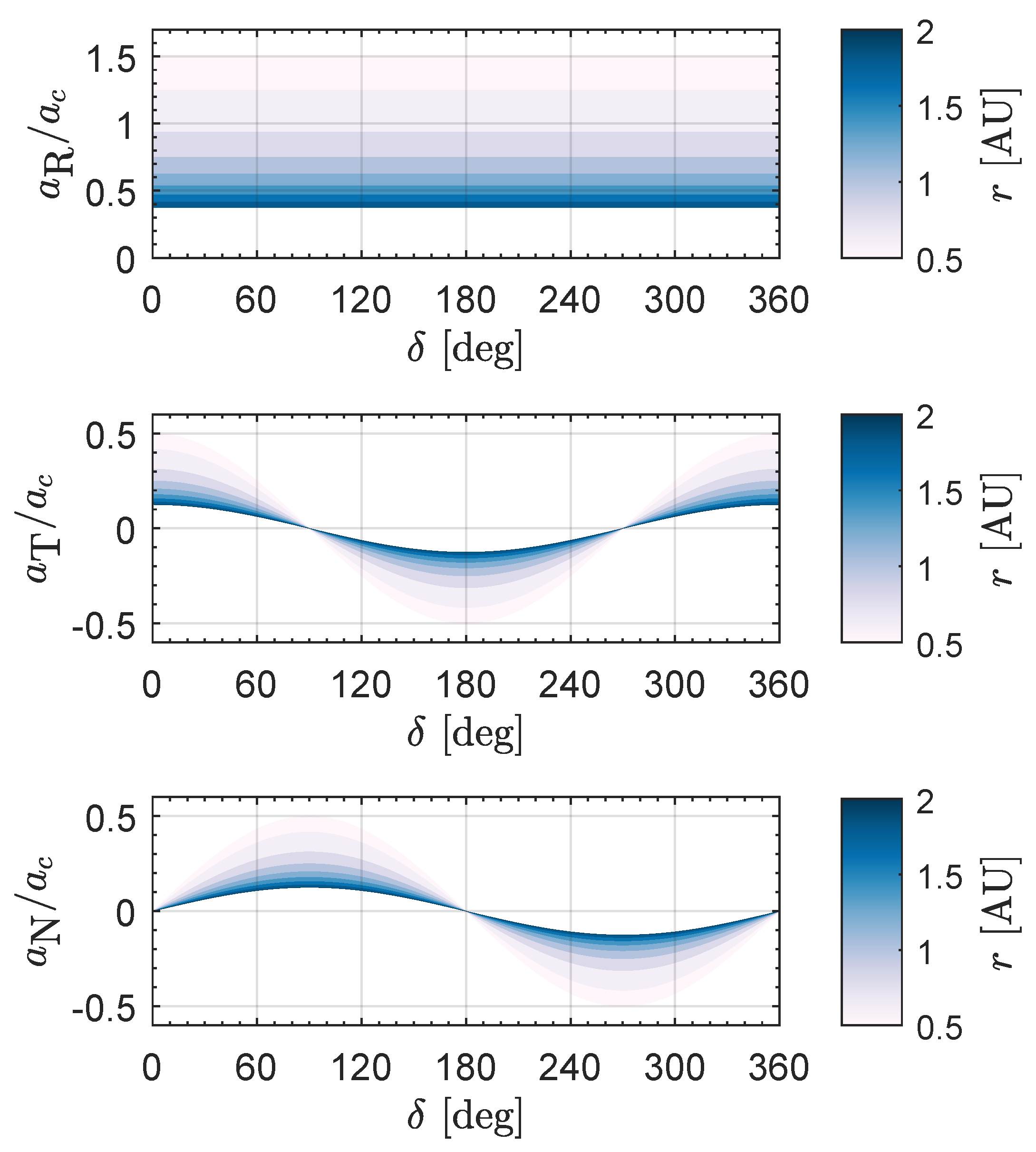
Figure 5.
Variation of the dimensionless radial component and the transversal component of the propulsive acceleration vector with and .
Consequently, at a generic solar distance r and for a given value of the sail pitch angle , which is maintained throughout all the interplanetary flight, the value of the two terms is given by Equations (8) and (9), so that the control variables are the two dimensionless terms and which appear in the right side of Equation (7). For example, in the important case of , that is, in the case where the transversal component of the propulsive acceleration vector is maximized, Figure 6 shows the variation of the three components of in the radial-transverse-normal reference frame as a function of the clock angle and the solar distance r, when the E-sail is turned on; see also Equation (7). However, it should be noted that, for a given mission scenario, the (fixed) value of the sail pitch angle must be carefully selected, in order to avoid excessively long flight times or even to try to obtain a physically unfeasible orbital transfer. In this regard, in fact, taking into account Equation (1) or the graphs reported in Figure 5, it is observed that in the two particular cases in which , the direction of the thrust vector is purely radial, that is, . In these cases, the presence of a radial outward propulsive acceleration entails the conservation of the semilatus rectum of the spacecraft osculating orbit, that is, of the magnitude of the specific angular momentum vector [38,39,40]. Consequently, it is not physically possible to perform a transfer between two heliocentric (Keplerian) orbits that do not share the same value of the semilatus rectum. On the other hand, the case where has a very small value (or a value near to ) corresponds to a scenario where the transversal component of the propulsive acceleration is very small, and this leads to a large flight time in heliocentric scenarios where the semilatus rectum of the target orbit is very different from that of the parking orbit, as in the typical case of an interplanetary transfer.

Figure 6.
Dimensionless components of acceleration vector in as a function of and , when and . In the graph, and .
In all other cases, the time variation of the two control terms can be obtained by optimizing an assigned performance index—as, for example, the total flight time—in a given mission scenario, in order to ensure the transfer of the E-sail propelled spacecraft between two given heliocentric orbits. This aspect is briefly illustrated in the next section.
3. Description of the Mission Scenarios and Notes on the Trajectory Design
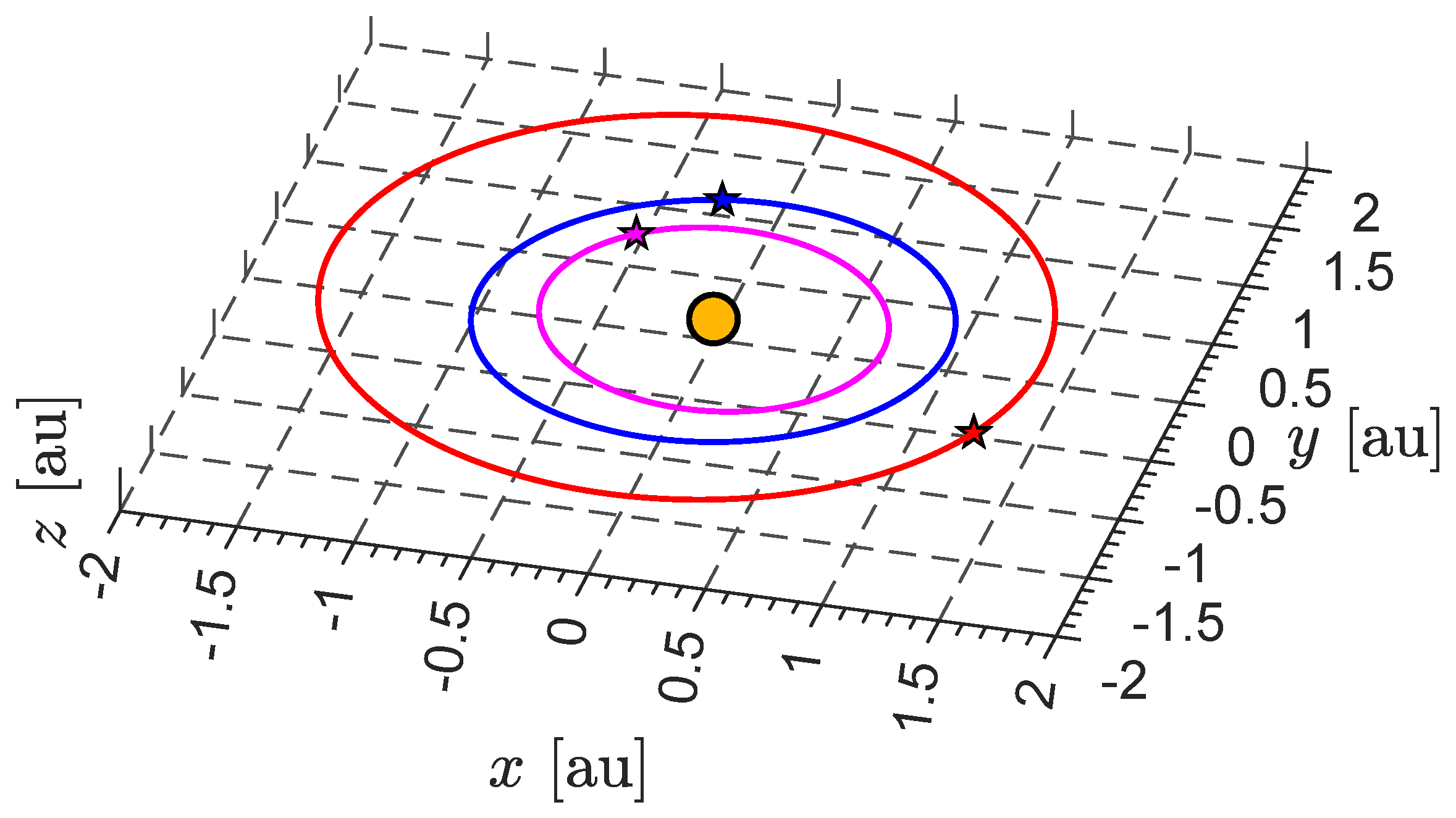
The impact on the transfer performance of a constant value of the sail pitch angle has been studied considering two typical interplanetary transfers, which model an Earth–Venus mission and an Earth–Mars mission. In particular, a three-dimensional orbit-to-orbit transfer has been considered in the study, i.e., a case where the E-sail propelled deep space probe performs the orbital transfer without considering the planetary ephemerides. This allows one to determine, as it is well known, the global optimum performance (in terms of flight time) of the assigned transfer, while simplifying the numerical analysis of the problem since it is not necessary to constrain the initial and final position of the spacecraft on the initial parking orbit (i.e., the orbit of the Earth) and on the final target orbit (i.e., that of Venus or Mars). In these two mission scenarios, the heliocentric orbital characteristics of the planets were derived from JPL’s horizons on-line ephemeris system as of 1 March 2025, as can be seen in Figure 7.

Figure 7.
Keplerian orbits of the three planets involved in the numerical analysis. Blue line → Earth; red line → Mars; magenta line → Venus; star → perihelion point; orange dot → the Sun.
In these two classical interplanetary mission scenarios, the dynamics of the spacecraft equipped with the E-sail with a fixed pitch angle were described using Walker’s equinoctial orbital elements [41,42,43], while the transfer trajectory was determined by minimizing the total flight time . For this purpose, an indirect method based on the calculus of variations [44] was employed and the procedure recently described by the author in ref. [45] was used to derive the optimal control law and the corresponding mathematical model which allows the rapid transfer trajectory to be calculated. In particular, the general procedure illustrated in ref. [45] can be adapted to the case studied in this paper by simply changing the boundary conditions related to the characteristics of the orbits of planets involved in the transfer, and exclusively considering the optimal control law related to the switching function and the sail clock angle , being in this case the value of a constant of motion. To be precise, Equations (27)–(28) and (31)–(32) of ref. [45] were used to determine the optimal control law during the transfer, while the boundary value problem was solved via a simple shooting procedure with a precision of when the equations of motion are expressed in a dimensionless form. These latter, together with the Euler–Lagrange equations [46], were numerically integrated with a precision of using a routine based on the Adams–Bashforth method [35,36].
In order to avoid very long flight times, and taking into account the geometric characteristics of the three Keplerian orbits (see Figure 7) involved in the two interplanetary transfers the sail pitch angle has been assumed in the range . The latter, according to Equation (4), corresponds to a sail cone angle included in the interval , where the upper value of the interval is equal to the maximum admissible value of the cone angle; see also Figure 4. Moreover, the interval contains the value which maximizes the transverse component of the propulsive acceleration. In other terms, the numerical simulations were obtained by considering a fixed-cone angle with a value greater than roughly . As for the characteristic acceleration, three possible values of were considered, namely , , and , which correspond, taking into account current technology, substantially to a low, medium, or high performance E-sail, respectively. Note that the case of is consistent with the scenario in which the generic transfer is performed by using an E-sail with a sort of “canonical value” of the characteristic acceleration, as defined by McInnes [29] for a photonic solar sail-based transfer. The results of numerical simulations are illustrated in the next section.
4. Numerical Simulations and Results
The first step to determine the impact on the flight time of a constrained control law that provides for the maintenance of a constant value of the sail pitch angle during the interplanetary transfer is to calculate the mission time in the classic case in which can be freely varied during the flight. This specific (reference) situation is indicated in the rest of the paper, with the subscript u. In other words, the first step is to solve an unconstrained (with regard to the sail pitch angle) minimum-time optimization problem, in order to obtain a set of reference values for the flight time to be used as a term of comparison for the results that will then be obtained in the next step, i.e., the one in which the value of will be fixed during the transfer.
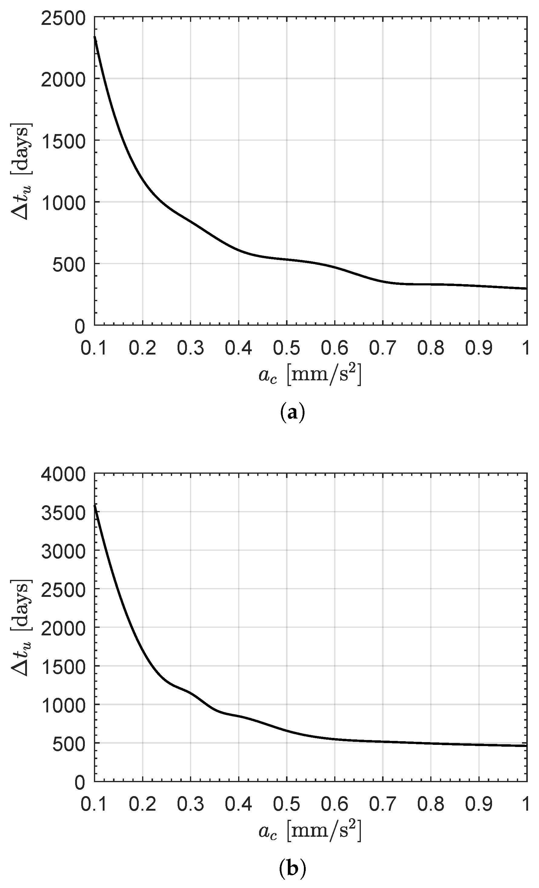
To this end, the procedure described in ref. [45] is used, leaving the sail pitch angle free to vary during the flight according to the corresponding optimal guidance law, in order to minimize the orbit-to-orbit transfer time in a given mission scenario (in this case, an Earth–Venus or an Earth–Mars) and for a given value of the spacecraft characteristic acceleration . More precisely, in this kind of unconstrained sail pitch angle-case, the control law described by Equation (30) of [45] is used for and, considering , the curves drawn in Figure 8 are obtained. In particular, the graphs in that figure describe the usual shape of the function which has a vertical asymptote when the characteristic acceleration is reduced to very small values. On the other hand, the variation (i.e., the reduction) in the optimal flight time is less marked when the propulsive performance of the E-sail increases, and the value of reaches (or exceeds) the canonical one of .

Figure 8.
Minimum flight time in an unconstrained (from the point of view of the sail pitch angle ) orbit-to-orbit interplanetary transfer as a function of the spacecraft characteristic acceleration . (a) Case of an Earth–Venus transfer; (b) Case of an Earth–Mars transfer.
Using the curves in Figure 8, it is possible to extrapolate the reference values of the minimum flight time , in the two interplanetary mission scenarios, when . The values of such flight times, which will be used to compare the results obtained in the sail pitch angle-constrained case, are summarized in Table 1.

Table 1.
Numerical value of the minimum flight time in an unconstrained (from the sail pitch angle point of view) interplanetary orbit-to-orbit transfer when .
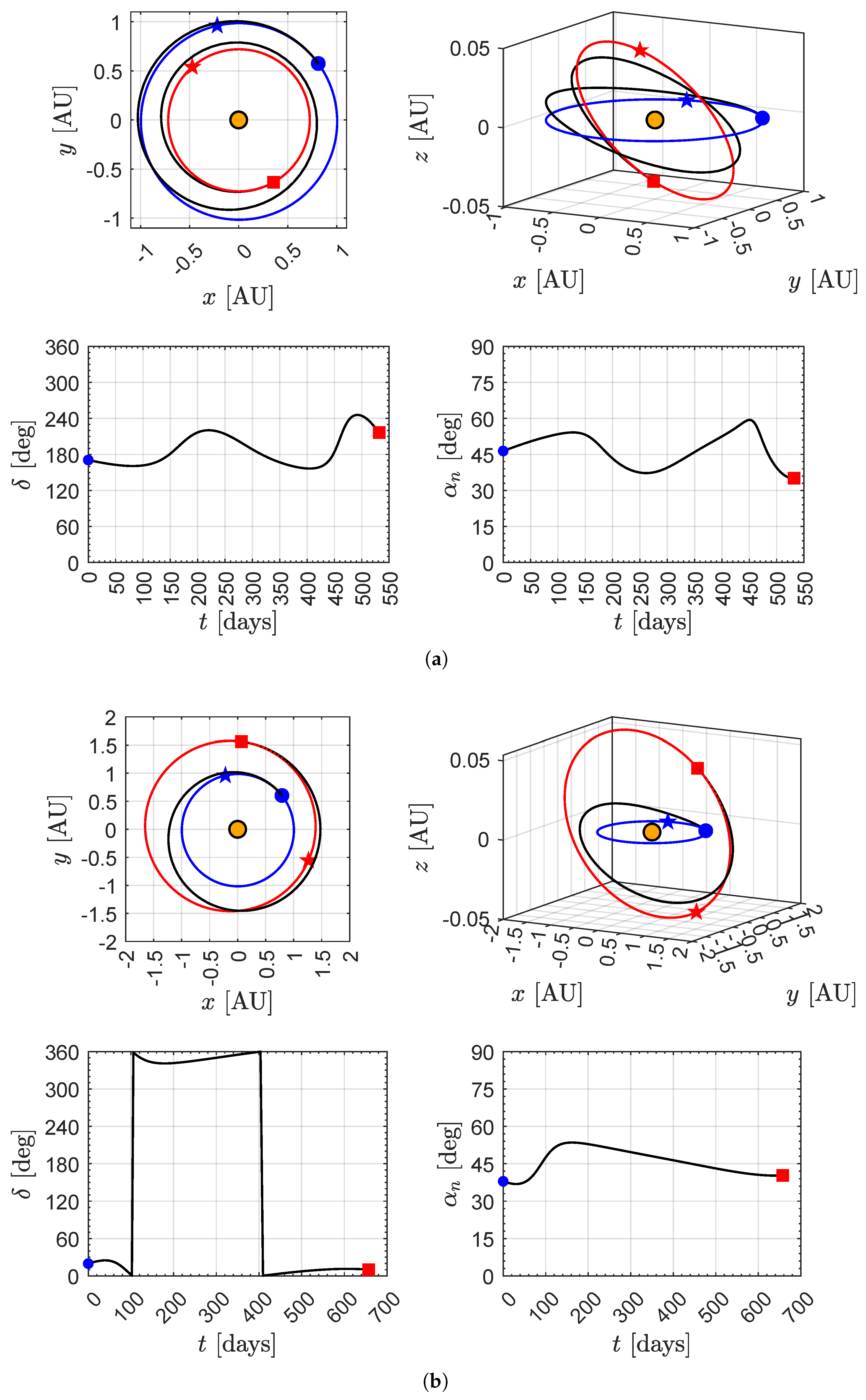
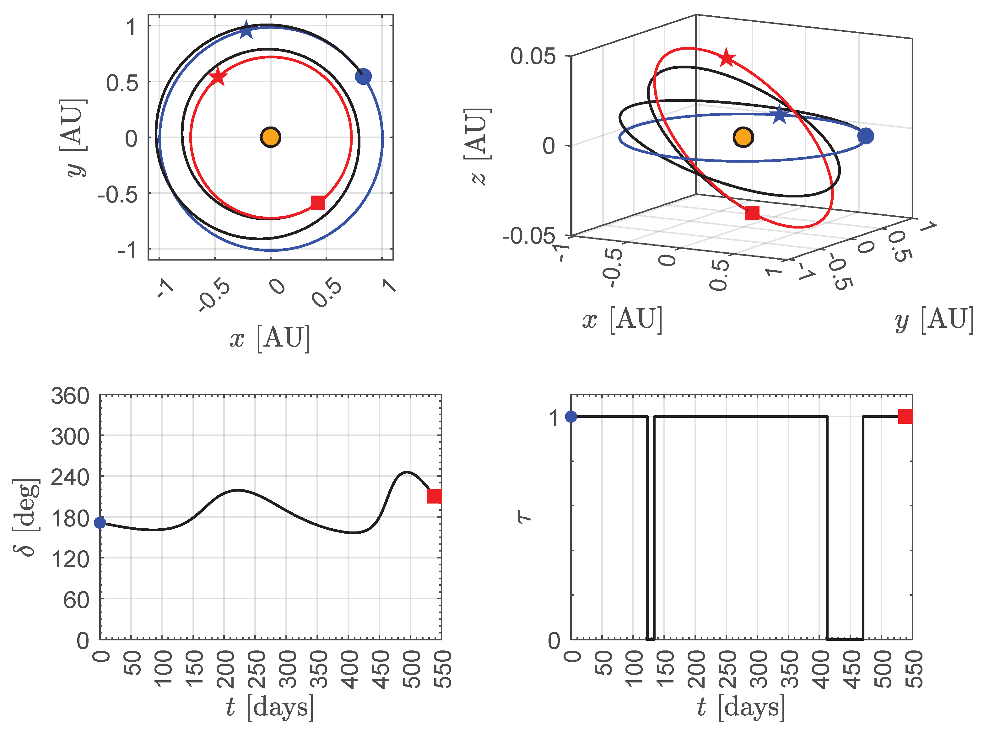
The optimal spacecraft transfer trajectory and the optimal time variation of the two control angles and in the two mission scenarios, when and the sail pitch angle is unconstrained, is reported in Figure 9. Moreover, Figure 10 and Figure 11 show the unconstrained results when and , respectively.
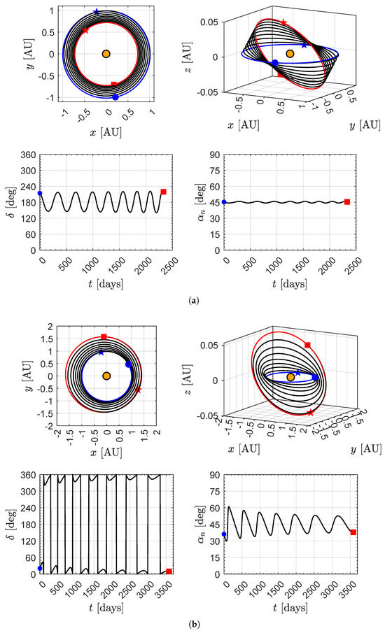
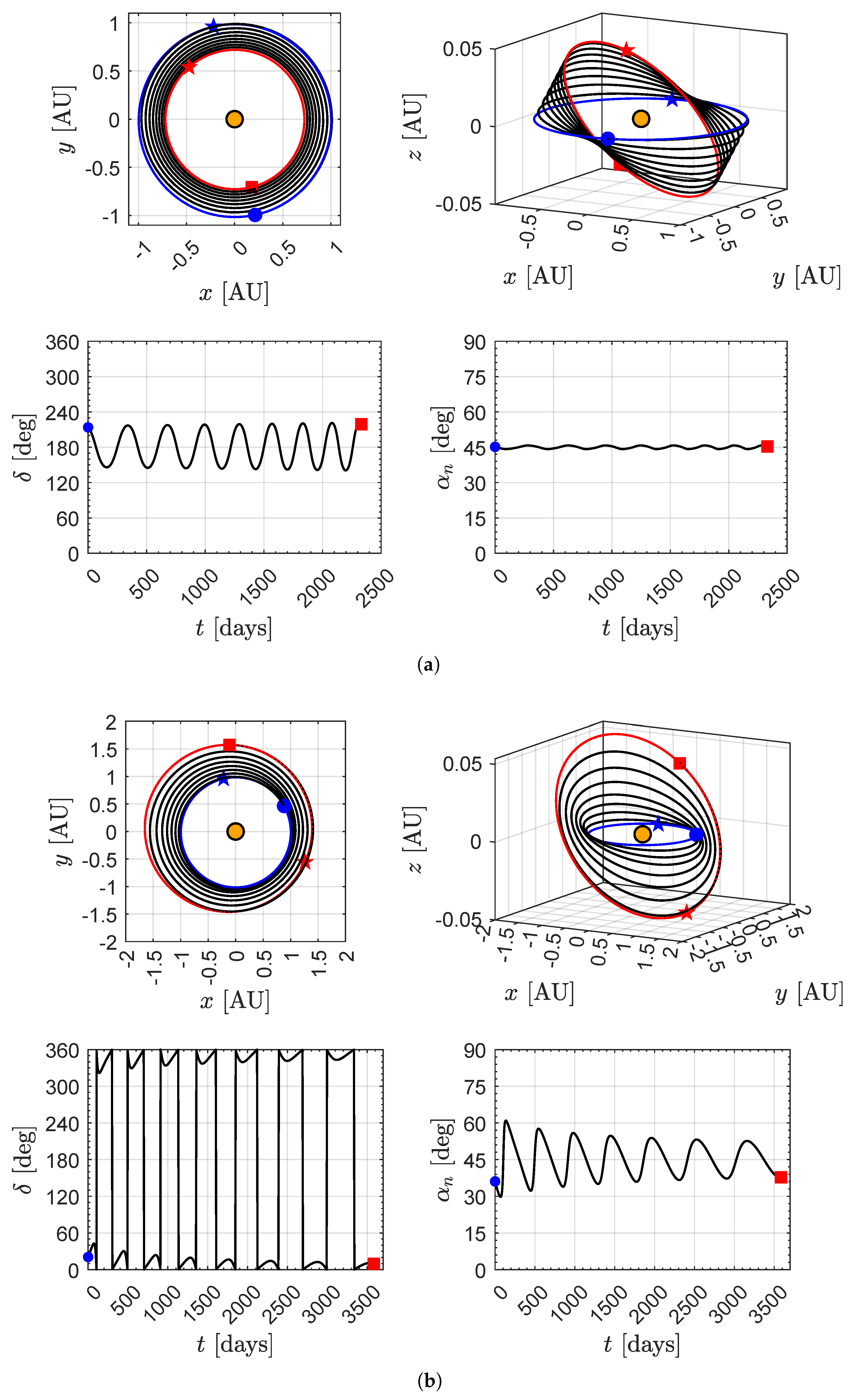
Figure 9.
Optimal spacecraft trajectory and time variation of the two control angles in an unconstrained interplanetary transfer when . Black line → spacecraft trajectory; blue line → Earth orbit; red line → target planet orbit; blue star → Earth’s perihelion point; red star → target planet’s perihelion point; orange dot → the Sun; blue dot → start; red square → arrival. (a) Case of an Earth–Venus transfer; (b) Case of an Earth–Mars transfer.
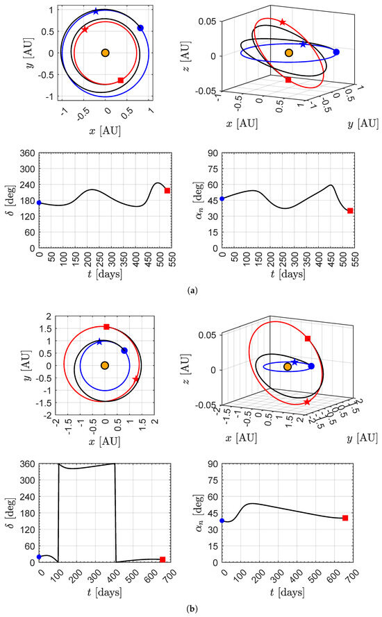
Figure 10.
Case of an unconstrained interplanetary transfer when . The legend is reported in Figure 9. (a) Case of an Earth–Venus transfer; (b) Case of an Earth–Mars transfer.
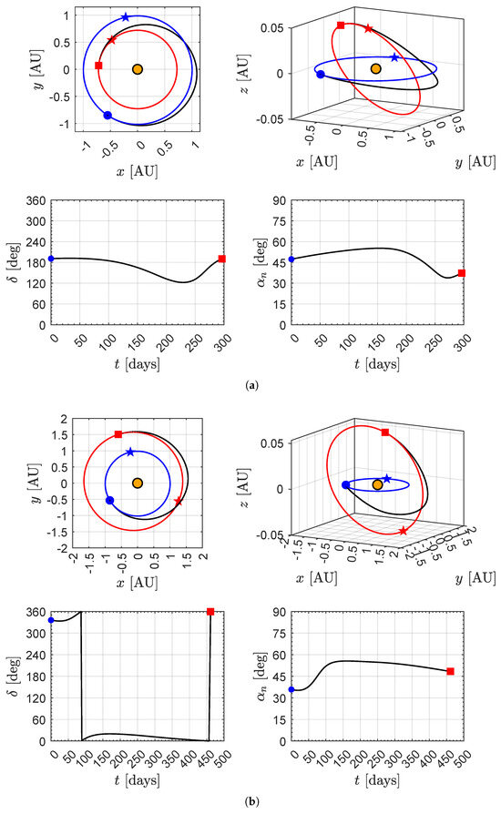
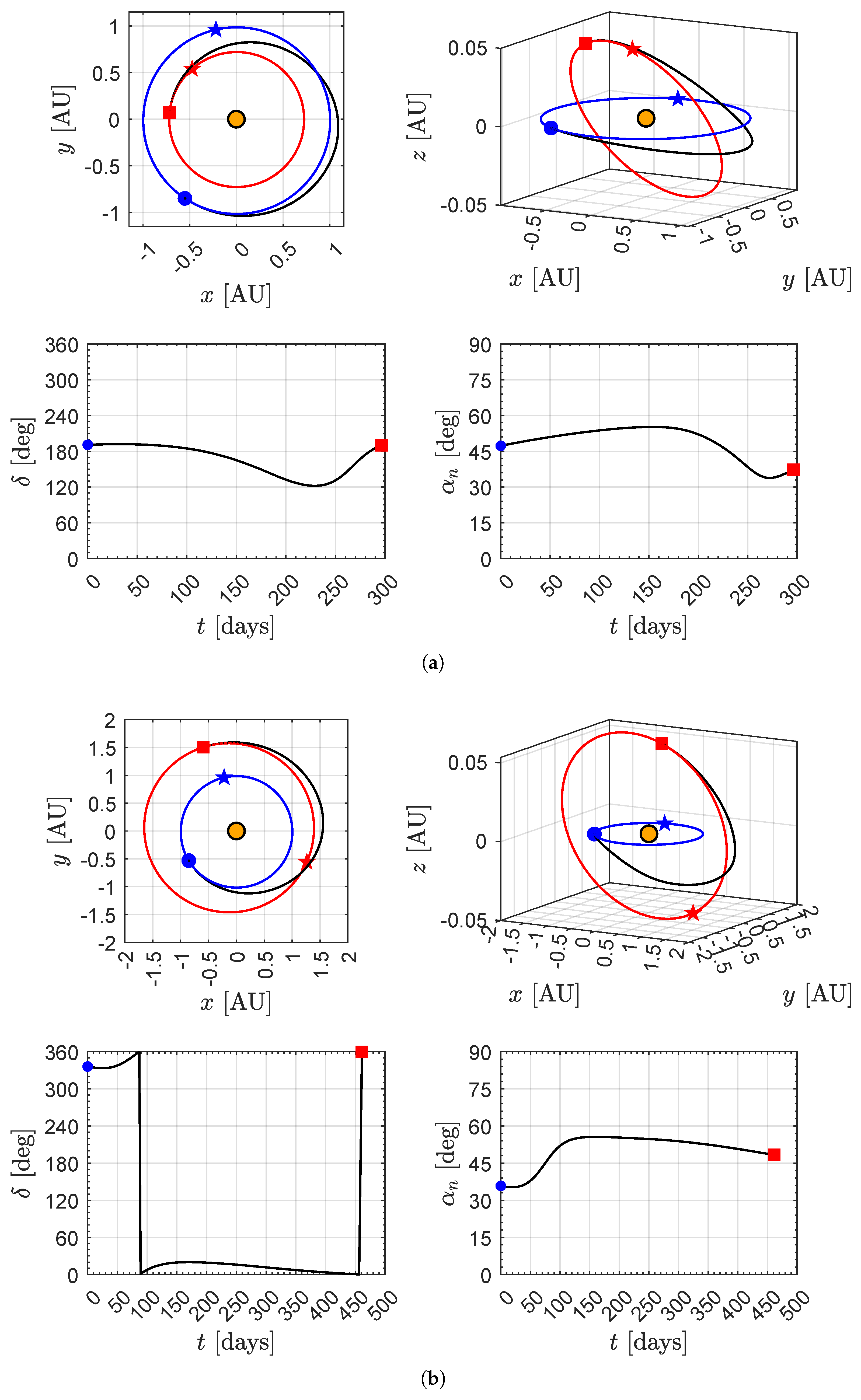
Figure 11.
Case of an unconstrained interplanetary transfer when the E-sail has a canonical value of the characteristic acceleration, i.e., . The legend is reported in Figure 9. (a) Case of an Earth–Venus transfer; (b) Case of an Earth–Mars transfer.
In particular, Figure 9 clearly indicates that, in the unconstrained case of a low-performance E-sail (i.e., for and ), the three-dimensional interplanetary transfer is performed by completing a significative number of revolutions around the Sun. This involves a continuous variation of both the two control angles and , which perform a sort of oscillatory motion around their average values. An interesting aspect that emerges from the figure is that the sail pitch angle moves, during the interplanetary flight, around the average value of that maximizes the transversal component of the propulsive acceleration (see also Figure 5) both in the case of an Earth–Mars transfer, i.e., in the case of an orbit raising, and in the case of an Earth–Venus transfer, which can be considered a sort of heliocentric orbit lowering. In these two mission scenarios, the difference is made by the value of the clock angle , which oscillates around for the Venus-based transfer, or zero for the transfer to Mars. As expected, according to Figure 10 and Figure 11, the cases of a medium or high performance E-sail, i.e., the cases where or , show a reduced number of revolutions around the Sun and a simpler optimal control law of and when compared to the case of . In any case, the mean value of the sail pitch angle remains close to , i.e., the value that maximizes even in an interplanetary transfer with a medium-high performance E-sail.
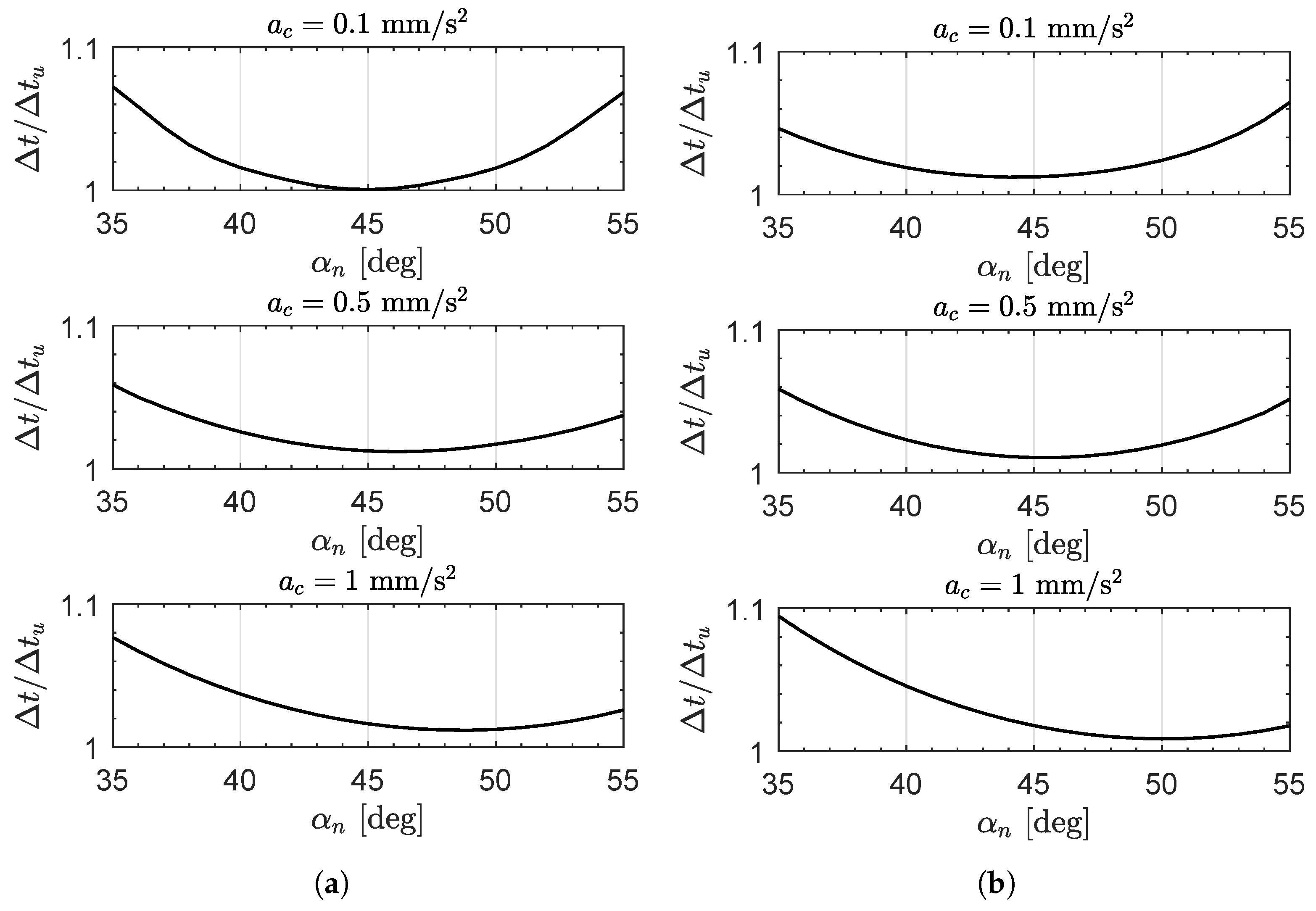
At this point, we consider an interplanetary transfer with a fixed value of the sail pitch angle, which is selected within the interval . Note that this interval substantially corresponds to taking a range of with respect to the value (precisely ) that maximizes the transversal component of propulsive acceleration; see Figure 5. The results of the optimization of the spacecraft transfer trajectory, in terms of variation of the (dimensionless) minimum flight time as a function of and , are summarized in Figure 12.
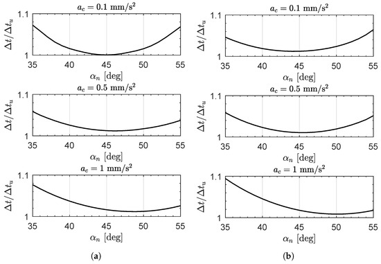
Figure 12.
Numerical results of a sail pitch angle-constrained interplanetary transfer: minimum flight time as a function of and . The value of the flight time in an unconstrained scenario is reported in Table 1. (a) Case of an Earth–Venus transfer; (b) Case of an Earth–Mars transfer.
The curves in Figure 12 clearly indicate that, in the considered range of the fixed-sail-pitch angle, the minimum flight time remains close to the value obtained in the unconstrained case. In fact, both in the Earth–Venus and Earth–Mars mission scenarios, the ratio remains well below and, in the specific case of the Earth–Venus transfer with , the difference between and is only a few days.
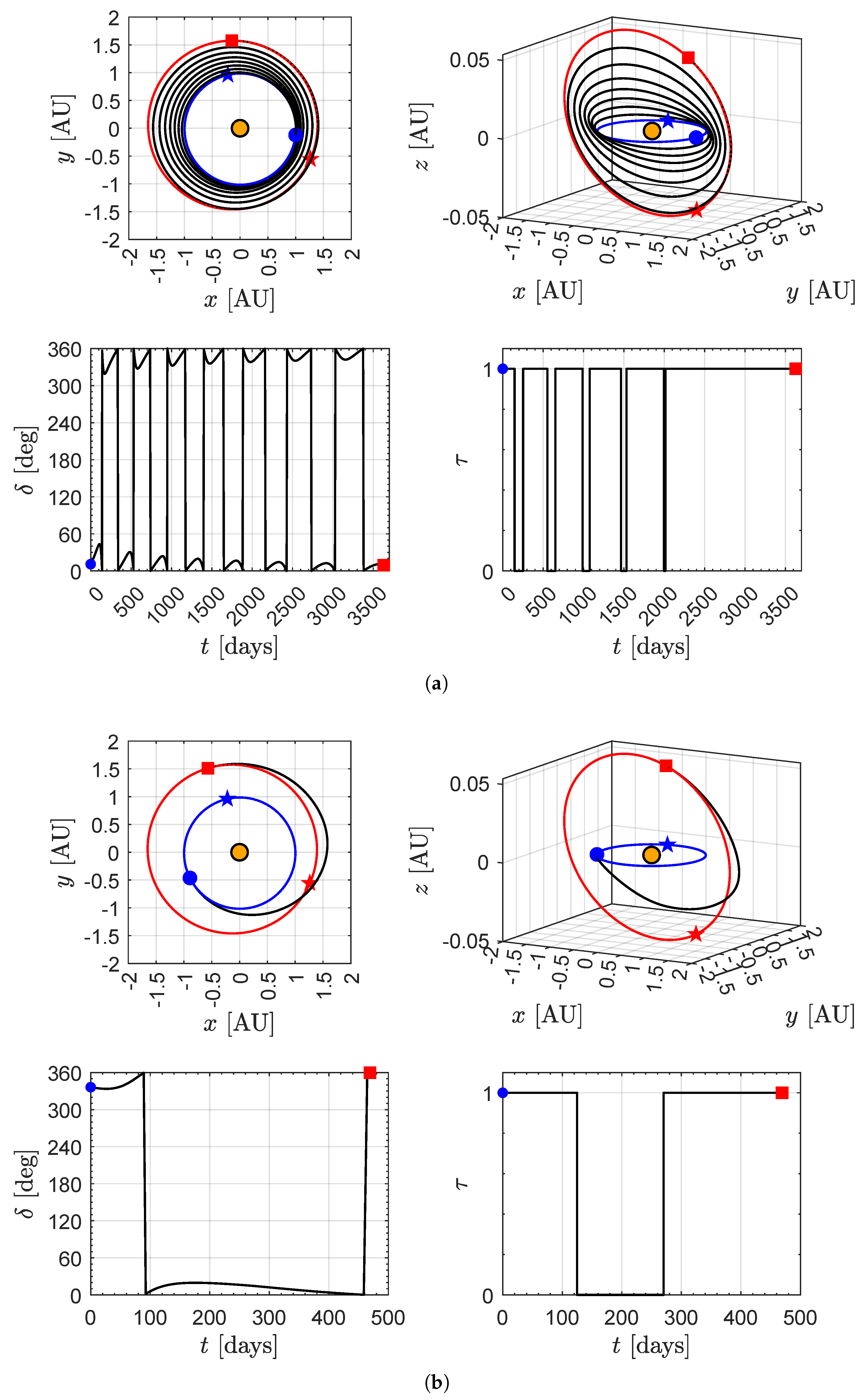
This situation occurs when the sail pitch angle has the value that maximizes the transversal component of the propulsive acceleration . Indeed, in the case of , the value of the flight time substantially reaches the value closest to the minimum admissible , especially for characteristic acceleration values compatible with a low-performance E-sail. The case of can therefore be considered as a case of particular interest in the design of an orbit-to-orbit transfer to Venus or Mars. In this regard, Figure 13 shows, for example, the optimal trajectory transfer and the time variation of the two remaining control terms and in the Earth–Mars scenario when , i.e., in the case of a low or high performance E-sail. Moreover, Figure 14 shows the case of an Earth–Venus mission when and , which confirms the possibility of performing the transfer with this specific value of the sail pitch angle.
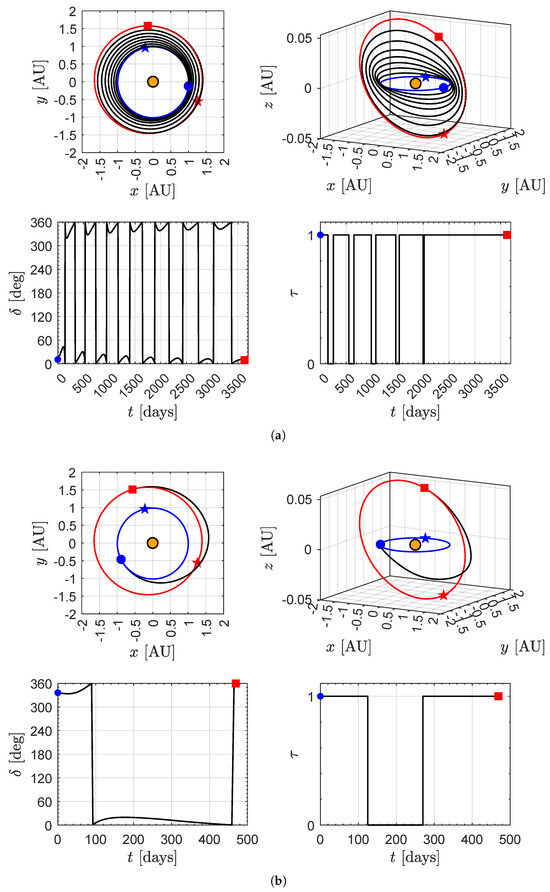
Figure 13.
Case of a constrained Earth–Mars interplanetary transfer with . The legend is reported in Figure 9. (a) Case of ; (b) Case of .
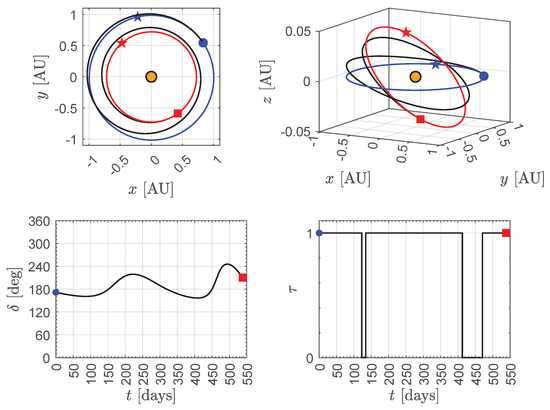
Figure 14.
Constrained Earth–Venus interplanetary transfer with and . The legend is reported in Figure 9.
Finally, Table 2 summarizes the minimum (constrained) flight times which can be obtained by solving the optimal control problem in the two interplanetary mission scenario when and . Note that the specific value of the sail pitch angle allows the designer to obtain a flight time close to the value of by using a simplified steering law, in which only the clock angle and the switching parameter change during the interplanetary transfer.
Table 2.
Minimum flight time in a constrained orbit-to-orbit interplanetary transfer with .
Interestingly, even in the sail pitch-angle constrained case, the clock angle oscillates around (or remains close to) the value of in an Earth–Venus transfer, or to the value of zero in a transfer to Mars. This aspect suggests a simplified approach to the evaluation of the optimal time of flight, which uses a two-dimensional approach and a constant setting of the E-sail in the orbital reference frame. Such a simplified semi-analytic approach, which extends the model recently proposed by the author in ref. [47] for a transfer between two close circular heliocentric orbits, can be considered as a potential extension of this work in the case of a mission towards Mars or Venus.
5. Conclusions
This paper has studied the performance of a deep space vehicle equipped with an Electric Solar Wind Sail (E-sail) in the case where the sail attitude is partially constrained during the orbital transfer between Earth and Venus or Mars. In particular, the study proposed in this paper considers a constant value of the sail pitch angle, allowing a reduced thrust vectoring of the propulsion system thanks to the variation of the clock angle. Furthermore, the presence of possible coasting arcs in the interplanetary trajectory of the spacecraft is ensured by the presence of an appropriate switching function that models the possible shutdown of the propulsion system.
The presence of the constraint on the sail pitch angle value does not substantially influence the transfer performance, if the flight time is considered as a performance index and an appropriate pitch angle value is used. In fact, the numerical simulations carried out considering three different performance levels of the E-sail, defined by three different values of the characteristic acceleration, have clearly indicated that the increase in flight time by moving from an unconstrained reference model to one in which the sail pitch angle is fixed during the flight, is rather limited and results in a few percentage points if a pitch angle of forty-five degrees is selected. This specific value of the sail pitch angle is, in fact, the one that maximizes the transversal component of the E-sail-induced propulsive acceleration vector. This aspect confirms the semi-analytical results of the recent literature which, however, were obtained considering a two-dimensional (and purely circular) model of the interplanetary transfer. In this work instead, the interplanetary orbital transfer was studied in its actual three-dimensionality, with the only simplifying hypothesis regarding the use of planetary ephemerides, in order to obtain globally optimal results from the point of view of the time of flight.
The obtained results indicate that a simplified guidance law is indeed possible for a spacecraft equipped with an E-sail, provided that the value of the sail pitch angle is appropriately selected in the assigned mission scenario. In this sense, the procedure and the model discussed in this paper can be considered an intermediate way between the classical unconstrained case in which the sail nominal plane is freely steerable and the much more stringent one, in which the inertial attitude of the E-sail propulsion system is kept fixed during the heliocentric flight.
Funding
This research received no external funding.
Institutional Review Board Statement
Not applicable.
Informed Consent Statement
Not applicable.
Data Availability Statement
The original contributions presented in the study are included in the article, further inquiries can be directed to the corresponding author.
Acknowledgments
The author declares that he has not used any kind of generative artificial intelligence in the preparation of this manuscript, nor in the creation of images, graphs, tables, or related captions.
Conflicts of Interest
The author declares no conflicts of interest.
Abbreviations and Symbols
The following abbreviations and symbols are used in this manuscript:
| Acronyms | |
| E-sail | Electric solar wind sail |
| JPL | Jet Propulsion Laboratory |
| Symbols | |
| E-sail-induced propulsive acceleration vector [mm/s2] | |
| Characteristic acceleration [mm/s2] | |
| Component of vector along [mm/s2] | |
| Component of vector along [mm/s2] | |
| Component of vector along [mm/s2] | |
| Transversal component of vector [mm/s2] | |
| Normal unit vector of | |
| Unit vector normal to the shadowed side of the sail nominal plane | |
| Radial unit vector of | |
| Spacecraft position vector [AU] | |
| Radial unit vector | |
| r | Sun–spacecraft (radial) distance [AU] |
| Reference solar distance [1 AU] | |
| Radial-transverse-normal reference frame | |
| Transverse unit vector of | |
| t | Time [days] |
| E-sail cone angle [deg] | |
| E-sail pitch angle of fixed value [deg] | |
| E-sail clock angle [deg] | |
| Total flight time [days] | |
| Dimensionless switching parameter | |
| Subscripts | |
| u | Reference, unconstrained case |
References
- Janhunen, P.; Sandroos, A. Simulation study of solar wind push on a charged wire: Basis of solar wind electric sail propulsion. Ann. Geophys. 2007, 25, 755–767. [Google Scholar] [CrossRef]
- Janhunen, P. Electric sail for spacecraft propulsion. J. Propuls. Power 2004, 20, 763–764. [Google Scholar] [CrossRef]
- Iakubivskyi, I.; Ehrpais, H.; Dalbins, J.; Oro, E.; Kulu, E.; Kütt, J.; Janhunen, P.; Slavinskis, A.; Ilbis, E.; Ploom, I.; et al. ESTCube-2 mission analysis: Plasma brake experiment for deorbiting. In Proceedings of the 67th International Astronautical Congress, Guadalajara, Mexico, 26–30 September 2016. [Google Scholar]
- Janhunen, P. Simulation study of the plasma-brake effect. Ann. Geophys. 2014, 32, 1207–1216. [Google Scholar] [CrossRef]
- Janhunen, P. Electrostatic plasma brake for deorbiting a satellite. J. Propuls. Power 2010, 26, 370–372. [Google Scholar] [CrossRef]
- Fu, B.; Sperber, E.; Eke, F. Solar sail technology—A state of the art review. Prog. Aerosp. Sci. 2016, 86, 1–19. [Google Scholar] [CrossRef]
- Gong, S.; Macdonald, M. Review on solar sail technology. Astrodynamics 2019, 3, 93–125. [Google Scholar] [CrossRef]
- Zhao, P.; Wu, C.; Li, Y. Design and application of solar sailing: A review on key technologies. Chin. J. Aeronaut. 2023, 36, 125–144. [Google Scholar] [CrossRef]
- Janhunen, P.; Toivanen, P.K.; Polkko, J.; Merikallio, S.; Salminen, P.; Haeggström, E.; Seppänen, H.; Kurppa, R.; Ukkonen, J.; Kiprich, S.; et al. Electric solar wind sail: Toward test missions. Rev. Sci. Instrum. 2010, 81, 111301. [Google Scholar] [CrossRef]
- Envall, J.; Janhunen, P.; Toivanen, P.K.; Pajusalu, M.; Ilbis, E.; Kalde, J.; Averin, M.; Kuuste, H.; Laizans, K.; Allik, V.; et al. E-sail test payload of the ESTCube-1 nanosatellite. Proc. Est. Acad. Sci. 2014, 63, 210–221. [Google Scholar] [CrossRef]
- Li, G.; Zhu, Z.H.; Du, C. Stability and control of radial deployment of electric solar wind sail. Nonlinear Dyn. 2021, 103, 481–501. [Google Scholar] [CrossRef]
- Fulton, J.; Schaub, H. Fixed-axis electric sail deployment dynamics analysis using hub-mounted momentum control. Acta Astronaut. 2018, 144, 160–170. [Google Scholar] [CrossRef]
- Fulton, J.; Schaub, H. Dynamics and control of the flexible electrostatic sail deployment. In Proceedings of the 26th AAS/AIAA Space Flight Mechanics Meeting, Napa, CA, USA, 14–18 February 2016. [Google Scholar]
- Seppänen, H.; Rauhala, T.; Kiprich, S.; Ukkonen, J.; Simonsson, M.; Kurppa, R.; Janhunen, P.; Hæggström, E. One kilometer (1 km) electric solar wind sail tether produced automatically. Rev. Sci. Instrum. 2013, 84, 095102. [Google Scholar] [CrossRef] [PubMed]
- Rauhala, T.; Seppänen, H.; Ukkonen, J.; Kiprich, S.; Maconi, G.; Janhunen, P.; Hæggström, E. Automatic 4-wire Heytether production for the electric solar wind sail. In Proceedings of the International Microelectronics Assembly and Packing Society Topical Workshop and Tabletop Exhibition on Wire Bonding, San Jose, CA, USA, 22–23 January 2013. [Google Scholar]
- Huo, M.; Jin, R.; Qi, J.; Peng, N.; Yang, L.; Wang, T.; Qi, N.; Zhu, D. Rapid optimization of continuous trajectory for multi-target exploration propelled by electric sails. Aerosp. Sci. Technol. 2022, 129, 107678. [Google Scholar] [CrossRef]
- Jin, R.; Huo, M.; Xu, Y.; Zhao, C.; Yang, L.; Qi, N. Rapid cooperative optimization of continuous trajectory for electric sails in multiple formation reconstruction scenarios. Aerosp. Sci. Technol. 2023, 140, 108385. [Google Scholar] [CrossRef]
- Du, C.; Zhu, Z.H.; Wang, C.; Li, A.; Li, T. Evaluation of E-sail parameters on central spacecraft attitude stability using a high-fidelity rigid–flexible coupling model. Astrodynamics 2024, 8, 271–284. [Google Scholar] [CrossRef]
- Pacheco-Ramos, G.; Vazquez, R.; Garcia-Vallejo, D. Optimal planning and tracking for E-sail transition between steady-states. Aerosp. Sci. Technol. 2025, 158, 109949. [Google Scholar] [CrossRef]
- Janhunen, P. Photonic spin control for solar wind electric sail. Acta Astronaut. 2013, 83, 85–90. [Google Scholar] [CrossRef]
- Toivanen, P.; Janhunen, P. Spin Plane Control and Thrust Vectoring of Electric Solar Wind Sail. J. Propuls. Power 2013, 29, 178–185. [Google Scholar] [CrossRef]
- Toivanen, P.; Janhunen, P. Thrust vectoring of an electric solar wind sail with a realistic sail shape. Acta Astronaut. 2017, 131, 145–151. [Google Scholar] [CrossRef]
- Janhunen, P.; Toivanen, P. A scheme for controlling the E-sail’s spin rate by the E-sail effect itself. In Proceedings of the Space Propulsion 2018, Seville, Spain, 14–18 May 2018. [Google Scholar]
- Janhunen, P.; Toivanen, P. TI tether ring for solving secular spinrate change problem of electric sail. arXiv 2017, arXiv:1603.05563. [Google Scholar]
- Bassetto, M.; Quarta, A.A.; Mengali, G. Thrust model and guidance scheme for single-tether E-sail with constant attitude. Aerosp. Sci. Technol. 2023, 142 Pt A, 108618. [Google Scholar] [CrossRef]
- Quarta, A.A. Three-dimensional guidance laws for spacecraft propelled by a SWIFT propulsion system. Appl. Sci. 2024, 14, 5944. [Google Scholar] [CrossRef]
- Quarta, A.A. Impact of Pitch Angle Limitation on E-sail Interplanetary Transfers. Aerospace 2024, 11, 729. [Google Scholar] [CrossRef]
- Wright, J.L. Space Sailing; Gordon and Breach Science Publishers: Philadephia, PA, USA, 1992; pp. 223–233. ISBN 978-2881248429. [Google Scholar]
- McInnes, C.R. Solar Sailing: Technology, Dynamics and Mission Applications; Springer-Praxis Series in Space Science and Technology; Springer: Berlin, Germany, 1999; pp. 46–54, 119–120. [Google Scholar] [CrossRef]
- Du, C.; Zhu, Z.H.; Wang, C.; Li, A.; Li, T. Equilibrium state of axially symmetric electric solar wind sail at arbitrary sail angles. Chin. J. Aeronaut. 2024, 37, 232–241. [Google Scholar] [CrossRef]
- Jin, R.; Huo, M.; Yang, L.; Feng, W.; Wang, T.; Fan, Z.; Qi, N. Analytical three-dimensional propulsion process of electric sail with fixed pitch angle. Aerosp. Sci. Technol. 2024, 145, 108845. [Google Scholar] [CrossRef]
- Jin, R.; Huo, M.; Xu, Y.; Yang, L.; Feng, W.; Wang, T.; Qi, N. Analytical State Approximation of Electric Sail with Fixed Pitch Angle. J. Guid. Control Dyn. 2023, 46, 2446–2454. [Google Scholar] [CrossRef]
- Jin, R.; Huo, M.; Yang, L.; Wang, T.; Fan, Z.; Qi, N. Optimal splicing of multi-segment analytical trajectories for electric sails. Aerosp. Sci. Technol. 2023, 142, 108655. [Google Scholar] [CrossRef]
- Huo, M.Y.; Mengali, G.; Quarta, A.A. Electric sail thrust model from a geometrical perspective. J. Guid. Control Dyn. 2018, 41, 735–741. [Google Scholar] [CrossRef]
- Shampine, L.F.; Reichelt, M.W. The MATLAB ODE Suite. SIAM J. Sci. Comput. 1997, 18, 1–22. [Google Scholar] [CrossRef]
- Yang, W.Y.; Cao, W.; Kim, J.; Park, K.W.; Park, H.H.; Joung, J.; Ro, J.S.; Hong, C.H.; Im, T. Applied Numerical Methods Using MATLAB; John Wiley & Sons, Inc.: Hoboken, NJ, USA, 2020; Chapters 3 and 6; pp. 158–165, 312. [Google Scholar]
- Mengali, G.; Quarta, A.A. Optimal Solar Sail Interplanetary Trajectories with Constant Cone Angle. In Advances in Solar Sailing; Macdonald, M., Ed.; Springer Praxis Books; Springer: Berlin/Heidelberg, Germany, 2014; pp. 831–850. [Google Scholar] [CrossRef]
- Boltz, F.W. Orbital Motion Under Continuous Radial Thrust. J. Guid. Control Dyn. 1991, 14, 667–670. [Google Scholar] [CrossRef]
- Kaki, S.; Akella, M.R. Spacecraft Rendezvous in Closed Keplerian Orbits Using Constant Radial Thrust Acceleration. J. Guid. Control Dyn. 2023, 46, 1112–1125. [Google Scholar] [CrossRef]
- Vedantam, M.; Kaki, S.; Akella, M. Optimal Rendezvous Trajectories Initialized with Analytical Radial Thrust Solutions. In Proceedings of the AIAA SCITECH 2024 Forum, Orlando, FL, USA, 8–12 January 2024. [Google Scholar] [CrossRef]
- Walker, M.J.H.; Ireland, B.; Owens, J. A set of modified equinoctial orbit elements. Celest. Mech. 1985, 36, 409–419. [Google Scholar] [CrossRef]
- Kechichian, J.A. Optimal low-thrust rendezvous using equinoctial orbit elements. Acta Astronaut. 1996, 38, 1–14. [Google Scholar] [CrossRef]
- Betts, J.T. Very low-thrust trajectory optimization using a direct SQP method. J. Comput. Appl. Math. 2000, 120, 27–40. [Google Scholar] [CrossRef]
- Betts, J.T. Survey of Numerical Methods for Trajectory Optimization. J. Guid. Control Dyn. 1998, 21, 193–207. [Google Scholar] [CrossRef]
- Quarta, A.A. Optimal guidance for heliocentric orbit cranking with E-sail-propelled spacecraft. Aerospace 2024, 11, 490. [Google Scholar] [CrossRef]
- Stengel, R.F. Optimal Control and Estimation; Dover Books on Mathematics; Dover Publications, Inc.: New York, NY, USA, 1994; pp. 222–254. ISBN 978-0486682006. [Google Scholar]
- Quarta, A.A. Warm start for optimal transfer between close circular orbits with first generation E-sail. Adv. Space Res. 2025, 75, 1118–1128. [Google Scholar] [CrossRef]


Disclaimer/Publisher’s Note: The statements, opinions and data contained in all publications are solely those of the individual author(s) and contributor(s) and not of MDPI and/or the editor(s). MDPI and/or the editor(s) disclaim responsibility for any injury to people or property resulting from any ideas, methods, instructions or products referred to in the content. |
© 2025 by the author. Licensee MDPI, Basel, Switzerland. This article is an open access article distributed under the terms and conditions of the Creative Commons Attribution (CC BY) license (https://creativecommons.org/licenses/by/4.0/).