Abstract
The interaction between raft foundations and soils is generally modeled with the help of linear elastic springs. The design of structural elements can only be computed when the modulus of subgrade reaction is accurately determined, which is a time-consuming process for raft foundations with relatively large sizes due to the input of many structural loads. In the present work, an approximate procedure is studied based on the relative stiffnesses of soil–foundation systems suggested by DIN—Technical Report 130. To estimate the behavior of soil–foundation systems (rigid or flexible), the limit values of relative stiffness are first determined for raft foundations on elastic soils with the stiffness moduli obtained from one-dimensional consolidation tests by using finite element analyses. Subsequently, the values of subgrade reaction moduli obtained from the FE analyses are compared and discussed with the subgrade reaction moduli determined by using the analytical method considering the relative stiffnesses of soil–foundation systems. It is shown that for a soil–foundation system with a relative stiffness ≥ 0.174, the subgrade reaction modulus obtained from the analytical method assuming a rigid system is about 1.5 to 2 times higher than that in the FE analyses. For a soil–foundation system with a relative stiffness ≤ 0.0004, the analytical method assuming a flexible system and the FE method yield a similar value of subgrade reaction modulus in the central area of the raft foundation.
1. Introduction
Due to its complexity, the interaction between raft foundations and soils is generally modeled with the help of linear elastic springs based on Winkler’s theory [1]. The spring constant is obtained from the modulus of subgrade reaction, which corresponds to the ratio of contact pressure to settlement at any given point, multiplied by the contributory area of the node it is connected to [2,3,4]. Bending moments, shear forces, and deflections on structural elements can only be computed when the modulus of subgrade reaction is accurately determined. Relatively high values of the subgrade reaction modulus lead to faulty design of structural components, while relatively low values result in a considerable increase in the required reinforcement [5,6].
Contact pressure, which is required for the determination of the settlement and thus the subgrade reaction modulus for a raft foundation, depends on the relative stiffness of the soil–foundation system, so a distinction is theoretically made between infinitely rigid and infinitely flexible foundations [6,7].
According to ACI committee [7], the behavior of a soil–foundation system can be estimated with the help of the rigidity factor , calculated using Equation (1). The system can be assumed rigid for a value of > 0.5 and flexible for < 0.5:
where is Young’s modulus of the structure material, E is Young’s modulus of the soil, B is the foundation width, and is the moment of inertia of the structure per unit length at right angles to B.
Ignoring the effect of the superstructure, DIN—Technical Report 130 [8] suggests Equation (2) to determine the relative stiffnesses of soil–foundation systems. Theoretically, a foundation behaves as infinitely rigid for K-values >> 0 and infinitely flexible for K-values ≈ 0:
where Ef is the Young’s modulus of the foundation material, E is the Young’s modulus of the soil, and d and L are the foundation thickness and length, respectively.
According to Bergmeister and Wörner [9], the system can be considered rigid for K-values > 0.1, semi-rigid for 0.01 < K < 0.1, semi-flexible for 0.001 < K < 0.01, and flexible for K-values < 0.001:
Further equations and limit values to estimate the foundation rigidity can be found in the literature [10,11].
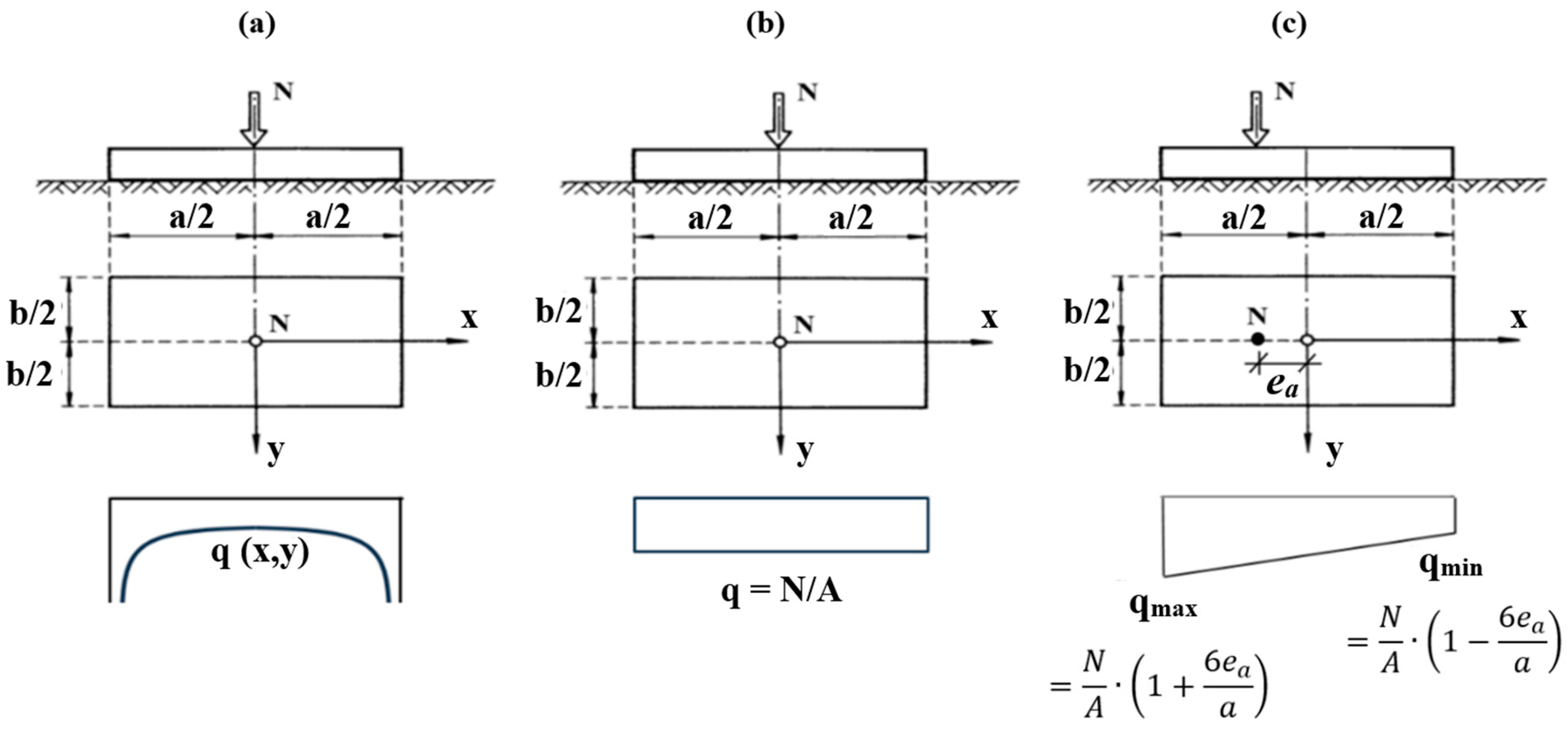
In an infinitely rigid foundation with a centrally acting axial load on an elastic half-space, the contact pressure q can be calculated using Equation (3) [12]:
where N is the axial load acting centrally, x and y are the coordinates of any point where the contact pressure q (x,y) is calculated, and a and b are foundation length and width, respectively.
As shown in Figure 1a, infinitely large pressures appear at the edges of the foundation. However, these large pressures are reduced to finite values through the development of plastic soil deformations, which leads to an increase in the contact pressure at the central zone of the foundation. As a result, a uniform contact pressure corresponding to the ratio of the axial load to the foundation area N/A can be used for infinitely rigid foundations (Figure 1b). Assuming a straight-line distribution of soil pressure, the maximum and minimum soil pressures developing under eccentrically acting axial loads can be calculated from the formula provided in Figure 1c.
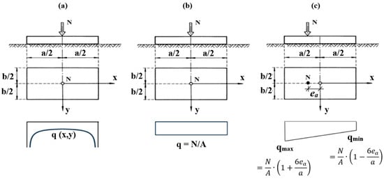
Figure 1.
Contact pressure for infinitely rigid foundations (a) resulting from a centrally acting axial load on an elastic half-space, (b) resulting from a centrally acting axial load on an elastoplastic half-space, and (c) resulting from an eccentrically acting axial load on an elastoplastic half-space.
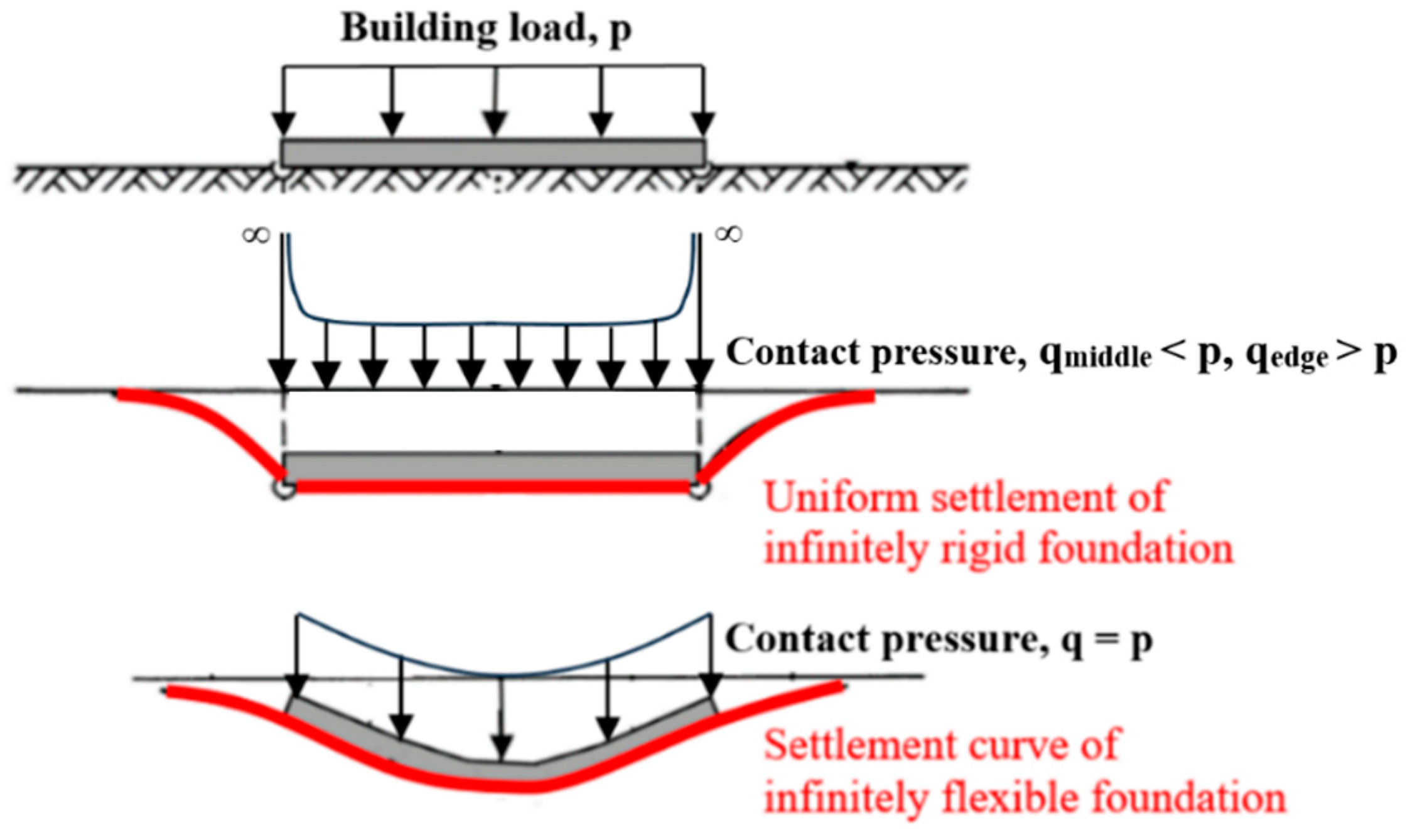
Infinitely flexible foundations have no bending stiffness and thus can freely adapt to soil deformations, so contact pressures correspond to column and wall loads. However, infinitely rigid foundations cannot follow soil deformations due to their infinitely high bending stiffnesses. As a result, the modulus of subgrade reaction has a constant value for the infinitely rigid foundation, while it varies over the contact area between the infinitely flexible foundation and the soil. The settlement profiles of infinitely rigid and flexible foundations with a uniformly distributed load on an elastic half-space are demonstrated in Figure 2.

Figure 2.
Settlement profiles of infinitely rigid and infinitely flexible foundations on an elastic half-space.
However, no system is infinitely flexible or rigid due to the interaction developed between the soil and the foundation. In the literature, various equations can be found to estimate the modulus of subgrade reaction [2,13,14,15,16]. However, these equations do not consider the effect of soil stratification, the irregularities in the foundation shape, or the irregularities in the load distribution on the modulus of subgrade reaction, so they are insufficient to obtain satisfactory results for many cases in construction practice.
In recent studies, Lee et al. [17] introduced a new analytical method reflecting the flexibility of mat foundation and the soil–spring coupling effect. Jeong et al. [18] showed, with the help of numerical analyses, that the distribution of the subgrade reaction modulus is non-uniform, so its value at the corners and edges of the mat foundation is higher than that at the center. Loukidis and Tamiolakis [19] proposed an equation describing the spatial distribution of spring stiffness based on the results of three-dimensional finite element analyses of slabs resting on elastic soil. Son et al. [20] derived an equation to estimate the scale effect on loading plates with diameters of less than 762 mm. Roy and Deb [21] performed plate load tests on layered soils with and without geogrid reinforcement. The results of these tests indicated that the interface effect reduces the subgrade reaction modulus, which appears when the spacing between the plates is less than 1.33 times the plate width. Hamza et al. [22] stated, with the help of 3D-numerical analyses, that the interface effect can be ignored when the spacing between the foundations becomes larger than three times the foundation width. Rahgooy et al. [23] studied the distribution of the subgrade reaction modulus using an elastic–perfectly plastic constitutive model. Their work indicated that the subgrade reaction moduli developing under elastic loads decrease from the corner to the center of foundation, while they increase from the corner to the center under the ultimate load. Dehghanbanadaki et al. [24] developed a novel prediction model to estimate the subgrade reaction modulus in soft soils improved with floating deep cement mixing columns. Chang et al. [25] indicated with the help of numerical analyses and the Mohr–Coulomb soil model that the modulus of subgrade reaction is strongly affected by the relative rigidity of the foundation depending on the soil stiffness and foundation dimensions. Based on the results of plate load tests and FE analyses, Lie et al. [26] stated that the subgrade reaction modulus for foundations in gravelly soils can be estimated using Terzaghi’s extrapolation method as in clayey soils.
In the present work, an approximate procedure is studied based on the relative stiffnesses of soil–foundation systems suggested by DIN—Technical Report 130. To estimate the behavior of soil–foundation systems (rigid or flexible), the limit values of relative stiffness are first determined for raft foundations on elastic soils with the stiffness moduli obtained from one-dimensional consolidation tests by using the finite element analyses. Subsequently, the values of subgrade reaction moduli obtained from the FE analyses are compared and discussed with the subgrade reaction moduli determined by using the conventional analytical method considering the system behavior. These comparisons are also conducted for the four case studies, in which asymmetrical shapes of foundations and asymmetrical distributions of structural loads are considered. The analytical method considering the system behavior enables engineers to estimate the subgrade reaction modulus in the pre-design phase without the input of many structural loads.
2. Materials and Methods
2.1. Determination of Subgrade Reaction Modulus Considering the Soil–Foundation Interaction
The soil–foundation interaction is considered using the finite element software GGU-Slab, Version 12.04 [27], which requires an iteration process for the numerical solution. The finite element mesh consists of isosceles right triangle elements with a congruent side length of 0.5 m.
In the first step of FE analyses, the settlements (elastic and primary consolidation settlements) in an elastic–isotropic soil at all nodes of the finite element mesh resulting from a contact pressure of 1 kN/m2 are calculated. For this purpose, Boussinesq’s equation [28] is numerically integrated, and the contact pressure (1 kN/m2) is divided by the calculated settlements to determine the distribution of subgrade reaction modulus for each node. Subsequently, the foundation bending is calculated based on Equation (4), which is solved using the finite element method. Finally, the subgrade reaction modulus is varied in further iteration steps until the foundation’s bending corresponds to the soil settlement.
where s is the settlement, d is the foundation thickness, Ef and νf are the Young’s modulus and the Poisson’s ratio of foundation material, q is the contact pressure, and k is the modulus of subgrade reaction.
For example, a mesh comprising 512 triangles and 289 nodes requires 147,968 settlement calculations. To limit the computational effort, a maximum settlement calculation distance of 50 m is inputted in the software. This distance ensures that settlements at the system node are only determined from triangles whose centroids are at a smaller distance from this system node. The end of the iteration is defined using a failure criteria displacement. If the difference between the foundation displacement and the soil settlement is smaller than the specified value, which has a default value of 10−5 m, at all points of the FE mesh, the analysis is stopped. The program recalculates the subgrade reaction moduli for the next iteration step from the quotients of the pressure at the node and the settlement after every iteration step. In complicated systems, this can lead to oscillations around the actual solution, so the calculation does not converge. In this case, a “damping” can be specified. The default value of 0.2 has provided good results [27].
2.2. Soil Model
The software GGU-Slab, Version 12.04 [27] uses a linear–elastic and isotropic soil model with the stiffness modulus of soil Es ( determined from the one-dimensional consolidation test for any particular pressure range and axial strain range .
The stiffness modulus of the soil was varied as 2.5, 10, 40, and 160 MPa. A constant unit weight of γ = 19 kN/m3 and Poisson’s ratio ν = 0.3 were assigned to the soil used in the numerical models.
The relationship between the stiffness modulus and the Young’s modulus of the soil can be obtained by using Hooke’s law and the boundary conditions in the one-dimensional consolidation test, as given in Equation (5):
where E and ν are the Young’s modulus and Poisson’s ratio of the soil, respectively.
The German standard for geotechnical design limits the thickness of the compressible soil layer at a depth, where the stress resulting from the contact pressure becomes less than 20% of the overburden stress. It is called the depth of settlement effect, and the settlement calculation is performed for the soil layer between the foundation base and this depth. Accordingly, the thickness of the homogeneous soil layers in the present study was chosen as 20 m, which was deeper than the depth of settlement effect.
2.3. Properties of Foundations
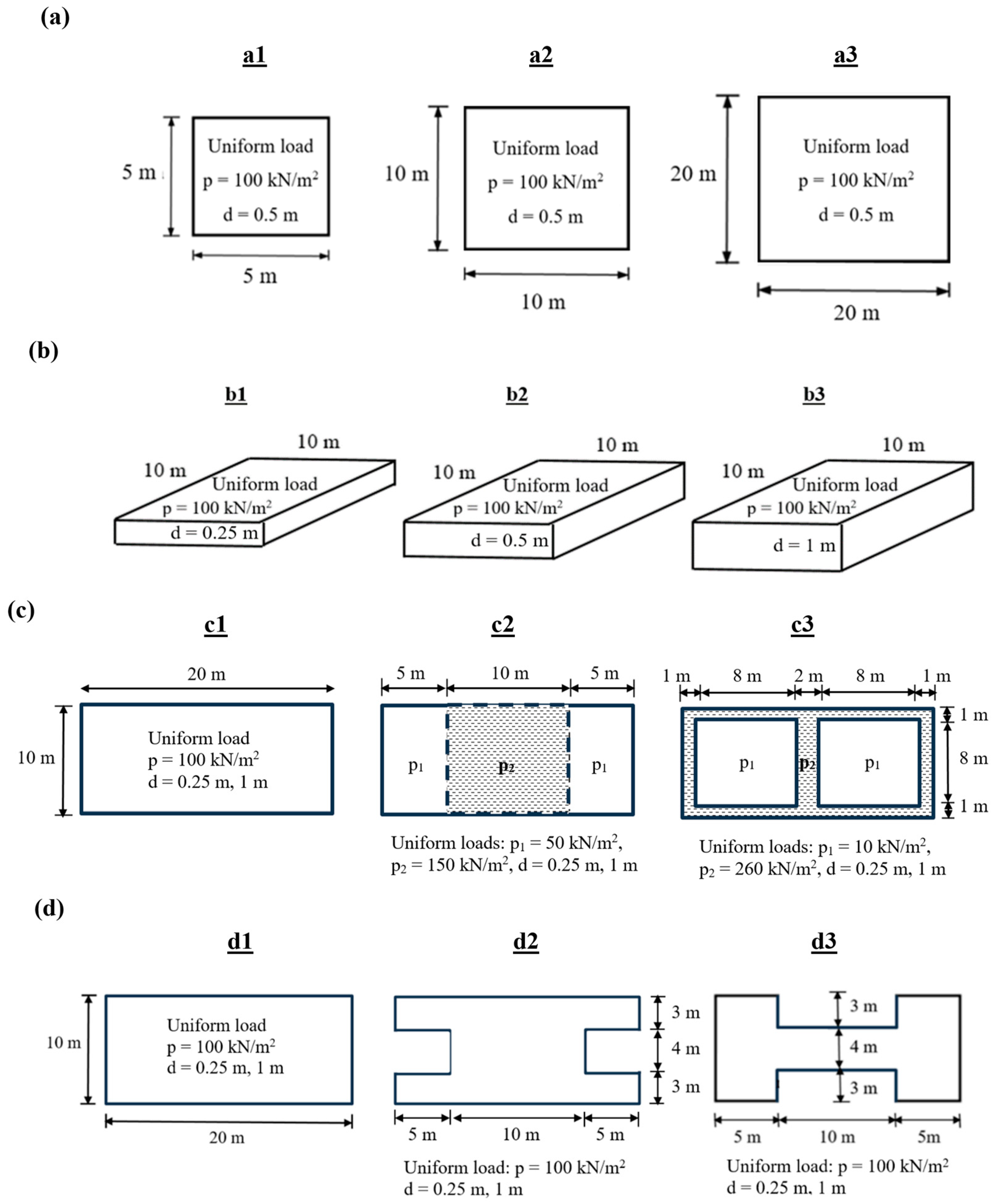
The analyses were performed for 18 foundations concerning the geometry and structure loads. The same values of Young’s modulus Ef = 31,000 MPa, Poisson’s ratio νf = 0.2, and the unit weight γf = 25 kN/m3 were assigned to the foundation material. The foundations shown in Figure 3 can be classified into four groups:
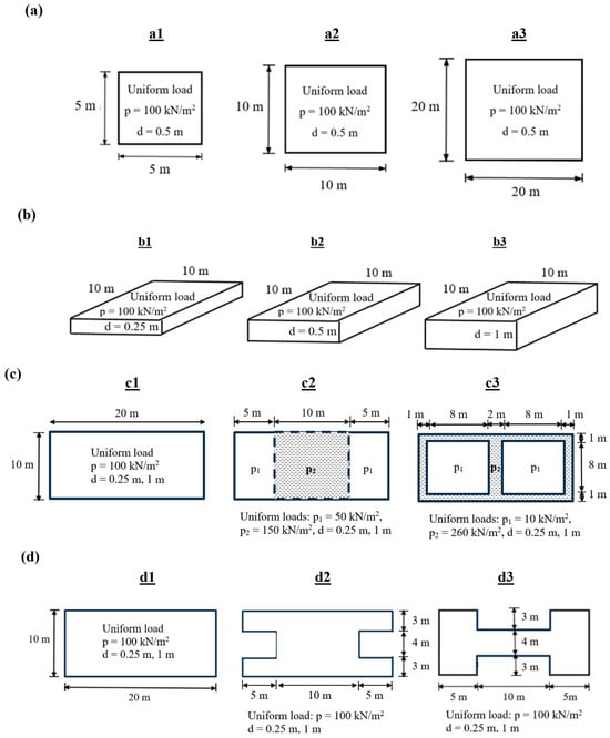
Figure 3.
Foundations examined in the numerical analyses: (a) square-shaped foundations with varying side lengths, (b) square-shaped foundations with varying thicknesses, (c) rectangular-shaped foundations with varying load distributions and thicknesses, and (d) foundations with varying shapes and thicknesses.
In the first group, the square-shaped foundations with different sizes (5 m × 5 m, 10 m × 10 m, and 20 m × 20 m) were studied (Figure 3a). All three foundations had the same thickness of d = 0.5 m, and they were loaded with a uniformly distributed load of p = 100 kN/m2. The relative stiffnesses of these soil–foundation systems were calculated according to Equation (2) and listed in Table 1.

Table 1.
Relative stiffnesses of the soil–foundation systems shown in Figure 3a.
In the second group of foundations, shown in Figure 3b, the distributions of the subgrade reaction moduli were determined for the square-shaped foundations with different thicknesses (d = 0.25, 0.5, and 1 m). All three foundations had the same side length of 10 m and were loaded with a uniformly distributed load of p = 100 kN/m2. The relative stiffnesses of these soil–foundation systems are provided in Table 2.
Table 2.
Relative stiffnesses of the soil–foundation systems shown in Figure 3b.
The effect of load distributions on the subgrade reaction modulus was examined by using a rectangular foundation (10 m × 20 m) with two different thicknesses (d = 0.25 m and 1 m) in the third group (Figure 3c). The uniformly distributed loads (p1 and p2) on foundations c2 and c3 were chosen such that no eccentricity appeared, so the total load on both foundations had the same value (20,000 kN) as on foundation c1.
In the last group (Figure 3d), the differently shaped foundations with two different thicknesses (d = 0.25 m and 1 m) were loaded with a uniformly distributed load of p = 100 kN/m2.
The relative stiffnesses of the soil–foundation systems in Figure 3c,d can be taken from Table 3 for d = 1.0 m and 0.25 m. It should be noted that foundations c2 and c3 have varying cross-sections, so the equation suggested by DIN—Technical Report 130 [8] cannot be directly applied to these foundations. Thus, the largest size of this foundation was used as L in Equation (2).
Table 3.
Relative stiffnesses of the soil–foundation systems shown in Figure 3c,d.
3. Results and Discussion
3.1. FE Analyses
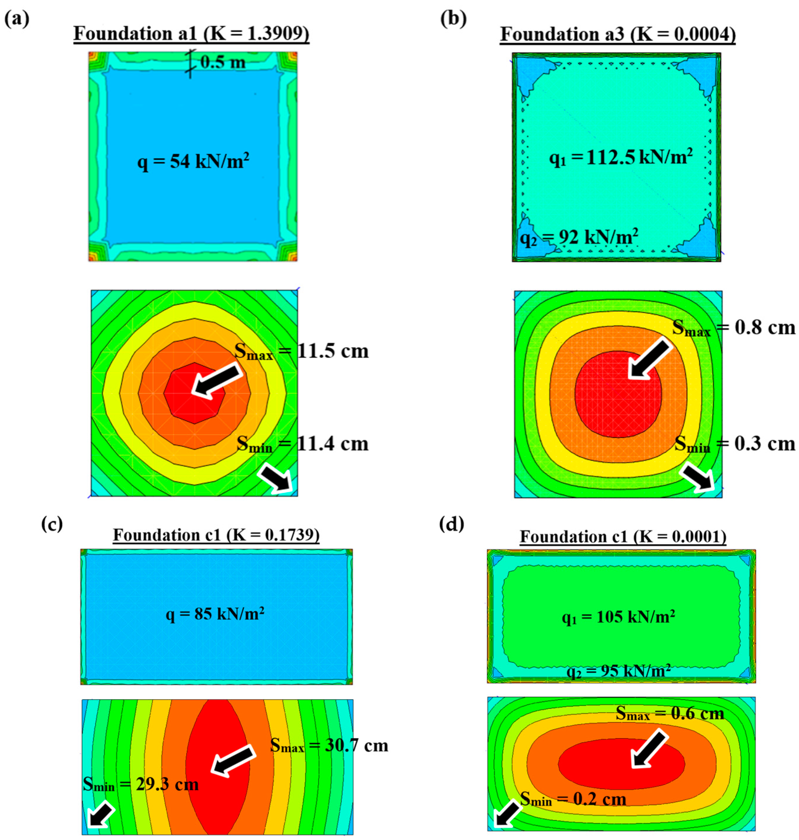
This section provides the results of a total of 72 finite element analyses. For example, the settlements S, which consist of elastic and primary consolidation settlements, and the contact pressures q obtained from these analyses are illustrated in Figure 4, Figure 5 and Figure 6 for the flexible and rigid systems according to Ref. [9].
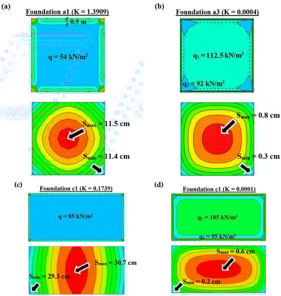
Figure 4.
The values of contact pressure q and settlement S for square- and rectangular-shaped foundations with a single uniformly distributed load: (a) foundation a1, with K = 1.3909; (b) foundation a3, with K = 0.0004; (c) foundation c1, with K = 0.1739; and (d) foundation c1, with K = 0.0001.
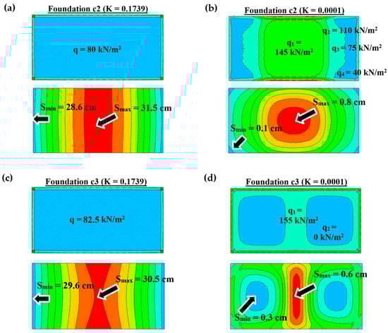
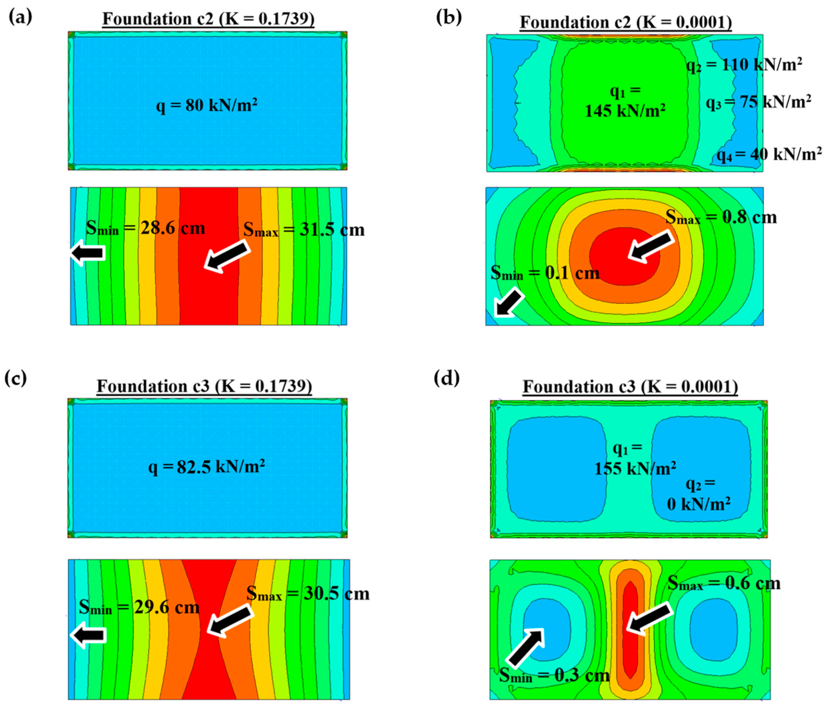
Figure 5.
The values of contact pressure q and settlement S for rectangular-shaped foundations with two uniformly distributed loads: (a) foundation c2, with K = 0.1739; (b) foundation c2, with K = 0.0001; (c) foundation c3, with K = 0.1739; and (d) foundation c3, with K = 0.0001.
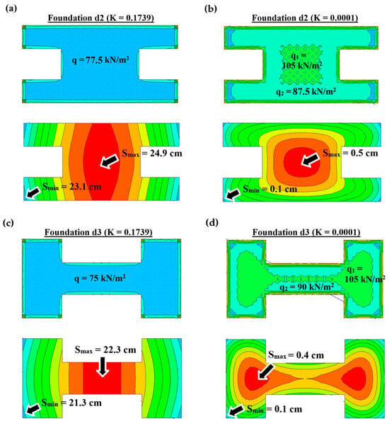
Figure 6.
The values of contact pressure q and settlement S for foundations with cross-sections with varying widths and a single uniformly distributed load: (a) foundation d2, with K = 0.1739; (b) foundation d2, with K = 0.0001; (c) foundation d3, with K = 0.1739; and (d) foundation d3, with and K = 0.0001.
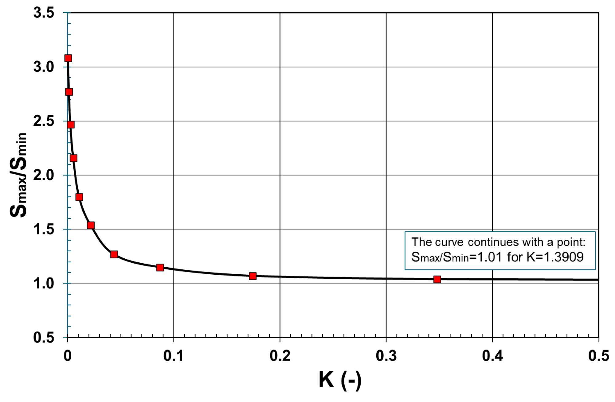
As shown in Figure 2, the uniformly distributed foundation load corresponds to the contact pressure in infinitely flexible systems, while a uniform settlement develops in infinitely rigid systems. Accordingly, the ratios of the maximal settlements to minimal settlements Smax/Smin were relatively low for the rigid systems examined in this section.
For the foundation a1 with a relative stiffness of K = 1.3909, which is classified as rigid according to Ref. [9], the ratio of Smax/Smin is equal to 1.01 (Figure 4a). For the other rigid systems with K = 0.1739 (Figure 4c, Figure 5a,c and Figure 6a,c), this ratio was higher than 1.01 due to the relatively low K-value, so it varied between 1.03 and 1.10. The varying ratios of Smax/Smin for the same value of K can be explained by the effect of foundation geometry and load distribution on the soil settlement.
Under a uniformly distributed load of 100 kN/m2, two stress zones occurred in the flexible cases with K = 0.0004 and 0.0001. The average values of the contact pressures (q1 and q2), which had a maximum deviation of 12.5% from the foundation load, are illustrated in Figure 4b,d and Figure 6b,d. The relatively high derivations that appeared in the foundations shown in Figure 5b,d are explained by the effect of load distribution on the contact pressure, because these foundations had two uniformly distributed loads in contrast to the other foundations (Figure 3c).
It should be noted that a pressure concentration developed on the edges of all soil-foundation systems examined. The pressure concentrations in the rigid systems were higher than those in the flexible systems, in accordance with Equation (3). The width of the zones with relatively high pressures was equal to 0.5 m, which corresponded to the side length of the triangle elements in the finite element mesh generated in the numerical models.
In Figure 7, Figure 8 and Figure 9, the ratios of the maximal settlements to minimal settlements Smax/Smin are provided depending on the relative stiffnesses of soil–foundation systems K. It can be seen from Figure 7, Figure 8a, and Figure 9a that the ratio of Smax/Smin is lower than 1.1 when the value of K is higher than 0.174. That means that a value of K higher than 0.1, as suggested by [9], is not satisfactory for assuming the soil–foundation system as rigid. Based on the relatively low values of K in Figure 8b and Figure 9b, the ratios of Smax/Smin are relatively high (>1.5).
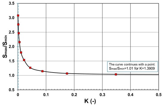
Figure 7.
Ratio of max. settlement to min. settlement for foundations a1 to a3 and b1 to b3 depending on the relative stiffnesses of the soil–foundation systems.
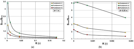
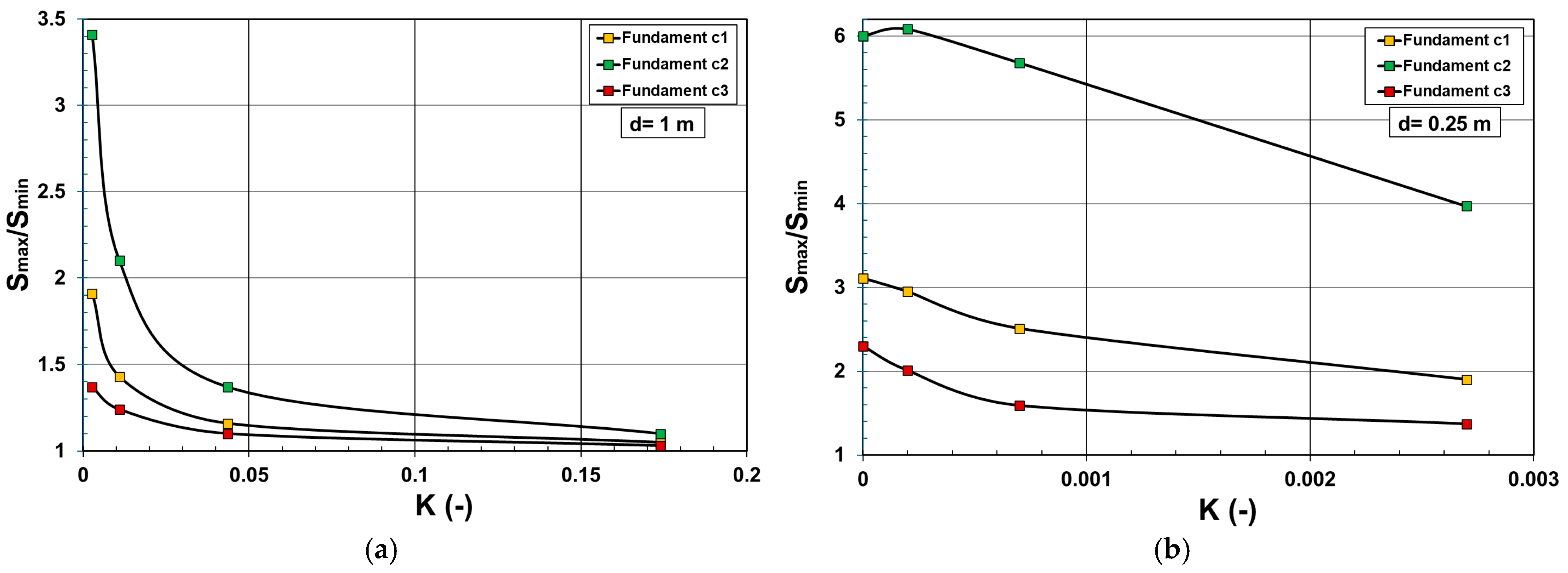
Figure 8.
Ratio of max. settlement to min. settlement for foundations c1 to c3 depending on the relative stiffnesses of the soil–foundation systems: (a) foundation thickness = 1 m; (b) foundation thickness = 0.25 m.
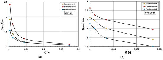
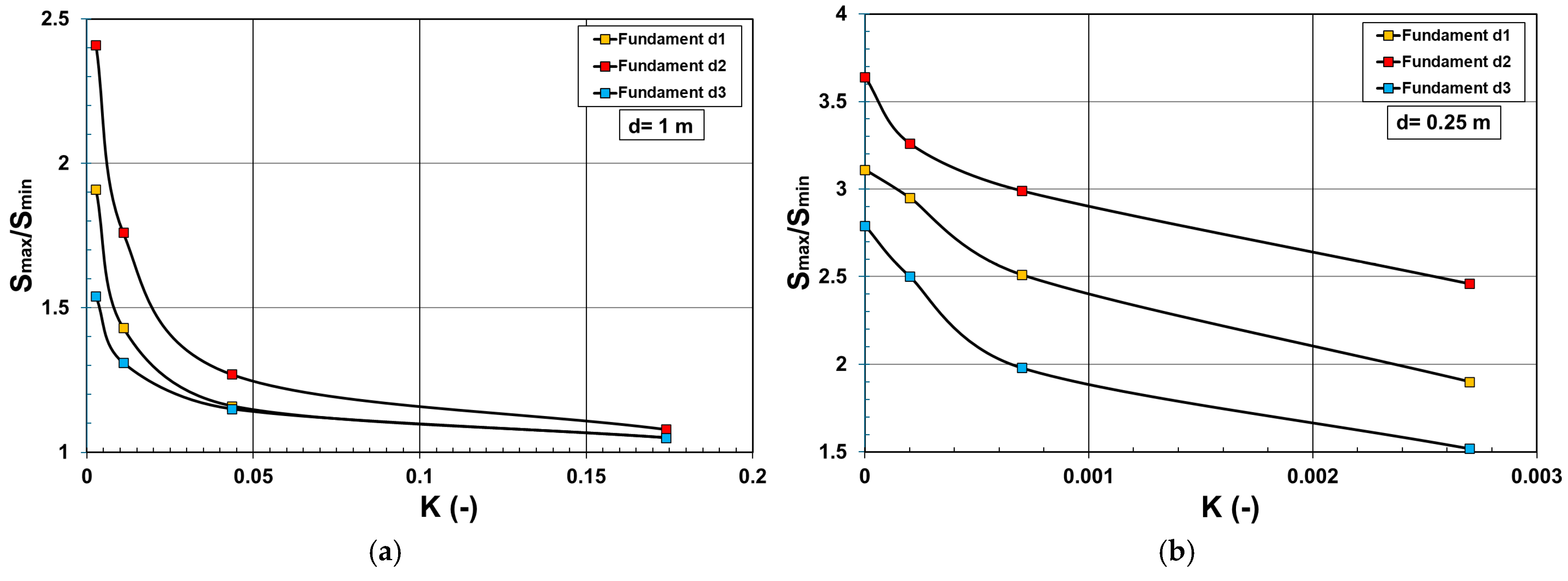
Figure 9.
Ratio of max. settlement to min. settlement for foundations d1 to d3 depending on the relative stiffnesses of the soil–foundation systems: (a) foundation thickness = 1 m; (b) foundation thickness = 0.25 m.
Here, it should be noted that the relatively low value of Smax/Smin = 1.2 for the foundation c3 with K = 0.0027 in Figure 8b results from the fact that this foundation is loaded with a relatively high uniform load of 260 kN/m2 on its edges and with a lower uniform load of 10 kN/m2 in its central area, which led to settlements at a similar magnitude.
The ratios of the foundation load to the contact pressure qload/qcontact are provided depending on the K-values in Figure 10 and Figure 11. Here, qcontact corresponded to the average value of contact pressures in the central area of the foundation, so the relatively high pressures developing on the edge zones with a width of 0.5 m were ignored.
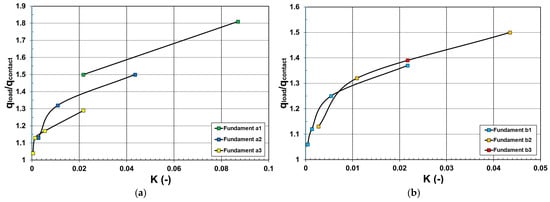
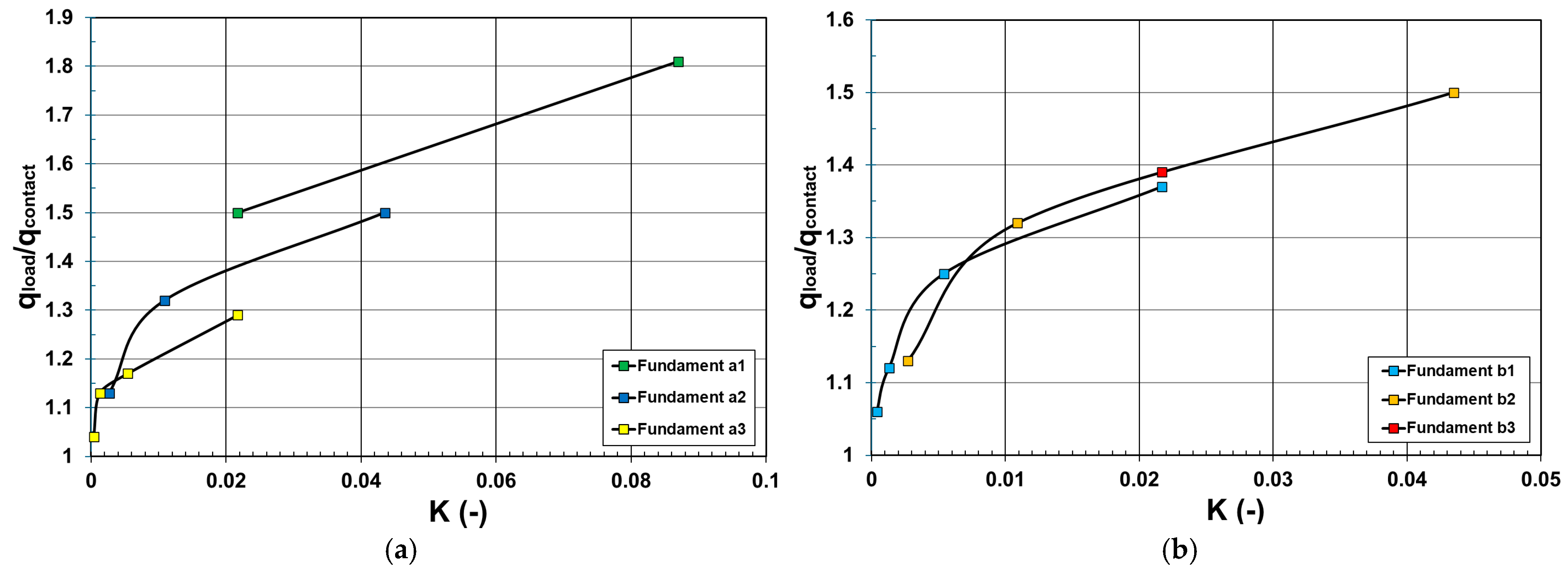
Figure 10.
Ratio of foundation load to contact pressure depending on the relative stiffnesses of the soil–foundation systems: (a) foundations a1 to a3; (b) foundations b1 to b3.
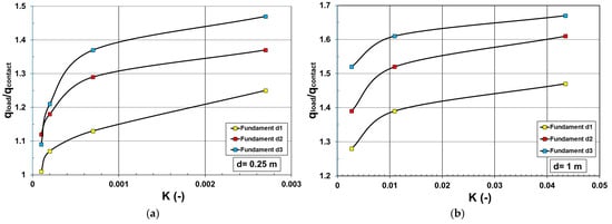
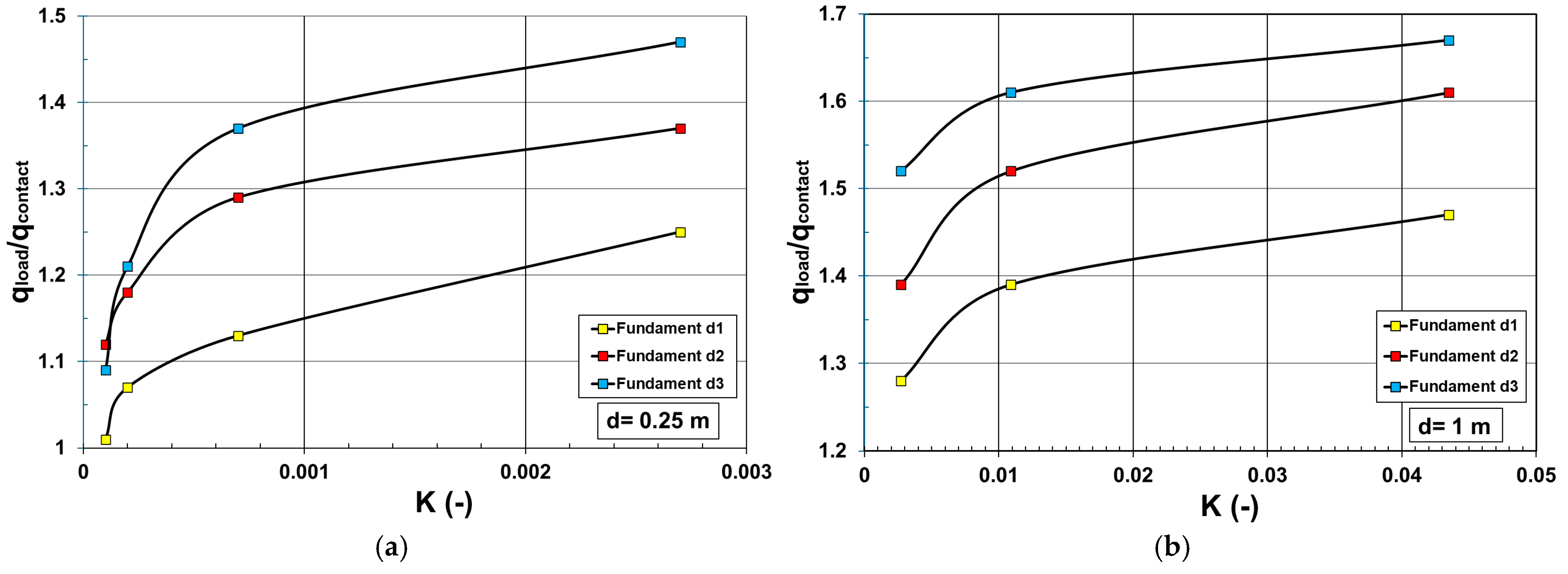
Figure 11.
Ratio of foundation load to contact pressure for foundations d1 to d3 depending on the relative stiffnesses of the soil–foundation systems: (a) foundation thickness = 0.25 m; (b) foundation thickness = 1 m.
The ratio of qload/qcontact is lower than 1.1 for the square-shaped foundations a1 to a3 and b1 to b3 (Figure 10) and lower than 1.15 for the rectangular-shaped foundation d1 with a single uniform load (Figure 11a) when the value of K is lower than 0.001. For foundations d2 and d3 in Figure 11a, which had varying cross-sections, the ratios of qload/qcontact are larger than 1.15 for K-values of between 0.0002 and 0.001. The relatively small contact areas of these foundations led to the relatively small settlements for the same uniform load.
For the rectangular-shaped foundations c2 and c3 with two uniformly distributed loads, the ratios of qload/qcontact are not provided. As demonstrated in Figure 5b,d, a relatively high difference between qload and qcontact arose in these foundations even for K = 0.0001. This resulted from the interaction between the foundation loads, so the deviations became higher with increasing difference between the foundation loads.
Finally, it can be stated that the value of K < 0.001 provided in Ref. [9] is satisfactory only for foundations with regular shapes and a single uniform load. In other cases, a value of K smaller than 0.001 is required to assume the systems as flexible.
3.2. Comparison of Subgrade Reaction Moduli Obtained from the Finite Element Analyses and Analytical Method Considering the Relative Stiffnesses of Soil–Foundation Systems
In the present section, the subgrade reaction moduli obtained from the FE analyses are compared to those from the analytical method by using four case studies, in which the effects of irregularities in foundation shape and in structural loads on the behavior of the soil–foundation systems are examined. Case studies 1 and 2 treat flexible soil–foundation systems, while rigid systems are studied in case studies 3 and 4 according to Refs. [8,9].
The analytical analyses were performed with the help of the software GGU-Settle Version 7.03 [29]. A uniformly distributed building load was first calculated using the ratio of building weight to foundation area. This load was then considered the contact pressure to determine the vertical stress distribution in soil based on the theory of Boussinesq [28]. Assuming that the soil–foundation system behaves infinitely rigidly or flexibly according to Refs. [8,9], the settlements were subsequently calculated based on the theory of elasticity [30]. Here, the thickness of the compressible soil layer was chosen considering the depth of settlement effect according to the German geotechnical standard. Finally, the distribution of the subgrade reaction modulus was determined by using the ratio of the contact pressure to the settlement.
3.2.1. Case Study 1
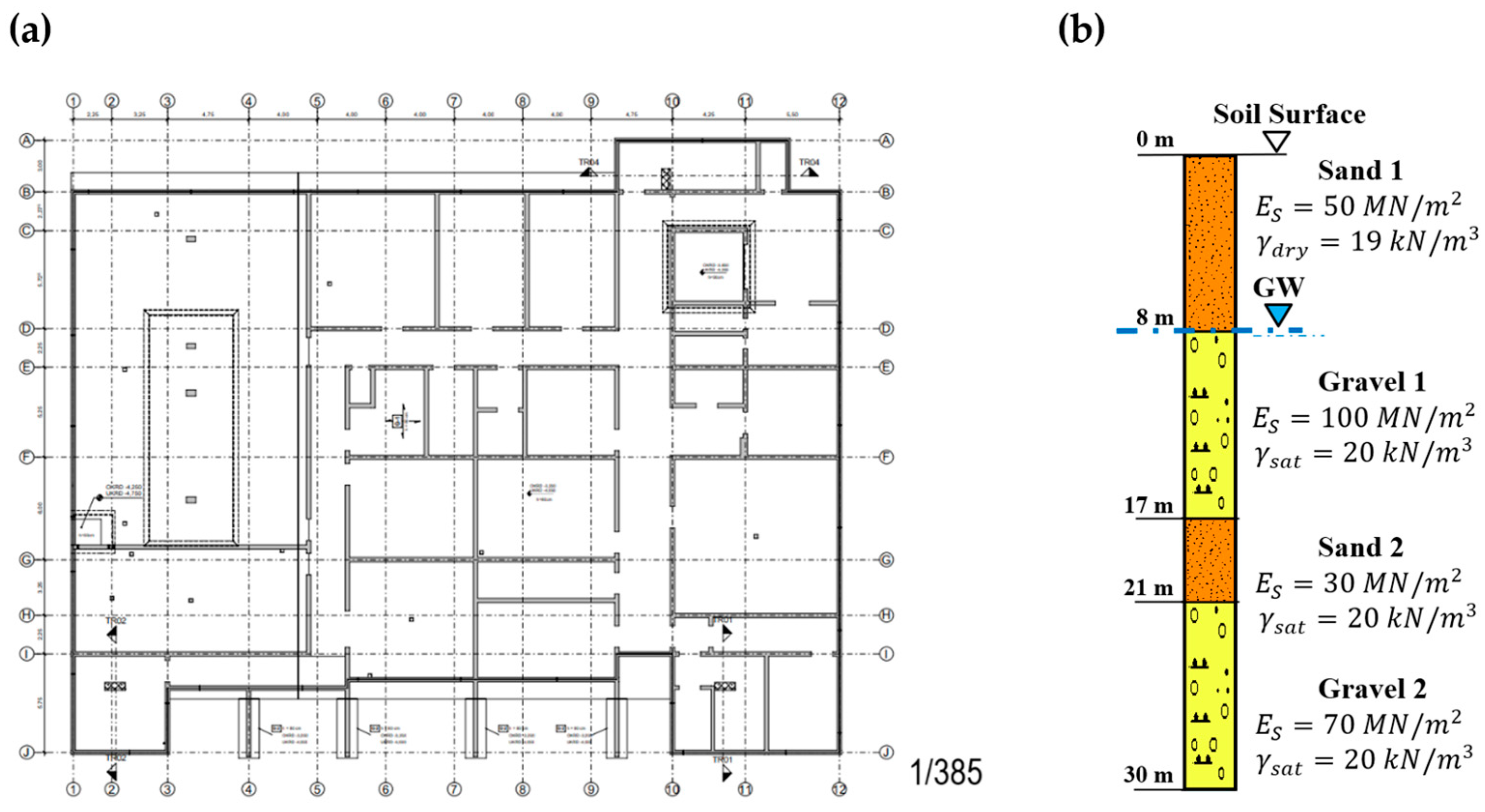
In the first case, the raft foundation of a multifamily residence was studied. The symmetrically shaped raft foundation illustrated in Figure 12a was constructed on the stratified soil provided in Figure 12b.
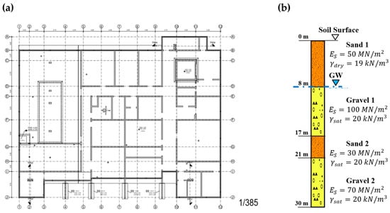
Figure 12.
Case study 1: (a) basement floor plan; (b) borehole log.
The foundation thickness of 0.75 m corresponded to its embedment depth. The base area of the raft foundation was about 1500 m2, and the building load, including the foundation weight, was 200 MN.
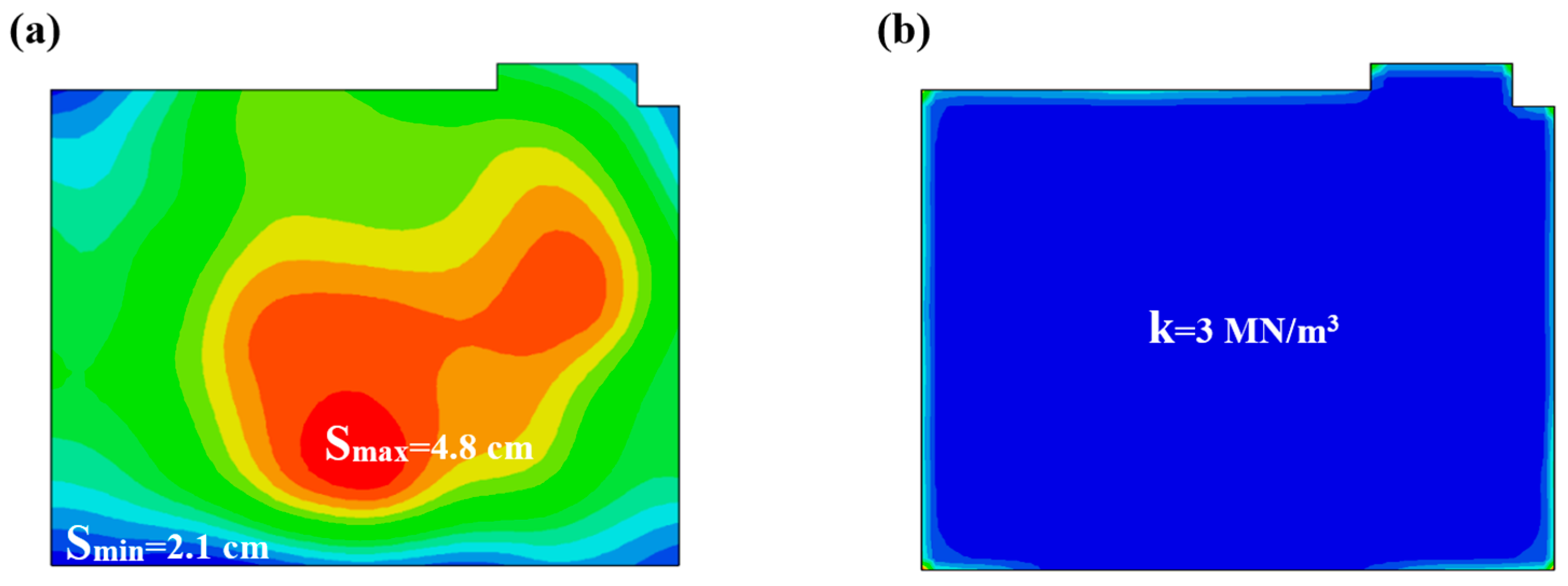
The finite element mesh consisted of isosceles right triangle elements with a congruent side length of 1 m. The FE analysis yielded a maximal settlement of 4.8 cm in the central area and a minimal settlement of 2.1 cm on the corner zones of the foundation (Figure 13a). The subgrade reaction modulus was determined as 3 MN/m3 except for the edge zones with a width of 2 m (Figure 13b). As a result of stress concentrations, the subgrade reaction modulus on the edge zones varied between 3 MN/m3 and 20 MN/m3.

Figure 13.
Results of the FE analysis for case study 1: (a) distribution of settlement; (b) distribution of subgrade reaction modulus.
For a fundament length of L = 45 m, a Young’s modulus of Ef = 31,000 MPa, and a constrained modulus of Es = 50 MPa, the relative stiffness of the soil–foundation system was calculated as K = 0.0002 using Equation (2). It corresponded to a flexible system according to Ref. [9], which can also be seen from the high difference of settlements in Figure 13a.
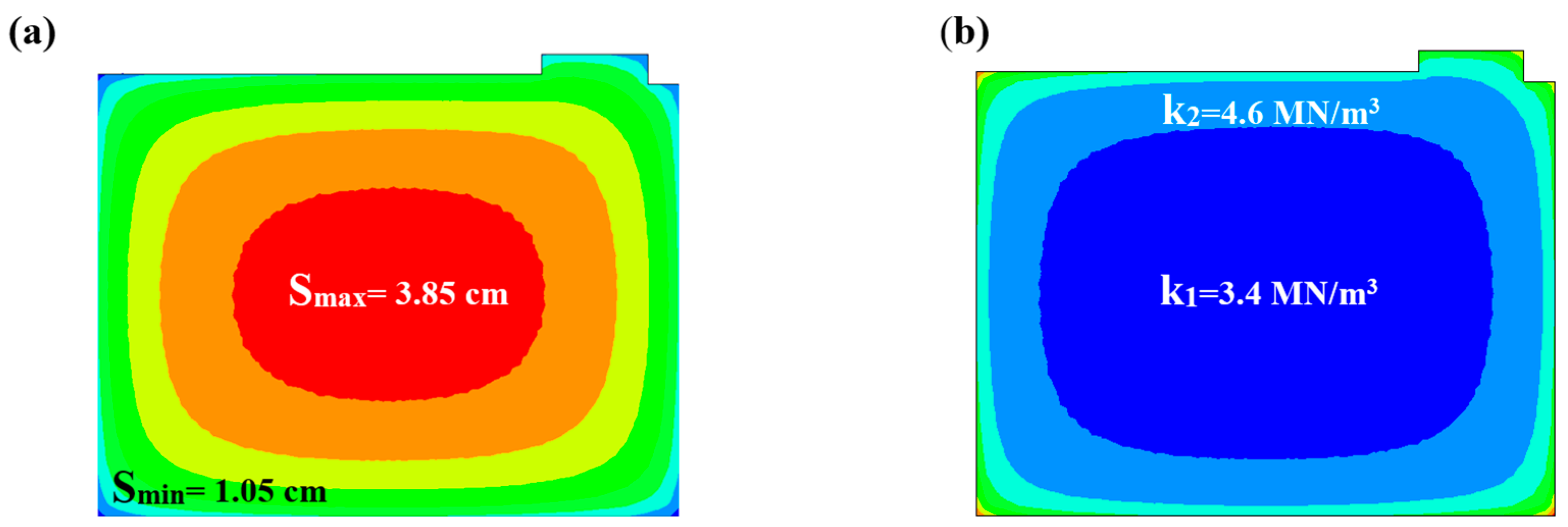
For the infinitely flexible system with a uniformly distributed contact pressure of q = 130 kN/m2, the distributions of settlements and subgrade reaction moduli obtained from the software GGU-Settle [29] are shown in Figure 14.

Figure 14.
Results of the analytical analysis for case study 1: (a) distribution of settlement with an increment of 0.4 cm; (b) distribution of subgrade reaction modulus with an increment of 1.2 MN/m3.
Following the settlements in Figure 14a, the modulus of subgrade reaction (k = q/S) increased step by step from the center to the edges of the foundation (Figure 14b). The analytical method yielded a subgrade reaction modulus of 3.4 MN/m3 in the central area of the foundation, which was relatively compatible with the value obtained from the FE analysis in Figure 13b. However, the analytical method yielded smaller settlement values than those of the FE analysis.
3.2.2. Case Study 2
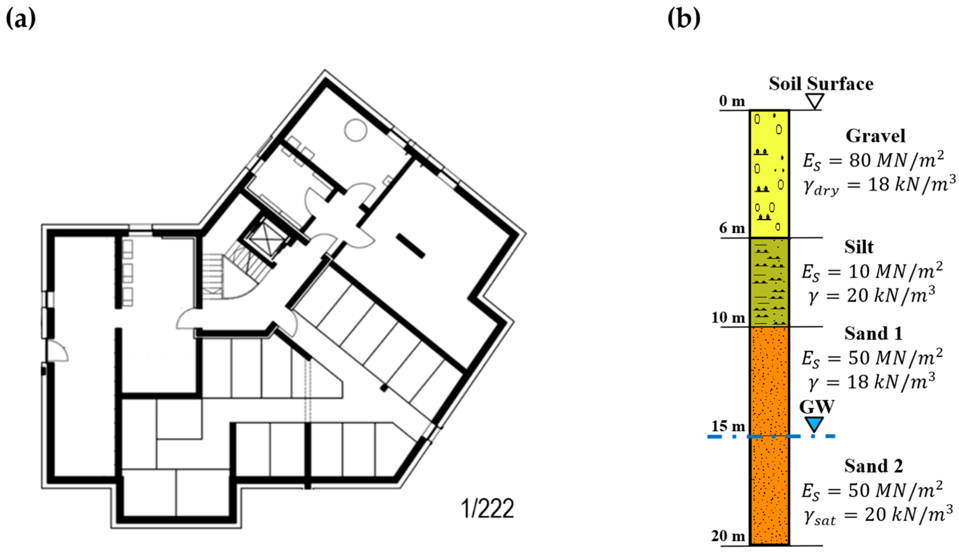
The raft foundation examined differs from case study 1 due to its asymmetrical shape (Figure 15a). The foundation of a multifamily residence was constructed on the stratified soil demonstrated in Figure 15b.
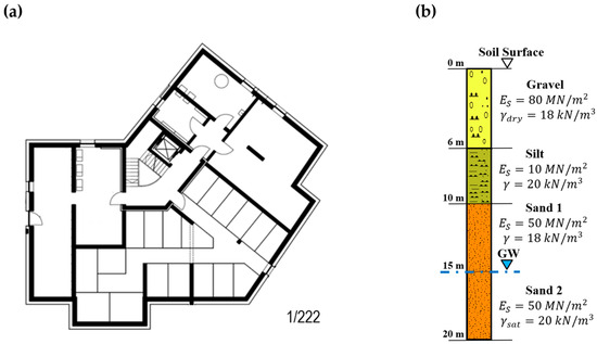
Figure 15.
Case study 2: (a) basement floor plan; (b) borehole log.
The foundation thickness was 0.5 m, corresponding to its embedment depth. The base area of the raft foundation was about 350 m2, and the building load, including the foundation weight, was 40 MN.
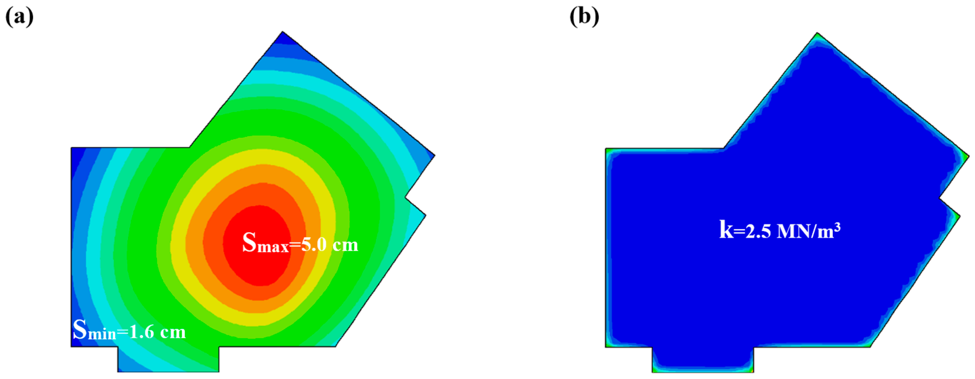
The finite element mesh consisted of isosceles right triangle elements with a congruent side length of 1 m. The FE analysis yielded a maximal settlement of 5 cm in the central area and a minimal settlement of 1.6 cm in the corner zones of the foundation (Figure 16a). The subgrade reaction modulus was determined as 2.5 MN/m3 in the central area of the foundation, while it varied between 2.5 MN/m3 and 20 MN/m3 in the edge zones with a width of 2 m (Figure 16b).

Figure 16.
Results of the FE analysis for case study 2: (a) distribution of settlement; (b) distribution of subgrade reaction modulus.
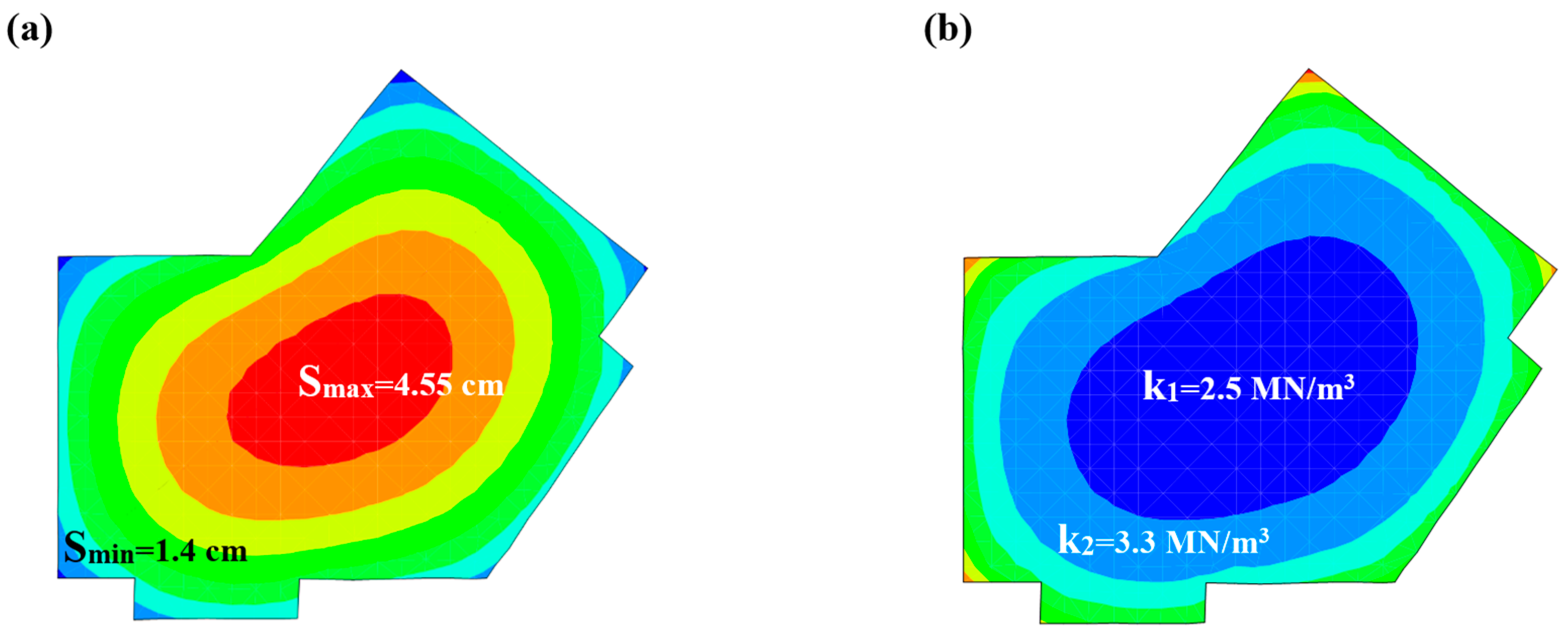
For the infinitely flexible system (K = 0.0003 for L = 24.5 m, Ef = 31,000 MPa, and Es = 80 MPa) with a uniformly distributed contact pressure of q = 115 kN/m2, the distributions of settlement and subgrade reaction modulus obtained from the analytical method are illustrated in Figure 17.

Figure 17.
Results of the analytical analysis for case study 2: (a) distribution of settlement with an increment of 0.45 cm; (b) distribution of subgrade reaction modulus with an increment of 0.8 MN/m3.
Compared to case study 1, the settlements obtained from the analytical method for case study 2 were relatively close to those in the FE analysis. The decisive factor was, in particular, the distribution of structural loads. Accordingly, both methods yielded the same value of the subgrade reaction modulus in the central area of the foundation. Similar behavior with respect to the subgrade reaction modulus was also observed for the foundations with K = 0.0001, 0.0002, and 0.0004 shown in Figure 3, so the ratio of kanalytical to kfem varied between 1.05 and 1.15 in the central area of the raft foundation.
3.2.3. Case Study 3
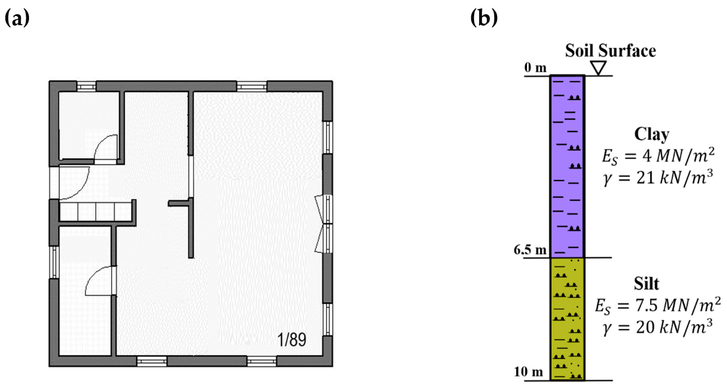
In this case, the raft foundation of a single-family home was studied. A symmetrically shaped raft foundation with a base area of 64 m2 was constructed on stratified soil (Figure 18). The foundation thickness of 0.5 m corresponded to its embedment depth, and the building load, including the foundation weight, was 3.3 MN.

Figure 18.
Case study 3: (a) basement floor plan; (b) borehole log.
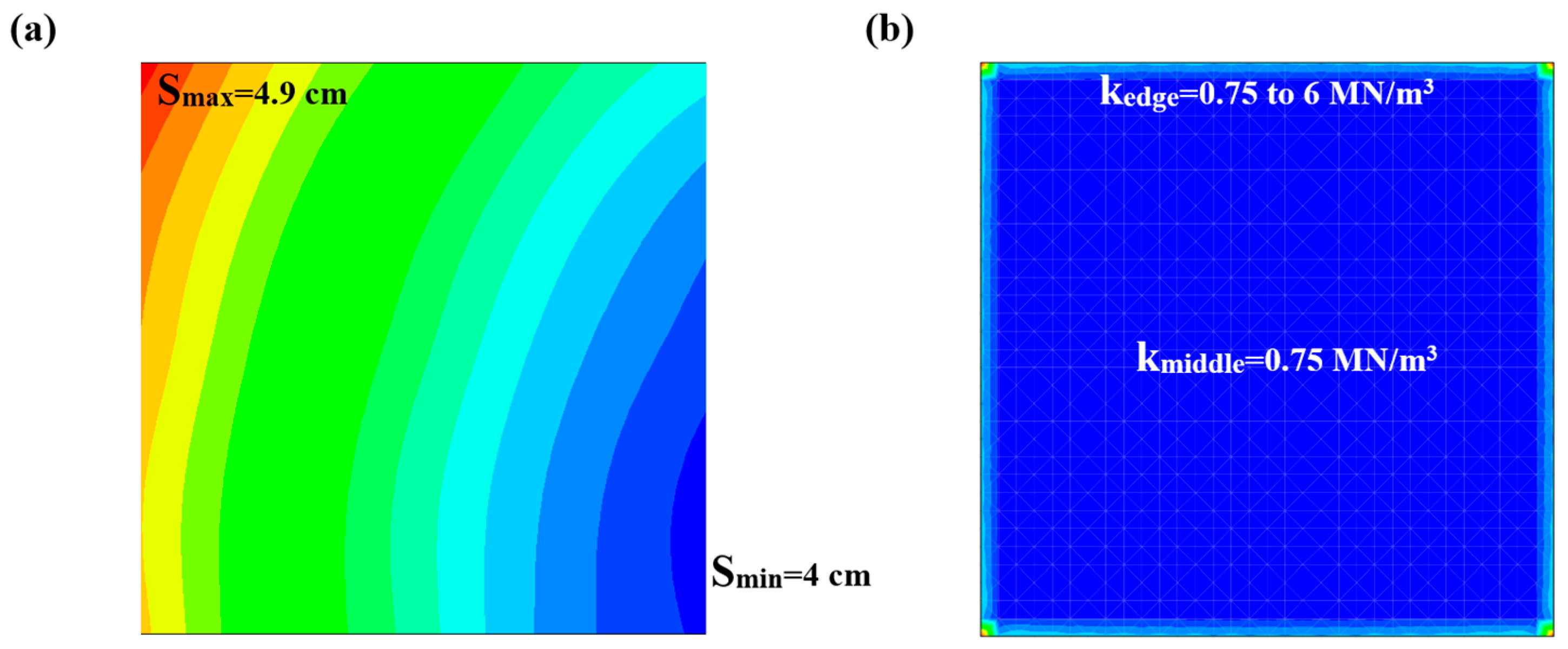
The finite element mesh consisted of isosceles right triangle elements with a congruent side length of 0.25 m. The maximal (4.9 cm) and minimal (4 cm) settlements arose in the corner zones of the foundation, as demonstrated in Figure 19a. The subgrade reaction modulus was determined as 0.75 MN/m3 in the central area of the foundation except for the edge zones with a width of 2 m, where its value varied between 0.75 MN/m3 and 6 MN/m3. The highest value of the subgrade reaction modulus (26 MN/m3) developed in the corner zones with an ignorable area size, where the highest structure loads acted (Figure 19b).

Figure 19.
Results of the FE analysis for case study 3: (a) distribution of settlement; (b) distribution of subgrade reaction modulus.
For the soil–foundation system with L = 8 m, Ef = 31,000 MPa, and Es = 4 MPa, the relative stiffness of the soil–foundation system was calculated as K = 0.1577 (infinitely rigid).
For a uniformly distributed contact pressure of q = 52 kN/m2, a uniform settlement of 3.65 cm and a correspondingly uniform subgrade reaction modulus of 1.42 MN/m3 were calculated using the software GGU-Settle based on the theory of elasticity [30].
3.2.4. Case Study 4
In the last case, the asymmetrically shaped raft foundation of a single-family home was examined (Figure 20a).
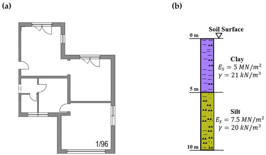
Figure 20.
Case study 4: (a) basement floor plan; (b) borehole log.
The raft foundation, with a base area of 48 m2 constructed on the soil shown in Figure 20b, had a thickness and an embedment depth of 0.5 m. The building load, including the foundation weight, was equal to 2.9 MN.
The finite element mesh consisted of isosceles right triangle elements with a congruent side length of 0.25 m. The maximal and minimal settlements obtained from the FE analysis were 3.7 and 3.1 cm, respectively (Figure 21a). The subgrade reaction modulus was determined as 1.05 MN/m3 in the central area of the foundation except for its edges with a width of 2 m, where its value varied between 1.05 MN/m3 and 8 MN/m3. As in case study 3, the highest contact pressure developed in the corner zones with an ignorable area size, which led to a relatively high subgrade reaction modulus of 34 MN/m3 (Figure 21b).
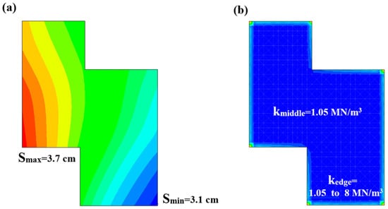
Figure 21.
Results of the FE analysis for case study 4: (a) distribution of settlement; (b) distribution of subgrade reaction modulus.
For the infinitely rigid foundation (K = 0.1860 for L = 7 m, Ef = 31,000 MPa, and Es = 5 MPa) with a uniformly distributed contact pressure of q = 60 kN/m2, the analytical method yielded a uniform settlement of about 3.3 cm and a correspondingly uniform subgrade reaction modulus of 1.8 MN/m3.
The analytical method yielded higher values of subgrade reaction moduli than those in FE analyses, so the ratios of kanalytical to kfem in the central area of the raft foundation were 1.9 and 1.7 for case studies 3 and 4, respectively. Similar behavior was also observed for the foundations with K ≥ 0.1739, shown in Figure 3, so the ratios of kanalytical to kfem varied between 1.5 and 1.9, which was relatively high compared to the ratios obtained from the flexible cases. This results from the fact that the contact pressure developing in the edge zones of a foundation increases with increasing relative stiffness of the system, which causes a corresponding decrease in the subgrade reaction modulus in the central area of the foundation obtained from FE analyses.
4. Conclusions
In the present work, an approximate procedure to estimate the subgrade reaction moduli of soil–raft foundation systems is studied based on the relative stiffnesses of soil–foundation systems suggested by DIN—Technical Report 130. The following results can be drawn from the analyses performed in the present study:
- (1)
- Concerning the estimation of the behavior of soil–foundation systems:
- -
- Assuming the soil–foundation systems are rigid, a value of K ≥ 0.174 is sufficient for foundations with symmetrical shapes and symmetrical distributions of uniformly distributed loads. In this case, the ratio of Smax/Smin is lower than 1.1.
- -
- Assuming the soil–foundation systems are flexible, a value of K ≤ 0.001 is satisfactory only for foundations with regular shapes and a single uniform load. In this case, the ratio of qload/qcontact is lower than 1.1 and 1.15 for the square-shaped and rectangular-shaped foundations, respectively.
- (2)
- Concerning the determination of subgrade reaction modulus:
- -
- For soil–foundation systems with K ≥ 0.174, the subgrade reaction moduli obtained from the conventional analytical method are about 1.5 to 2.0 times higher than those in the FE analyses considering the soil–foundation interaction;
- -
- For soil–foundation systems with K ≤ 0.0004, both the analytical and the FE methods yield similar values of subgrade reaction moduli. The ratio of kanalytical to kfem varies between 1.05 and 1.15.
The findings provided above enable geotechnical engineers to estimate the subgrade reaction modulus for raft foundations in the pre-design phase without the input of many structural loads, so the ratios of kanalytical to kfem in the central areas of the raft foundations of typical residential buildings vary between about 1.0 (flexible) and 2.0 (rigid), depending on the relative stiffnesses of soil–foundation systems calculated according to DIN—Technical Report 130.
The FE analyses indicated that the subgrade reaction modulus developing in the edge zones with a width of between 0.5 m and 2 m is higher than that in the central area of a foundation. The excessive increase in the subgrade reaction modulus in the edge zones can reach up to about 8 times of that in the central area of foundation.
Further studies are required for industrial buildings with locally high column loads.
Author Contributions
Conceptualization, S.K. and S.T.; methodology, S.K. and S.T.; software, S.K.; validation, S.K., formal analysis, S.T.; investigation, S.K. and S.T.; resources, S.K.; data curation, S.T.; writing—original draft preparation, S.T.; writing—review and editing, S.K. and S.T.; visualization, S.T.; supervision, S.K.; project administration, S.K. All authors have read and agreed to the published version of the manuscript.
Funding
The article processing charge was funded by Jade University of Applied Sciences in Germany.
Institutional Review Board Statement
Not applicable.
Informed Consent Statement
Not applicable.
Data Availability Statement
The data are contained within the article.
Conflicts of Interest
The authors declare no conflicts of interest.
References
- Winkler, E. Die Lehre von der Elastizität und Festigkeit; Dominicus: Prague, Czech Republic, 1867. [Google Scholar]
- Terzaghi, K. Evaluation of coefficient of subgrade reaction. Geotechnique 1955, 5, 297–326. [Google Scholar] [CrossRef]
- Daloglu, A.T.; Vallabhan, C.V.G. Values of k for slab on Winkler foundation. J. Geotech. Geoenvironmental Eng. 2000, 126, 463–471. [Google Scholar] [CrossRef]
- Alzoaby, H.; Saad, G.; Abou-Jaoude, G. Implementation of the discrete area method and its impact on the steel reinforcement of large mat foundations. Innov. Infrastruct. Solut. 2025, 10, 1–22. [Google Scholar] [CrossRef]
- Tabsh, S.W.; El-Emam, M. Influence of foundation rigidity on the structural response of mat foundation. Adv. Civ. Eng. 2021, 2021, 5586787. [Google Scholar] [CrossRef]
- Khosravifardshirazi, A.; Johari, A.; Javadi, A.A.; Khanjanpour, M.H.; Khosravifardshirazi, B.; Akrami, M. Role of Subgrade Reaction Modulus in Soil-Foundation-Structure Interaction in Concrete Buildings. Buildings 2022, 12, 540. [Google Scholar] [CrossRef]
- ACI, 336.2R-88; Suggested Analysis and Design Procedures for Combined Footings and Mats. ACI Committee: Farmington Hills, MI, USA, 2002.
- DIN-Fachbericht, 130. In Wechselwirkung Baugrund/Bauwerk Flachgründungen; Deutsches Institut für Normung e.V., Beuth-Verlag: Berlin, Deutschland, 2003.
- Bergmeister, K.; Wörner, J.-H. Beton-Kalender 2006: Schwerpunkt: Turmbauwerke, Industriebauten; Ernst&Sohn: Berlin, Germany, 2006. [Google Scholar]
- Brown, P.T. Numerical Analyses of Uniformly Loaded Circular Rafts on Deep Elastic Foundations. Geotechnique 1969, 19, 399–404. [Google Scholar] [CrossRef]
- El Gendy, M. An analysis for determination of foundation rigidity. In Proceedings of the 8th International Colloquium on Structural and Geotechnical Engineering, Cairo, Egypt, 15–17 December 1998. [Google Scholar]
- Lang, H.J.; Huder, J.; Amann, P.; Puzrin, A.M. Bodenmechanik und Grundbau (in German); Springer Verlag: Berlin, Germany, 2010. [Google Scholar]
- Biot, M.A. General theory of three-dimensional consolidation. J. Appl. Phys. 1941, 12, 155–164. [Google Scholar] [CrossRef]
- Vesic, A.B. Beams on elastic subgrade and the Winkler’s hypothesis. In Proceedings of the 5th International Conference on Soil Mechanics and Foundation Engineering, Paris, France, 17–22 July 1961. [Google Scholar]
- Bowles, J.E. Foundation Analysis and Design, 5th ed.; McGraw-Hill: New York, NY, USA, 1996. [Google Scholar]
- Poulos, H. Rational assessment of modulus of subgrade reaction. Geotech. Eng. J. SEAGS AGSSEA 2018, 49, 1–7. [Google Scholar] [CrossRef]
- Lee, J.; Jeong, S.; Lee, J.K. 3D analytical method for mat foundations considering coupled soil springs. Geomech. Eng. 2015, 8, 845–857. [Google Scholar] [CrossRef]
- Jeong, S.; Park, J.; Hong, M.; Lee, J. Variability of subgrade reaction modulus on flexible mat foundation. Geomech. Eng. 2017, 13, 757–774. [Google Scholar] [CrossRef]
- Loukidis, D.; Tamiolakis, G.P. Spatial distribution of Winkler spring stiffness for rectangular mat foundation analysis. Eng. Struct. 2017, 153, 443–459. [Google Scholar] [CrossRef]
- Son, M.; Jung, H.S.; Yoon, H.H.; Sung, D.; Kim, J.S. Numerical Study on Scale Effect of Repetitive Plate-Loading Test. Appl. Sci. 2019, 9, 4442. [Google Scholar] [CrossRef]
- Roy, S.S.; Deb, K. Modulus of subgrade reaction of unreinforced and georid-reinforced granular fill over soft clay. Int. J. Geomech. 2021, 21, 04021156. [Google Scholar] [CrossRef]
- Hamza, O.; Kourdey, A.; Hussain, Y.; Mawas, A. Subgrade reaction for closely spaced raft and isolated foundations on sand: Case study. Proc. Inst. Civ. Eng.-Geotech. Eng. 2024, 177, 135–146. [Google Scholar] [CrossRef]
- Rahgooy, K.; Bahmanpour, A.; Derakhshandi, M.; Bagherzadeh-Khalkhali, A. Distribution of elastoplastic modulus of subgrade reaction for analysis of raft foundations. Geomech. Eng. 2022, 28, 89–105. [Google Scholar] [CrossRef]
- Dehghanbanadaki, A.; Rashid, A.S.F.; Ahmad, K.; Yunus, N.Z.M.; Said, K.N.M. A computational estimation model for the subgrade reaction modulus of soil improved with DCM columns. Geomech. Eng. 2022, 28, 385–396. [Google Scholar] [CrossRef]
- Chang, D.-W.; Lu, C.-W.; Tu, Y.-J.; Cheng, S.-H. Settlements and Subgrade Reactions of Surface Raft Foundations Subjected to Vertically Uniform Load. Appl. Sci. 2022, 12, 5484. [Google Scholar] [CrossRef]
- Li, W.; Tao, Q.; Gu, R.; Li, C.; Dai, G.; Gong, W. Plate Size Effects in Gravelly Soil Based on In Situ Plate Load Tests and Finite Element Analysis. Appl. Sci. 2025, 15, 760. [Google Scholar] [CrossRef]
- Buß, J. GGU-Slab User Manual, version 12.04; Civilserve GmbH: Steinfeld, Germany, 2023. [Google Scholar]
- Boussinesq, J. Application des Potentiels à L’étude de L’équilibre et du Mouvement des Solides Élastiques; Gauthier-Villars: Paris, France, 1883. [Google Scholar]
- Buß, J. GGU-Settle User Manual, version 7.00; Civilserve GmbH: Steinfeld, Germany, 2023. [Google Scholar]
- DIN 4019:2015-05; Baugrund-Setzungsberechnungen. Deutsches Institut für Normung e.V., Beuth-Verlag: Berlin, Deutschland, 2015.


Disclaimer/Publisher’s Note: The statements, opinions and data contained in all publications are solely those of the individual author(s) and contributor(s) and not of MDPI and/or the editor(s). MDPI and/or the editor(s) disclaim responsibility for any injury to people or property resulting from any ideas, methods, instructions or products referred to in the content. |
© 2025 by the authors. Licensee MDPI, Basel, Switzerland. This article is an open access article distributed under the terms and conditions of the Creative Commons Attribution (CC BY) license (https://creativecommons.org/licenses/by/4.0/).