Tensor Product Alternatives for Nonlinear Field-Oriented Control of Induction Machines

Abstract

The paper presents a nonlinear field-oriented control technique based on the tensor product representation of the nonlinear induction machine model and the solvability of linear matrix inequalities. The nonlinear model has 32 quasi linear parameter-varying equivalent variants, and it is shown that only half of the models result in feasible controller. Two control goals are realized: torque control and speed control. The controller is a nonlinear state feedback controller completed by integral action. A new block diagram is investigated for speed control. The controller gains are designed by the solution of linear matrix inequalities to solve the Lyapunov inequality to obtain a stable and fast response and constraints on the control signal. The presented methods are verified and compared by simulations.

1. Introduction

Induction machines with a squirrel-cage rotor type have a simple and robust structure due to the lack of a commutator and brushes. In addition, these machines do not contain permanent magnets, resulting in a relatively low price and increased reliability since the demagnetization problem does not occur. These features make induction machines the most common in industrial drives [1], and also an attractive solution for automotive electric propulsion systems [2,3,4]. However, the performance of induction machine drives depends significantly on the control method used.

The earliest control approaches for induction machines are the so-called scalar control methods. By using them, the frequency and magnitude of the sinusoidal excitation voltages or currents can be adjusted. This allows the steady-state speed or torque to be controlled while keeping flux at the desired level. Since scalar control methods are based on steady-state equations of the machine, the control algorithms are simple and require low computational effort. In addition, an adequate steady-state characteristic can be achieved by using them. However, the scalar control has no effect on transients, so only weak or moderate dynamics are provided. Nevertheless, scalar control is widely used in low-cost and low-performance industrial applications such as pumps, compressors and fans [5,6].

Unlike scalar control, vector control techniques affect not only the frequency and magnitude of stator voltages or currents but also the direction of the space vectors since vector control methods are based on the transient description of the machine. As a result, much better dynamics can be achieved than with scalar control. The first vector control method is the well-known field-oriented control (FOC) introduced in [7,8]. The FOC principle is the indirect control of flux and torque through current controls, similar to the control of a separately excited DC machine. To separate the flux- and torque-producing componentsof the stator current vector, the coordinate system of the magnetic field is used for FOC. Originally, the rotor flux vector was used for field orientation, and it is still the most widespread. As alternatives to rotor flux orientation, stator flux [9] or air gap flux [10] reference frames can also be applied. However, these are rarely used in practical applications. Note that these traditional FOCs use linear control design, although induction machine models are nonlinear in nature. To compensate for the effects of nonlinearity, an additional decoupling algorithm is required, and the control performance depends on how accurately this algorithm works [11,12]. In contrast to scalar control, FOC provides better dynamics and very good properties at both low and high speeds [13]. It is also particularly important that the torque ripple is low over the entire speed range. The main drawbacks of FOC are its relatively high computational burden due to the coordinate transformations and its sensitivity to parameter mismatches as discussed in [1].

The second group of vector control includes the direct torque control (DTC) methods, which were introduced parallel to each other in [14,15]. The basic principles used in [14,15] are very similar, but the stator flux vector follows a circular trajectory in [14]; it is the so-called classical DTC, while direct self control (DSC) in [15] operates with a hexagonal stator flux vector trajectory. Both DTC methods are based on the effect of the possible switching states of the inverter on the behavior of the machine. Instead of using inner current control loops, DTCs directly control the stator flux and torque. To determine flux and torque feedback signals without direct measurement, estimators are applied in general. The main advantage of the conventional DTC and DSC methods is the extremely fast transient operation. In addition, these techniques do not require the information of the rotor angular velocity for torque control. In other words, the traditional DTCs are inherently rotary senorless methods, unlike FOC. Nevertheless, both FOC and DTC require angular velocity feedback for speed control. To replace the rotary sensors, fundamental frequency model-based estimators [16,17,18,19] and signal injection-based estimators [20,21,22] are also widely used. Due to the absence of coordinate transformation, pulse width modulation and inner current control loops, the conventional DTCs have a very simple structure and lower computational time than the FOC as presented in [23]. Furthermore, DTCs are less sensitive to parameter variations than FOC techniques. However, the original DTC methods are mostly not applicable in practice due to the extremely high current and torque ripples. To reduce current and torque ripples, several improvements have been developed for DTC, which are reviewed in [24,25]. But solving this problem increases the complexity of the control algorithm as discussed in [12].

In commercial drives, scalar control, FOC and improved DTC methods are the most popular due to their simplicity and easy tuning. However, more sophisticated control methods can be found in the literature. Since the difficulty of control design for induction machines is caused by the nonlinear description, nonlinear control theory offers attractive solutions. Among these, feedback linearization control (FLC) is used for induction machine drives in [26,27,28,29,30]. By using FLC, nonlinear transformation can be defined to represent the nonlinear induction machine model by independent linear subsystems. For these linear subsystems, advanced state feedback controllers, such as optimal or robust controllers, can be easily synthesized. It is important to highlight a theoretical similarity between FOC and FLC, namely that both control strategies use transformations to achieve a favorable mathematical description for control design. However, induction machine models in different coordinate systems can also be used for FLC. For example, Refs. [26,27,28] use stationary reference frame models, while rotor flux-oriented models are applied in [29,30]. The most significant disadvantages of FLC are the complex design procedure and the relative high computational burden.

A further promising approach in control design for nonlinear systems is the tensor product (TP) transformation [31,32,33,34]. TP model transformation is a modern framework to numerically approximate the linear time invariant (LTI), linear parameter varying (LPV) and quasi LPV (qLPV) representations of state-space models. The framework can replace the complicated derivations of the closed formulae of the state-space models with straightforward and numerically appealing solutions. Furthermore, it should be irrelevant how the state-space model is given (e.g., a set of closed formulae and a black box model). All in all, the nonlinear model is represented by the parameter-varying combination of LTI models; moreover, the TP model transformation was introduced as the higher-order singular value decomposition (HOSVD) of LPV models.

The TP model representation belongs to the class of polytopic models. The polytopic model-based state-space control design has three key steps:

• Defining the state-space model;
• Finding the optimal polytopic model (TP model in this paper);
• Deriving the controller.

The crucial point is that the model structure of steps 1 and 2 has a key role in determining the effectiveness of the controller design in step 3. The system matrix elements influence the controller design process in a strong sense. The convex hull defined by the polytopic structure in step 2 also directly influences the design. The system matrix elements can be obtained in a systematic way to check all the possible model representations. Controller design is usually carried out by the appropriate linear matrix inequalities (LMIs) based on the Lyapunov stability condition and constraint on the control input and on the control value [35].

Papers [36,37,38] deal with the fuzzy-state feedback controller design of induction machine with optimal performance. The Takagi–Sugeno fuzzy model is employed to approximate the nonlinear machine model in the FOC representation. A fuzzy controller is designed to stabilize the machine, and minimum disturbance attenuation is guaranteed via the ${\mathcal{H}}_{\infty }$-controller design. The LMI method is used to find controller gains.

Paper [39] presents a FOC-based technique; however, a nonlinear controller is derived using TP model transformation methodology. The classical FOC method and TP modeling are merged to control permanent magnet synchronous motors. Speed control is designed by the TP model approach, but the d-component of the current is controlled by a PI-controller. Simulation results show better performance in terms of overshoot, speed and disturbance rejection when compared to the results of conventional cascade PI + PI control solution.

The paper [40] proposes the design of an induction machine controller based on the TP method, and the sum of square (SOS) method is used to set up performance criterion constraints in polynomial form instead of the LMIs. Reference signal tracking is realized efficiently.

The induction machine nonlinear TP-based controller is complemented by an integral action and observer in [41,42]. The designed controller ensures stable and accurate operation over the full operating range of the machine, taking into account the wide range of temperature values, and possible variations in inductances, which are outside the range of the parameters under consideration.

In summary, the main challenge in the control of induction machines is caused by the nonlinear mathematical description. To solve the problem of nonlinear models, different solutions are used in FOC, DTC, FLC and the above discussed TP-based control methods. Among them, the FOC is the most widespread, which uses simple linear controllers and compensates for nonlinear effects by decoupling. Therefore, the performance depends on the decoupling algorithm. The conventional DTCs use nonlinear hysteresis controllers, which result in high current and torque ripples. Although FLC avoids decoupling, as well as high current and torque ripples, it requires complex formulae to be defined. In contrast, the TP model transformation-based control is numerical and easy to algorithmize. Therefore, high performance and easy to implement control methods can be achieved by combining FOC and TP transformation, similarly to [40,41,42]. However, the idea of [43] shows that a TP model has a huge number of alternatives. These variants can be readily derived by the TP model transformation that can variate the number of fuzzy rules, the number of antecedent and consequent sets, and, further, the shape of the antecedent fuzzy sets. The goal of this paper is to analyze the behavior of model alternatives from the controller design viewpoint. The FOC-based state-space model is used in the frame of TP modeling and LMI-based control synthesis for torque control and speed control.

Although this paper focuses on the control of induction machines, the proposed methodology can be applied in general to other problems of which the TP model representation can be used for control design.

2. Materials and Methods

2.1. Tensor Product Model Transformation

The most important results of the TP model transformation will be summarized shortly based on the papers [31,32,33,34].

Consider the linear parameter-varying state-space model

$$\begin{array}{cc}\hfill \dot{\mathbf{x}}\left(t\right)=& \mathbf{A}\left(\mathbf{p}\right(t\left)\right)\mathbf{x}\left(t\right)+\mathbf{B}\left(\mathbf{p}\right(t\left)\right)\mathbf{u}\left(t\right),\hfill \\ \hfill \mathbf{y}\left(t\right)=& \mathbf{C}\left(\mathbf{p}\right(t\left)\right)\mathbf{x}\left(t\right)+\mathbf{D}\left(\mathbf{p}\right(t\left)\right)\mathbf{u}\left(t\right),\hfill \end{array}$$

(1)

where $\mathbf{x}=\mathbf{x}\left(t\right)\in {\mathbb{R}}^m$, $\mathbf{u}=\mathbf{u}\left(t\right)\in {\mathbb{R}}^k$ and $\mathbf{y}=\mathbf{y}\left(t\right)\in {\mathbb{R}}^l$ are the state vector, the input vector, and the output vector with the dimension of m, k, and l, respectively. Matrices $\mathbf{A}$, $\mathbf{B}$, $\mathbf{C}$, and $\mathbf{D}$ depend on the parameter vector $\mathbf{p}=\mathbf{p}\left(t\right)\in \Omega$. The parameter vector consists of N parameters, depending on the model description, $\mathbf{p}={[p_1{p}_2\cdots p_N]}^{\mathrm{T}}$. The set $\Omega$ is a hyper space, i.e., $\Omega ={\omega }_1\times {\omega }_2\times \cdots \times {\omega }_N$, where ${\omega }_i$ is an interval of the according parameter $p_i$, i.e., ${\omega }_i=[{\omega }_i^{min},{\omega }_i^{max}]$. The applied hyper space $\Omega$ as well as the selected parameter vector $\mathbf{p}$ are discussed later in Section 2.2 and Section 2.4.

The system matrix is defined by

$$\mathbf{S}=\mathbf{S}\left(\mathbf{p}\right)=\left[\begin{array}{cc}\mathbf{A}\left(\mathbf{p}\right(t\left)\right)& \mathbf{B}\left(\mathbf{p}\right(t\left)\right)\\ \mathbf{C}\left(\mathbf{p}\right(t\left)\right)& \mathbf{D}\left(\mathbf{p}\right(t\left)\right)\end{array}\right]\in {\mathbb{R}}^{(m+l)\times (m+k)}.$$

(2)

The main idea of TP model transformation is to discretize the given model state-space representation over a hyper rectangular grid M in $\Omega$, then the tensor product structure of the model is obtained via executing higher-order singular value decomposition. By ignoring singular values, the TP model of reduced complexity and accuracy can be obtained.

The tensor product structure can be written as follows:

$$\mathbf{S}=\mathcal{S}{⊠}_{n=1}^N{\mathbf{w}}_n\left(p_n\right)=\sum _{i_1=1}^{I_1}\sum _{i_2=1}^{I_2}\cdots \sum _{i_N=1}^{I_N}\prod _{n=1}^N{w}_{n,i_n}\left(p_n\right)S_{i_1,i_2,\cdots i_N},$$

(3)

where $\mathcal{S}\in {\mathbb{R}}^{I_1\times I_2\times \cdots \times I_N\times (m+l)\times (m+k)}$ is the core tensor, the vector ${\mathbf{w}}_n$ contains the weighting functions $w_{n,i_n}\left(p_n\right)$, $I_n$ denotes the number of LTI systems in the nth dimension of the domain $\Omega$, and $S_{i_1,i_2,\cdots i_N}$ is a LTI system. The symbol ⊠ denotes multiple n-mode products of a tensor by a matrix.

The transformation steps and the corresponding controller design scheme are detailed below.

2.2. Induction Machine Model

The nonlinear ordinary differential equations of a set of nonlinear systems have the following general formula [44]:

$$\dot{\mathbf{x}}=\mathbf{f}\left(\mathbf{x}\right)+\mathbf{g}\left(\mathbf{x}\right)\mathbf{u},$$

(4)

where $\mathbf{x}$ is the state variable vector, the nonlinear mapping $\mathbf{f}\left(\mathbf{x}\right)$ has the special form of $\mathbf{f}\left(\mathbf{x}\right)=\mathbf{A}\left(\mathbf{x}\right)\mathbf{x}$, and $\mathbf{g}\left(\mathbf{x}\right)$ is constant, denoted by the matrix $\mathbf{B}$, i.e., systems with the differential equations $\dot{\mathbf{x}}=\mathbf{A}\left(\mathbf{x}\right)\mathbf{x}+\mathbf{B}\mathbf{u}$ are studied in this paper, meaning that the parameter vector $\mathbf{p}$ can be equal to the state vector $\mathbf{p}=\mathbf{x}$ or a part of the state vector—furthermore, a function of state vector elements. The system input is denoted by $\mathbf{u}$.

The nonlinear mapping and the constant matrix of an induction machine can be written in the rotor flux-oriented model as [45,46,47,48]

$$\mathbf{f}\left(\mathbf{x}\right)=\left[\begin{array}{c}-\frac{R_{\mathrm{s}}{L}_{\mathrm{r}}^2+R_{\mathrm{r}}{L}_{\mathrm{m}}^2}{\sigma L_{\mathrm{s}}{L}_{\mathrm{r}}^2}{i}_{\mathrm{sd}}+\frac{R_{\mathrm{r}}{L}_{\mathrm{m}}}{\sigma L_{\mathrm{s}}{L}_{\mathrm{r}}^2}{\psi }_{\mathrm{rd}}+p{\omega }_{\mathrm{m}}{i}_{\mathrm{sq}}+\frac{R_{\mathrm{r}}{L}_{\mathrm{m}}}{L_{\mathrm{r}}}\frac{i_{\mathrm{sq}}^2}{{\psi }_{\mathrm{rd}}}\\ -\frac{R_{\mathrm{s}}{L}_{\mathrm{r}}^2+R_{\mathrm{r}}{L}_{\mathrm{m}}^2}{\sigma L_{\mathrm{s}}{L}_{\mathrm{r}}^2}{i}_{\mathrm{sq}}-\frac{p{L}_{\mathrm{m}}}{\sigma L_{\mathrm{s}}{L}_{\mathrm{r}}}{\omega }_{\mathrm{m}}{\psi }_{\mathrm{rd}}-p{\omega }_{\mathrm{m}}{i}_{\mathrm{sd}}-\frac{R_{\mathrm{r}}{L}_{\mathrm{m}}}{L_{\mathrm{r}}}\frac{i_{\mathrm{sd}}{i}_{\mathrm{sq}}}{{\psi }_{\mathrm{rd}}}\\ \frac{R_{\mathrm{r}}{L}_{\mathrm{m}}}{L_{\mathrm{r}}}{i}_{\mathrm{sd}}-\frac{R_{\mathrm{r}}}{L_{\mathrm{r}}}{\psi }_{\mathrm{rd}}\\ \frac{3}{2}\frac{p}{J}\frac{L_{\mathrm{m}}}{L_{\mathrm{r}}}{i}_{\mathrm{sq}}{\psi }_{\mathrm{rd}}-\frac{D_{\mathrm{f}}}{J}{\omega }_{\mathrm{m}}-\frac{1}{J}{T}_{\mathrm{L}}\end{array}\right],$$

(5)

and

$$\mathbf{g}\left(\mathbf{x}\right)=\mathbf{B}=\left[\begin{array}{cc}\frac{1}{\sigma L_{\mathrm{s}}}& 0\\ 0& \frac{1}{\sigma L_{\mathrm{s}}}\\ 0& 0\\ 0& 0\end{array}\right].$$

(6)

The resistance and self-induction coefficient of the three windings of the stator and of the rotor are denoted by $R_{\mathrm{s}}$, $L_{\mathrm{s}}$, $R_{\mathrm{r}}$ and $L_{\mathrm{r}}$; furthermore, $L_{\mathrm{m}}$ is the mutual inductance between the stator and rotor coils, and $\sigma$ is a parameter depending on the the inductances $\sigma =1-\frac{L_{\mathrm{m}}^2}{L_{\mathrm{s}}{L}_{\mathrm{r}}}$. The pole pair number is denoted by p, and J and $D_{\mathrm{f}}$ are the moment of inertia and the viscous friction coefficient. The state variables are the d and q components of the stator current, denoted by $i_{\mathrm{sd}}$ and $i_{\mathrm{sq}}$, the d component is of the rotor flux ${\psi }_{\mathrm{rd}}$, and ${\omega }_{\mathrm{m}}$ is the mechanical speed of the rotor, i.e.,

$$\mathbf{x}={\left[\begin{array}{cccc}{i}_{\mathrm{sd}}& i_{\mathrm{sq}}& {\psi }_{\mathrm{rd}}& {\omega }_{\mathrm{m}}\end{array}\right]}^{\mathrm{T}}.$$

(7)

The load torque $T_{\mathrm{L}}$ is a disturbance model input. Finally, the motor torque is obtained by

$$T=\frac{3}{2}p\frac{L_{\mathrm{m}}}{L_{\mathrm{r}}}{i}_{\mathrm{sq}}{\psi }_{\mathrm{rd}}.$$

(8)

Dividing by ${\psi }_{\mathrm{rd}}$ is replaced by variable $p_5$, i.e., $p_5=1/{\psi }_{\mathrm{rd}}$ is a new model parameter (element of the parameter vector $\mathbf{p}$), which, by dividing by zero, can be handled.

Varying the state vector elements, the matrix $\mathbf{A}=\mathbf{A}\left(\mathbf{p}\right)$ of the model (5) can be rewritten as the following general form:

$$\begin{array}{cc}\hfill \mathbf{A}=& \left[\begin{array}{ccc}-\frac{R_{\mathrm{s}}{L}_{\mathrm{r}}^2+R_{\mathrm{r}}{L}_{\mathrm{m}}^2}{\sigma L_{\mathrm{s}}{L}_{\mathrm{r}}^2}& \frac{R_{\mathrm{r}}{L}_{\mathrm{m}}}{L_{\mathrm{r}}}{i}_{\mathrm{sq}}{p}_5+p{\omega }_{\mathrm{m}}A& \cdots \\ -p{\omega }_{\mathrm{m}}B-\frac{R_{\mathrm{r}}{L}_{\mathrm{m}}}{L_{\mathrm{r}}}{i}_{\mathrm{sq}}{p}_{5}C& -\frac{R_{\mathrm{s}}{L}_{\mathrm{r}}^2+R_{\mathrm{r}}{L}_{\mathrm{m}}^2}{\sigma L_{\mathrm{s}}{L}_{\mathrm{r}}^2}-\frac{R_{\mathrm{r}}{L}_{\mathrm{m}}}{L_{\mathrm{r}}}{i}_{\mathrm{sd}}{p}_5(1-C)& \cdots \\ \frac{R_{\mathrm{r}}{L}_{\mathrm{m}}}{L_{\mathrm{r}}}& 0& \cdots \\ 0& \frac{3}{2}\frac{p}{J}\frac{L_{\mathrm{m}}}{L_{\mathrm{r}}}{\psi }_{\mathrm{rd}}E& \cdots \end{array}\right.\hfill \\ \hfill & \left.\begin{array}{ccc}\cdots & \frac{R_{\mathrm{r}}{L}_{\mathrm{m}}}{\sigma L_{\mathrm{s}}{L}_{\mathrm{r}}^2}& p{i}_{\mathrm{sq}}(1-A)\\ \cdots & -\frac{p{L}_{\mathrm{m}}}{\sigma L_{\mathrm{s}}{L}_{\mathrm{r}}}{\omega }_{\mathrm{m}}D& -p{i}_{\mathrm{sd}}(1-B)-\frac{p{L}_{\mathrm{m}}}{\sigma L_{\mathrm{s}}{L}_{\mathrm{r}}}{\psi }_{\mathrm{rd}}(1-D)\\ \cdots & -\frac{R_{\mathrm{r}}}{L_{\mathrm{r}}}& 0\\ \cdots & \frac{3}{2}\frac{p}{J}\frac{L_{\mathrm{m}}}{L_{\mathrm{r}}}{i}_{\mathrm{sq}}(1-E)& -\frac{D_{\mathrm{f}}}{J}\end{array}\right].\hfill \end{array}$$

(9)

With the five new parameters A, B, C, D and E, all the possible 32 qLPV models can be analyzed from the viewpoint of modeling and controller design. The new parameters can be selected from the discrete set of $\{0,1\}$.

Table 1. The 32 qLPV models of the studied induction machine.

#	E	D	C	B	A	${\mathit{i}}_{\mathbf{sd}}$	${\mathit{i}}_{\mathbf{sq}}$	${\mathit{\psi }}_{\mathbf{rd}}$	${\mathit{\omega }}_{\mathbf{m}}$	${\mathit{p}}_5$	R
0	0	0	0	0	0	x a	x	x	-	x	16
1	0	0	0	0	1	x	x	x	x	x	32
2	0	0	0	1	0	x	x	x	x	x	32
3	0	0	0	1	1	x	x	x	x	x	32
4	0	0	1	0	0	x	x	x	-	x	16
5	0	0	1	0	1	x	x	x	x	x	32
6	0	0	1	1	0	-	x	x	x	x	16
7	0	0	1	1	1	-	x	x	x	x	16
8	0	1	0	0	0	x	x	-	x	x	16
9	0	1	0	0	1	x	x	-	x	x	16
10	0	1	0	1	0	x	x	-	x	x	16
11	0	1	0	1	1	x	x	-	x	x	16
12	0	1	1	0	0	x	x	-	x	x	16
13	0	1	1	0	1	x	x	-	x	x	16
14	0	1	1	1	0	-	x	-	x	x	8
15	0	1	1	1	1	-	x	-	x	x	8
16	1	0	0	0	0	x	x	x	-	x	16
17	1	0	0	0	1	x	-	x	x	x	16
18	1	0	0	1	0	x	x	x	x	x	32
19	1	0	0	1	1	x	-	x	x	x	16
20	1	0	1	0	0	x	x	x	-	x	16
21	1	0	1	0	1	x	x	x	x	x	32
22	1	0	1	1	0	-	x	x	x	x	16
23	1	0	1	1	1	-	x	x	x	x	16
24	1	1	0	0	0	x	x	x	x	x	32
25	1	1	0	0	1	x	-	x	x	x	16
26	1	1	0	1	0	x	x	x	x	x	32
27	1	1	0	1	1	x	-	x	x	x	16
28	1	1	1	0	0	x	x	x	x	x	32
29	1	1	1	0	1	x	x	x	x	x	32
30	1	1	1	1	0	-	x	x	x	x	16
31	1	1	1	1	1	-	x	x	x	x	16

^a Notation x means that the variable appears in the system model.

depicts all the 32 qLPV models, where the dependency of the matrix $\mathbf{A}$ on the parameters can also be seen (for example, $\mathbf{p}={\left[i_{\mathrm{sd}}{i}_{\mathrm{sq}}{\psi }_{\mathrm{rd}}{p}_5\right]}^{\mathrm{T}}$ for model #1, or $\mathbf{p}={\left[i_{\mathrm{sq}}{\omega }_{\mathrm{m}}{p}_5\right]}^{\mathrm{T}}$ for model #15, i.e., the parameter vector contains state variables, functions of state variables, or other relevant parameters).

The following output matrices ${\mathbf{C}}_i$ ($i=0,1,2,3$) are chosen in the analysis to define the output vector $\mathbf{y}={\mathbf{C}}_i\mathbf{x}={\left[y_1{y}_2\right]}^{\mathrm{T}}$. The index i represents the different output vectors as follows.

The classical field-oriented control scheme can be given by

$${\mathbf{C}}_0=\left[\begin{array}{cccc}1& 0& 0& 0\\ 0& 1& 0& 0\end{array}\right],$$

(10)

i.e., $y_1=i_{\mathrm{sd}}$ and $y_2=i_{\mathrm{sq}}$. The reference currents along the d and q axes can be obtained from the reference flux and torque as it will be presented later.

The reference flux and torque can be directly controlled by the output matrices

$${\mathbf{C}}_1=\left[\begin{array}{cccc}0& 0& 1& 0\\ 0& \frac{3}{2}p\frac{L_{\mathrm{m}}}{L_{\mathrm{r}}}{\psi }_{\mathrm{rd}}& 0& 0\end{array}\right],$$

(11)

and

$${\mathbf{C}}_2=\left[\begin{array}{cccc}0& 0& 1& 0\\ 0& 0& \frac{3}{2}p\frac{L_{\mathrm{m}}}{L_{\mathrm{r}}}{i}_{\mathrm{sq}}& 0\end{array}\right],$$

(12)

i.e., $y_1={\psi }_{\mathrm{rd}}$ and $y_2=T=\frac{3}{2}p\frac{L_{\mathrm{m}}}{L_{\mathrm{r}}}{i}_{\mathrm{sq}}{\psi }_{\mathrm{rd}}$.

The reference flux and speed can be directly controlled by the output matrix of

$${\mathbf{C}}_3=\left[\begin{array}{cccc}0& 0& 1& 0\\ 0& 0& 0& 1\end{array}\right],$$

(13)

i.e., $y_1={\psi }_{\mathrm{rd}}$ and $y_2={\omega }_{\mathrm{m}}$.

The matrix $\mathbf{D}$ is zero.

All in all, $32\times 4=128$ models are set up and analyzed.

2.3. Model Parameters

The asynchronous motor model nominal parameters are chosen as follows, where their physical meaning is also given [49]:

• Number of pole pairs, $p=2$;
• Stator resistance, $R_{\mathrm{s}}=4.7\Omega$;
• Rotor resistance, $R_{\mathrm{r}}=5.2\Omega$;
• Stator self inductance, $L_{\mathrm{s}}=0.1788\mathrm{H}$;
• Rotor self inductance, $L_{\mathrm{r}}=0.1790\mathrm{H}$;
• Mutual inductance, $L_{\mathrm{m}}=0.1690\mathrm{H}$;
• Moment of inertia, $J=0.00108\mathrm{kg}{\mathrm{m}}^2$;
• Viscous friction coefficient, $D_{\mathrm{f}}=0.00475\mathrm{Nms}$.

and $\sigma =1-\frac{L_{\mathrm{m}}^2}{L_{\mathrm{s}}{L}_{\mathrm{r}}}$ is the leakage coefficient.

2.4. Model Discretization Parameters

The following parameters are set when the model matrices are discretized in the grid M. Here, the problem region $\Omega$ as well as the region limits are listed:

• The problem region for models 0, 4, 16, and 20 is

  $$\Omega =[i_{\mathrm{sd}}^{\min },i_{\mathrm{sd}}^{\max }]\times [i_{\mathrm{sq}}^{\min },i_{\mathrm{sq}}^{\max }]\times [{\psi }_{\mathrm{rd}}^{\min },{\psi }_{\mathrm{rd}}^{\max }]\times [p_5^{\min },p_5^{\max }];$$
• The problem region for models 8, 9, 10, 11, 12, and 13 is

  $$\Omega =[i_{\mathrm{sd}}^{\min },i_{\mathrm{sd}}^{\max }]\times [i_{\mathrm{sq}}^{\min },i_{\mathrm{sq}}^{\max }]\times [{\omega }^{\min },{\omega }^{\max }]\times [p_5^{\min },p_5^{\max }];$$
• The problem region for models 1, 2, 3, 5, 17, 18, 19, 21, 24, 25, 26, 27, 28, and 29 is

  $$\Omega =[i_{\mathrm{sd}}^{\min },i_{\mathrm{sd}}^{\max }]\times [i_{\mathrm{sq}}^{\min },i_{\mathrm{sq}}^{\max }]\times [{\psi }_{\mathrm{rd}}^{\min },{\psi }_{\mathrm{rd}}^{\max }]\times [{\omega }^{\min },{\omega }^{\max }]\times [p_5^{\min },p_5^{\max }];$$
• The problem region for models 6, 7, 22, 23, 30, and 31 is

  $$\Omega =[i_{\mathrm{sq}}^{\min },i_{\mathrm{sq}}^{\max }]\times [{\psi }_{\mathrm{rd}}^{\min },{\psi }_{\mathrm{rd}}^{\max }]\times [{\omega }^{\min },{\omega }^{\max }]\times [p_5^{\min },p_5^{\max }];$$
• The problem region for models 14 and 15 is

  $$\Omega =[i_{\mathrm{sq}}^{\min },i_{\mathrm{sq}}^{\max }]\times [{\omega }^{\min },{\omega }^{\max }]\times [p_5^{\min },p_5^{\max }].$$

The limit values are set to

• $i_{\mathrm{sd}}^{\min }=-10\mathrm{A}$, $i_{\mathrm{sd}}^{\max }=10\mathrm{A}$;
• $i_{\mathrm{sq}}^{\min }=-10\mathrm{A}$, $i_{\mathrm{sq}}^{\max }=10\mathrm{A}$;
• ${\psi }_{\mathrm{rd}}^{\min }=0.1\mathrm{mVs}$, ${\psi }_{\mathrm{rd}}^{\max }=2\mathrm{Vs}$;
• ${\omega }^{\min }=-200\mathrm{rad}/\mathrm{s}$, ${\omega }^{\max }=200\mathrm{rad}/\mathrm{s}$;
• $p_5^{\min }=01/\mathrm{Vs}$, $p_5^{\max }=10\mathrm{k}/\mathrm{Vs}$.

The limit values are relevant for the studied motor from the paper [49]. All the intervals are divided into 20 segments.

2.5. Tensor Product-Based Controller Design

The mentioned control system is a nonlinear state feedback controller completed by the integral action to eliminate the steady-state error of the step response and to attenuate disturbance and noise effects [41,42,50].

2.5.1. Reference and Disturbance Data

The flux and torque reference values are set as follows:

$${\psi }_{\mathrm{rd}}^{\mathrm{ref}}=0.2\mathrm{Vs},T^{\mathrm{ref}}=0.4\mathrm{Nm}.$$

From these reference values, the reference currents $i_{\mathrm{sd}}$ and $i_{\mathrm{sq}}$ can be calculated as

$$i_{\mathrm{sd}}^{\mathrm{ref}}=\frac{{\psi }_{\mathrm{rd}}^{\mathrm{ref}}}{L_{\mathrm{m}}}=1.1834\mathrm{A},i_{\mathrm{sq}}^{\mathrm{ref}}=\frac{2}{3}\frac{L_{\mathrm{r}}}{p{L}_{\mathrm{m}}}\frac{T^{\mathrm{ref}}}{{\psi }_{\mathrm{rd}}^{\mathrm{ref}}}=0.7061\mathrm{A},$$

i.e., the reference current components contains the nominal value of the inductances $L_{\mathrm{m}}$ and $L_{\mathrm{r}}$.

In the case of speed control,

$${\omega }_{\mathrm{ref}}=\frac{T_{\mathrm{ref}}}{D_{\mathrm{f}}}=84.2105\frac{\mathrm{rad}}{\mathrm{s}}$$

is adopted.

The load torque is defined as

$$T_{\mathrm{L}}=\left\{\begin{array}{ccc}0,& \mathrm{if}& t<T_1;\\ 0.4,& \mathrm{if}& T_1\leqq t<T_2;\\ -0.4,& \mathrm{if}& t\geqq T_2.\end{array}\right.$$

In the case of torque control, $T_1=1.5\mathrm{s}$, and $T_2=3\mathrm{s}$; furthermore, in the case of speed control, $T_1=6\mathrm{s}$, $T_2=9\mathrm{s}$.

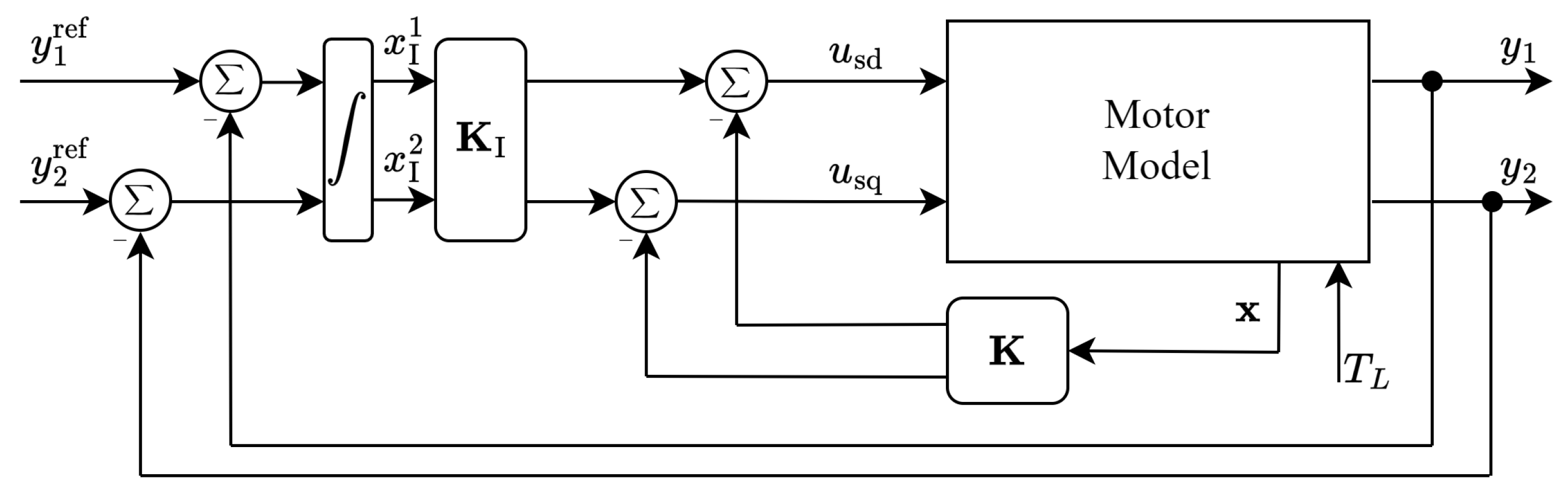
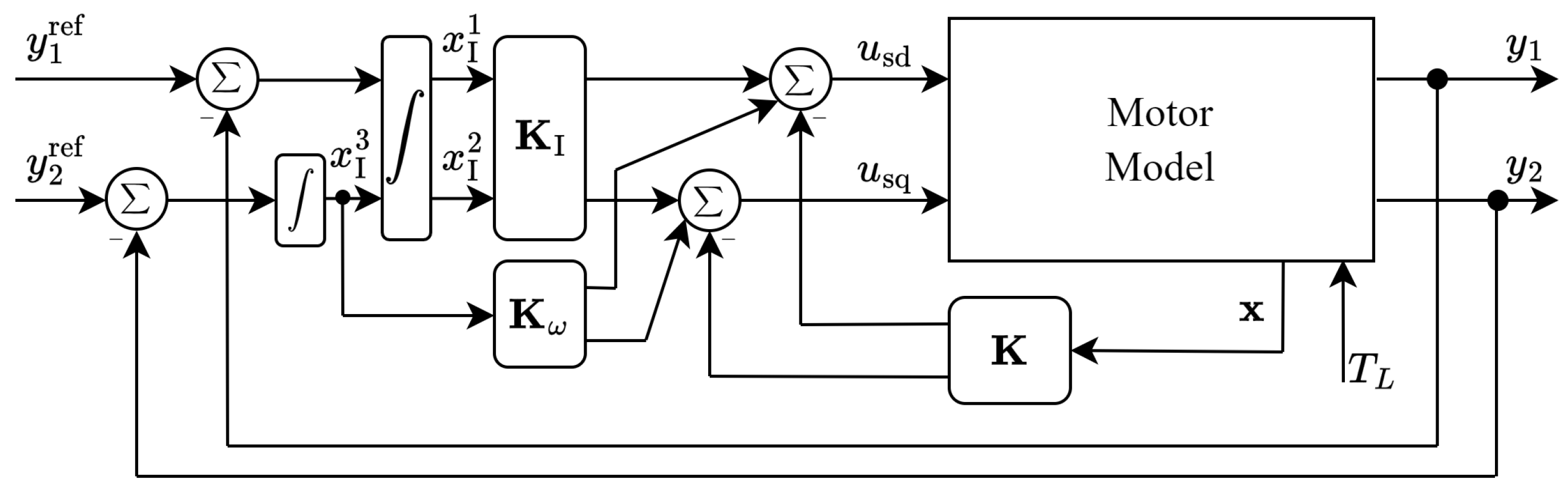
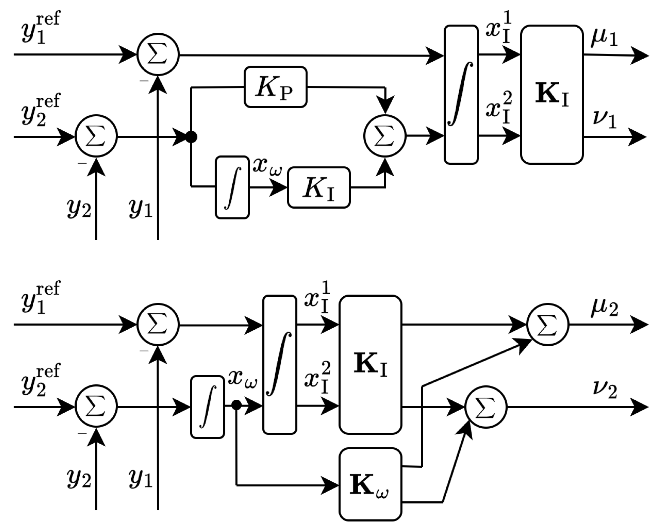
2.5.2. Controller Block Diagrams

Two control goals are realized in the frame of tensor product modeling: torque control and speed control.

• The torque control scheme

The torque control scheme is depicted in Figure 1. The plant is the induction machine model with two inputs and two outputs: $u_{\mathrm{sd}}$ and $u_{\mathrm{sq}}$ are the d and q components of the stator voltage in the dq reference frame; $y_1$ and $y_2$ can be defined by the output matrix of ${\mathbf{C}}_0$, ${\mathbf{C}}_1$ or ${\mathbf{C}}_2$, as well as the reference components $y_1^{\mathrm{ref}}$ and $y_2^{\mathrm{ref}}$. The state $\mathbf{x}$ is applied in the state feedback part of the controller, denoted by $\mathbf{K}=\mathbf{K}\left(\mathbf{x}\right)$. The error components between the reference signals and the outputs are plugged into the feedforward block of the controller, denoted by the matrix ${\mathbf{K}}_{\mathrm{I}}={\mathbf{K}}_{\mathrm{I}}\left(\mathbf{x}\right)$. The feedforward block contains an integrator for the two channels independently. The motor is affect by the load torque $T_{\mathrm{L}}$.

The plant input in Figure 1 can be written as follows:

$$\mathbf{u}=\left[\begin{array}{c}{u}_{\mathrm{sd}}\\ u_{\mathrm{sq}}\end{array}\right]=-\mathbf{K}\mathbf{x}+{\mathbf{K}}_{\mathrm{I}}{\int }_{-\infty }^t\left(\left[\begin{array}{c}{y}_1^{\mathrm{ref}}-y_1\\ y_2^{\mathrm{ref}}-y_2\end{array}\right]\right)\mathrm{d}\tau ,$$

(14)

where the dimensions of the matrices $\mathbf{K}$ and ${\mathbf{K}}_{\mathrm{I}}$ are $2\times 4$ and $2\times 2$, respectively.

The errors are defined as

$${\dot{x}}_{\mathrm{I}}^1=y_1^{\mathrm{ref}}-y_1,\mathrm{and}{\dot{x}}_{\mathrm{I}}^2=y_2^{\mathrm{ref}}-y_2,$$

with which the following augmented system can be defined for controller design using the notation ${\mathbf{x}}_{\mathrm{I}}={\left[x_{\mathrm{I}}^1{x}_{\mathrm{I}}^2\right]}^{\mathrm{T}}$:

$$\begin{array}{c}\hfill \left[\begin{array}{c}\dot{\mathbf{x}}\\ {\dot{\mathbf{x}}}_{\mathrm{I}}\end{array}\right]=\left[\begin{array}{cc}{\mathbf{A}}^{4\times 4}& {\mathbf{0}}^{4\times 2}\\ {\mathbf{C}}_i^{2\times 4}& {\mathbf{0}}^{2\times 2}\end{array}\right]\left[\begin{array}{c}\mathbf{x}\\ {\mathbf{x}}_{\mathrm{I}}\end{array}\right]+\left[\begin{array}{c}{\mathbf{B}}^{4\times 2}\\ {\mathbf{0}}^{2\times 2}\end{array}\right]\mathbf{u},\end{array}$$

(15)

$$\mathbf{u}=-\left[\begin{array}{cc}\mathbf{K}& {\mathbf{K}}_{\mathrm{I}}\end{array}\right]\left[\begin{array}{c}\mathbf{x}\\ {\mathbf{x}}_{\mathrm{I}}\end{array}\right],$$

(16)

and $i=0,1,2$. The matrices can be designed by the solution of an LMI problem.

• The speed control scheme

The control algorithm mentioned in Figure 1 is extended to the control rotational speed. The block diagram of the speed control is shown in Figure 2, where a new state variable $x_{\mathrm{I}}^3$ and a new feedforward block ${\mathbf{K}}_{\omega }$ are introduced (this is a column vector with two rows); moreover, $y_1={\psi }_{\mathrm{rd}}$, and $y_2={\omega }_{\mathrm{m}}$ are chosen, i.e., the flux and rotor speed are the reference signal components.

The error $y_2^{\mathrm{ref}}-y_2$ is processed by a PI controller block in the original field-oriented control scheme to generate a reference torque ($y_2^{\mathrm{ref}}={\omega }_{\mathrm{m}}^{\mathrm{ref}}$ and $y_2={\omega }_{\mathrm{m}}$) [7,8,45,46,47,48]. This cascade PI controller must be reformulated to have the state feedback and integrator feedforward formula.

The details of the PI controller reformulation based on Figure 3 are as follows.

First, the original field-oriented control scheme extended for speed control contains a PI controller whose input is the error signal $y_2^{\mathrm{ref}}-y_2$. This PI block is copied to the second channel of Figure 3, resulting in the upper scheme. Let us denote the error signal by

$${\dot{x}}_{\omega }=y_2^{\mathrm{ref}}-y_2.$$

(17)

The PI output signal is the input of the next integrator, i.e.,

$${\dot{x}}_{\mathrm{I}}^2=K_{\mathrm{P}}{\dot{x}}_{\omega }+K_{\mathrm{I}}{x}_{\omega },$$

(18)

in other words

$$x_{\mathrm{I}}^2=K_{\mathrm{P}}{x}_{\omega }+K_{\mathrm{I}}{\int }_{-\infty }^t{x}_{\omega }\mathrm{d}\tau .$$

(19)

With these, the integrator block output followed by the matrix ${\mathbf{K}}_{\mathrm{I}}$ is

$$\begin{array}{cc}\hfill {\mu }_1=& K_{11}{x}_{\mathrm{I}}^1+K_{12}\left(K_{\mathrm{P}}{x}_{\omega }+K_{\mathrm{I}}{\int }_{-\infty }^t{x}_{\omega }\mathrm{d}\tau \right),\hfill \\ \hfill {\nu }_1=& K_{21}{x}_{\mathrm{I}}^1+K_{22}\left(K_{\mathrm{P}}{x}_{\omega }+K_{\mathrm{I}}{\int }_{-\infty }^t{x}_{\omega }\mathrm{d}\tau \right).\hfill \end{array}$$

(20)

Second, the integrator output signal on the second channel in the bottom of Figure 3 is

$${\dot{x}}_{\mathrm{I}}^2=x_{\omega },$$

(21)

i.e.,

$$x_{\mathrm{I}}^2={\int }_{-\infty }^t{x}_{\omega }\mathrm{d}\tau .$$

(22)

The P and I part constants of the original field-oriented control scheme can be moved to the vector ${\mathbf{K}}_{\omega }$. With these, the integrator block output followed by the matrix ${\mathbf{K}}_{\mathrm{I}}$ and the vector ${\mathbf{K}}_{\omega }$ is

$$\begin{array}{cc}\hfill {\mu }_2=& K_{11}{x}_{\mathrm{I}}^1+K_{12}{x}_{\mathrm{I}}^2+K_{\omega ,1}{x}_{\omega }=K_{11}{x}_{\mathrm{I}}^1+K_{12}{\int }_{-\infty }^t{x}_{\omega }\mathrm{d}\tau +K_{\omega ,1}{x}_{\omega },\hfill \\ \hfill {\nu }_2=& K_{21}{x}_{\mathrm{I}}^1+K_{22}{x}_{\mathrm{I}}^2+K_{\omega ,2}{x}_{\omega }=K_{21}{x}_{\mathrm{I}}^1+K_{22}{\int }_{-\infty }^t{x}_{\omega }\mathrm{d}\tau +K_{\omega ,2}{x}_{\omega }.\hfill \end{array}$$

(23)

By the appropriate choice of the integrator parameters, ${\mu }_2={\mu }_1$ and ${\nu }_2={\nu }_1$ can be realized, i.e., the mentioned block diagram can be applied to control motor speed via state feedback control.

The control signals of Figure 2 are given as:

$$\left[\begin{array}{c}{u}_{\mathrm{sd}}\\ u_{\mathrm{sq}}\end{array}\right]=-\mathbf{K}\mathbf{x}+{\mathbf{K}}_{\mathrm{I}}{\int }_{-\infty }^t\left(\left[\begin{array}{c}{y}_1^{\mathrm{ref}}-y_1\\ {\int }_{-\infty }^t(y_2^{\mathrm{ref}}-y_2)\mathrm{d}\xi \end{array}\right]\right)\mathrm{d}\tau +{\mathbf{K}}_{\omega }{\int }_{-\infty }^t(y_2^{\mathrm{ref}}-y_2)\mathrm{d}\tau .$$

(24)

In this case, the augmented system can be written as

$$\begin{array}{c}\hfill \left[\begin{array}{c}\dot{\mathbf{x}}\\ {\dot{\mathbf{x}}}_{\mathrm{I}}\\ {\dot{x}}_{\omega }\end{array}\right]=\left[\begin{array}{cc}{\mathbf{A}}^{4\times 4}& {\mathbf{0}}^{4\times 3}\\ \left[\begin{array}{cccc}0& 0& 1& 0\\ 0& 0& 0& 0\\ 0& 0& 0& 1\end{array}\right]& \left[\begin{array}{ccc}0& 0& 0\\ 0& 0& 1\\ 0& 0& 0\end{array}\right]\end{array}\right]\left[\begin{array}{c}\mathbf{x}\\ {\mathbf{x}}_{\mathrm{I}}\\ x_{\omega }\end{array}\right]+\left[\begin{array}{c}{\mathbf{B}}^{4\times 2}\\ {\mathbf{0}}^{3\times 2}\end{array}\right]\mathbf{u},\end{array}$$

(25)

$$\mathbf{u}=-\left[\begin{array}{ccc}\mathbf{K}& {\mathbf{K}}_{\mathrm{I}}& {\mathbf{K}}_{\omega }\end{array}\right]\left[\begin{array}{c}\mathbf{x}\\ {\mathbf{x}}_{\mathrm{I}}\\ x_{\omega }\end{array}\right],$$

(26)

whose representation can be used to design a nonlinear controller which contains the PI-term for torque generation in a nonlinear form which is applicable in the TP-based framework.

2.5.3. Controller Design

Controller synthesis is performed via the following steps:

• Define the motor parameters, references, and other data such as the load torque signal (see Section 2.3 and Section 2.5.1).
• Define parameter vector $\mathbf{p}$ according to the analyzed TP model alternative (i.e., select parameters A, B, C, D, and E). It is based on Table 1.
• Define the parameter space $\Omega$, and its discretization (see Section 2.4).
• Set up system matrix $\mathbf{A}$, input and output matrices $\mathbf{B}$ and ${\mathbf{C}}_i$ ($i=0,1,2,3$) based on Table 1 and on the equations in Section 2.2.
• Set up the matrices according to the block diagram in Figure 1 for torque control or in Figure 2 for rotor speed control, i.e., according to (15) or (25). For example, set up the matrix

  $$\left[\begin{array}{ccc}{\mathbf{A}}^{4\times 4}& {\mathbf{0}}^{4\times 2}& {\mathbf{B}}^{4\times 2}\\ {\mathbf{C}}_i^{2\times 4}& {\mathbf{0}}^{2\times 2}& {\mathbf{0}}^{2\times 2}\end{array}\right],$$

  or

  $$\left[\begin{array}{ccc}{\mathbf{A}}^{4\times 4}& {\mathbf{0}}^{4\times 3}& {\mathbf{B}}^{4\times 2}\\ \left[\begin{array}{cccc}0& 0& 1& 0\\ 0& 0& 0& 0\\ 0& 0& 0& 1\end{array}\right]& \left[\begin{array}{ccc}0& 0& 0\\ 0& 0& 1\\ 0& 0& 0\end{array}\right]& {\mathbf{0}}^{3\times 2}\end{array}\right];$$
• Run higher-order singular value decomposition using the above mentioned matrix;
• Set up weighting functions and vertex systems according to the approximation by

  $$\begin{array}{cc}\hfill \dot{\mathbf{x}}=& \sum _{n=1}^R{w}_n\left(\mathbf{p}\right)\left({\mathbf{A}}_n\mathbf{x}+{\mathbf{B}}_n\mathbf{u}\right),\hfill \end{array}$$

  (27)

  where R is the number vertex systems (see Table 1 for the applied linear systems of the different TP model alternatives), ${\mathbf{A}}_n$ and ${\mathbf{B}}_n$ are the linear system matrices in the vertices, and $w_n\left(\mathbf{p}\right)$ is the weighting function. In this study, only CNO (Close-To-Normality) and IRNO (Inverse-Relaxed-Normality) functions are studied; however, other weighting functions can be selected, such as SNNN (Sum-Normalized and Non Negativeness) [31,32,33,34];
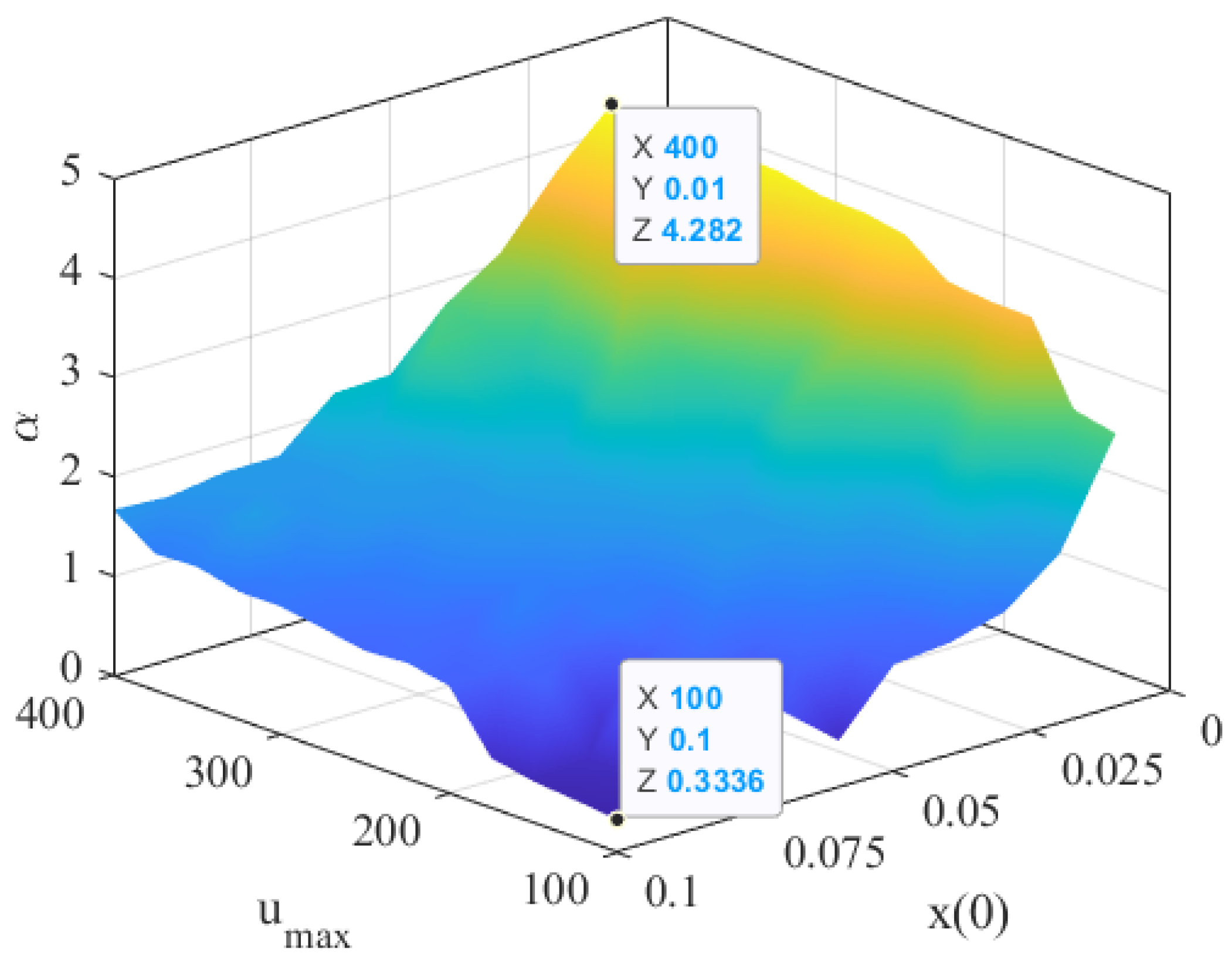
• The control goal is to speed up the system response. In this case, the so-called decay rate control can be applied, i.e., to solve the following generalized eigenvalue minimization problem with linear matrix inequalities [35]:

  $$\begin{array}{cc}\hfill & \mathrm{maximize}\alpha ,\mathrm{subject}\mathrm{to}\hfill \\ \hfill & \mathbf{X}\succ \mathbf{0},\hfill \\ \hfill & -\mathbf{X}{\mathbf{A}}_n^{\mathrm{T}}-{\mathbf{A}}_n\mathbf{X}+{\mathbf{M}}_n^{\mathrm{T}}{\mathbf{B}}_n^{\mathrm{T}}+{\mathbf{B}}_n{\mathbf{M}}_n-2\alpha \mathbf{X}\succ \mathbf{0},\hfill \\ \hfill & -\mathbf{X}{\mathbf{A}}_n^{\mathrm{T}}-{\mathbf{A}}_n\mathbf{X}-\mathbf{X}{\mathbf{A}}_m^{\mathrm{T}}-{\mathbf{A}}_m\mathbf{X}+{\mathbf{M}}_m^{\mathrm{T}}{\mathbf{B}}_n^{\mathrm{T}}+{\mathbf{B}}_n{\mathbf{M}}_m+{\mathbf{M}}_n^{\mathrm{T}}{\mathbf{B}}_m^{\mathrm{T}}+{\mathbf{B}}_m{\mathbf{M}}_n-4\alpha \mathbf{X}⪰\mathbf{0},\hfill \end{array}$$

  (28)

  where $n=1,\cdots ,R$, and $m=n+1,\cdots ,R$.
  The control goal is augmented by the control value constraint. Assuming that the state initial value is bounded, i.e., $\left|\right|\mathbf{x}\left(0\right)\left|\right|\le \varphi$ ($\varphi$ is predefined), the constraint ${\left|\right|\mathbf{u}\left(t\right)\left|\right|}_2\le u_{\max }$ can be enforced at all times $t\ge 0$ if the following linear matrix inequalities hold:

  $$\begin{array}{cc}\hfill & {\varphi }^2\mathbf{I}⪯\mathbf{X},\hfill \\ \hfill & \left[\begin{array}{cc}\mathbf{X}& {\mathbf{M}}_n^{\mathrm{T}}\\ {\mathbf{M}}_n& u_{\max }^2\mathbf{I}\end{array}\right]⪰\mathbf{0},n=1,\cdots ,R.\hfill \end{array}$$

  (29)
  The maximum value of the parameter $\alpha$ can be found by the simple bisection method as follows:

  –

  Set the interval $[a,\cdots ,b]$ where $\alpha$ is assumed;

  –

  While $|b-a|>\epsilon$ do the following iteration ($\epsilon$ is a small positive limit, $\epsilon ={10}^{-5}$ is used):

  *

  $x=\frac{a+b}{2}$;

  *

  Solve the above mentioned LMI with $\alpha =x$;

  *

  If LMI is feasible, then $a=x$; otherwise, $b=x$.

  –

  $\alpha =x$.

• Vertex gain matrices are obtained by

  $${\mathbf{K}}_n={\mathbf{M}}_n{\mathbf{X}}^{-1},n=1,\cdots ,R,$$

  (30)

  from which the feedback and feedforward gains in (16) or in (26) can be calculated:

  $$\mathbf{u}=-\sum _{n=1}^R{w}_n\left(\mathbf{p}\right){\mathbf{K}}_n\left[\begin{array}{c}\mathbf{x}\\ {\mathbf{x}}_{\mathrm{I}}\end{array}\right],\mathrm{or}\mathbf{u}=-\sum _{n=1}^R{w}_n\left(\mathbf{p}\right){\mathbf{K}}_n\left[\begin{array}{c}\mathbf{x}\\ {\mathbf{x}}_{\mathrm{I}}\\ x_{\omega }\end{array}\right],$$

  (31)

  if torque control or speed control is running.
• Check the closed-loop control system. Feasibility and applicability checks are performed, and the results are shown in the next section.

3. Results

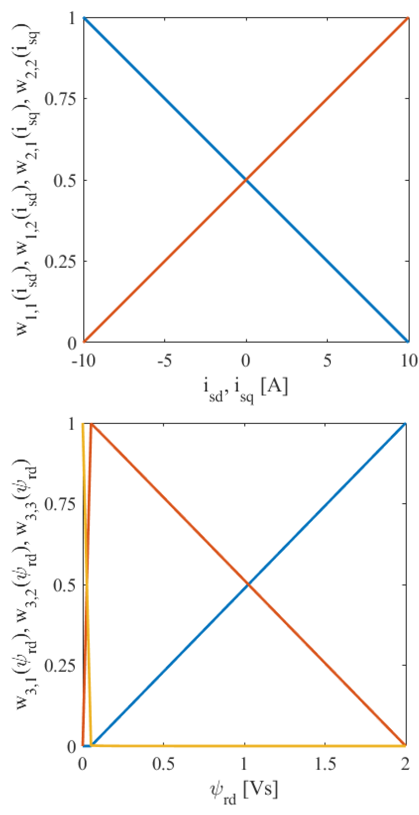
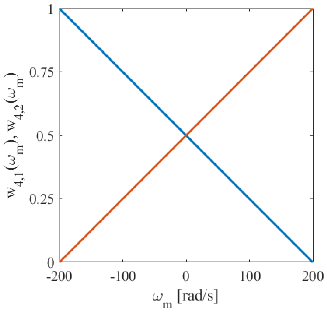
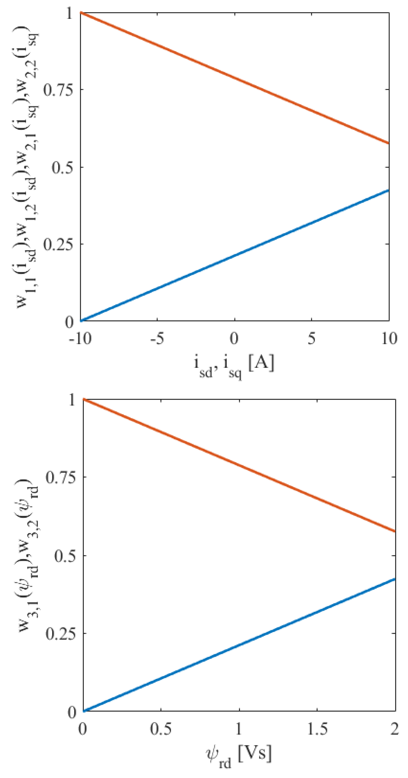
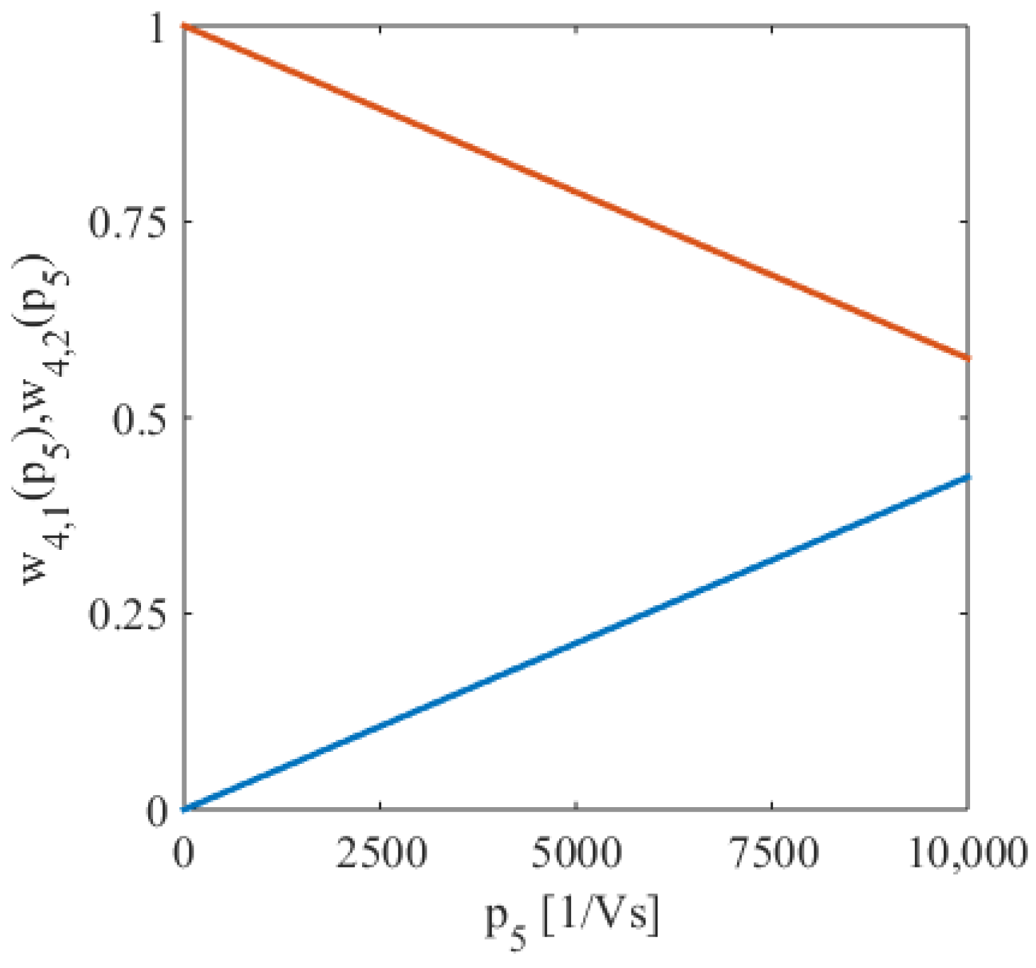
3.1. The Weighting Functions

Figure 4 shows the CNO-type weighting functions of the model #1 when the parameter $p_5$ is not used. The effect of ${\psi }_{\mathrm{rd}}$ in the denominator of the $\mathbf{A}$ matrix elements can be seen in $w_{3,j}$ ($j=1,2,3$), especially when the flux is small, close to zero. This behavior can be eliminated by introducing the parameter denoted by $p_5$, i.e., $p_5=1/{\psi }_{\mathrm{rd}}$. The other weighting functions $w_{i,j}$ ($i=1,2,4$, $j=1,2$) are simple linear ones. By introducing $p_5$, all the weighting functions become such simple linear ones.

Figure 5 shows the IRNO-type weighting functions of the model #0 when the parameter $p_5$ is used.

These functions are used in (3), and consequently in (27) and in (31) to approximate the nonlinear system as well as the nonlinear controller. Applying weighting functions gives a combination of the vertex systems ${\mathbf{A}}_{\mathrm{n}}$, ${\mathbf{B}}_{\mathrm{n}}$ in (27), and ${\mathbf{K}}_{\mathrm{n}}$ in (31); finally, the shape of the weighting functions is dependent on the type (CNO, IRNO, SNNN, etc.) and on the qLPV system representation. In this case, simple linear functions appear.

3.2. Results with the Output Matrix ${\mathbf{C}}_0$

The output matrix ${\mathbf{C}}_0$ gives the original field-oriented control scheme idea, but the TP-based controller is nonlinear. The current components $i_{\mathrm{sd}}$ and $i_{\mathrm{sq}}$ are controlled directly by using the reference value of $i_{\mathrm{sd}}^{\mathrm{ref}}$ and $i_{\mathrm{sq}}^{\mathrm{ref}}$.

The parameter $u_{max}$ is chosen from the interval $[100,\cdots ,400]\mathrm{V}$ and the parameter $\left|\mathbf{x}\right(0\left)\right|$ from $[0.01,\cdots ,0.1]$. The maximum value of the decay rate is selected by the bisection method as it was presented before. A typical function of $\alpha =\alpha (u_{max},|\mathbf{x}\left(0\right)\left|\right)$ can be seen in Figure 6 obtained by using model #4. It is noted that similar functions can be given by the other model variants, too. The maximum and the minimum values of the decay rate parameter are depicted in the figure: ${\alpha }_{max}=4.282$ at $u_{max}=400\mathrm{V}$ and $\left|\mathbf{x}\right(0\left)\right|=0.01$; ${\alpha }_{min}=0.3336$ at $u_{max}=100\mathrm{V}$ and $\left|\mathbf{x}\right(0\left)\right|=0.1$. The effect of selecting the decay rate is illustrated in the following.

Figure 7, Figure 8 and Figure 9 show the time function of the state variable $i_{\mathrm{sd}}$, $i_{\mathrm{sq}}$, ${\psi }_{\mathrm{rd}}$, and ${\omega }_{\mathrm{m}}$, respectively. The slow and fast transients according to the minimum and maximum decay rate parameters are highlighted. It is noted that the current $i_{\mathrm{sq}}$ is practically not changed if the parameter $\alpha$ is changed. The other current $i_{\mathrm{sd}}$ can be sped up efficiently; however, there is a peak at the very beginning when model #4 is applied. The current overshoot is typically around 10–20% for model #4 when $\alpha$ is changed. There is no overshoot in the time function of the flux and of the rotational speed.

The torque is shown in Figure 10; it follows the flux time function. The d and q components of the control input can be studied in Figure 11.

It must be underlined that the load torque change has no practical effect on the controller scheme because the state variables as well as the torque are not changing, except the motor speed. The speed is decreased to zero and increased to twice the nominal value according to the load torque change.

It is found that the behavior of models #4–#7 is practically the same. It is noted that the above mentioned overshoot in the d-current component can be eliminated by the variants #4–#7 and an appropriate choice of $\alpha$. On the other hand, a faster transient can be reached as well, e.g., with model variants #12–#15 and #28–#31, when the currents can be step-wise. Models #20–#23 are not the proper way to choose because overshoot appears in the q-current component as well as in the torque function at the load torque change.

Next, the robustness analysis is shown. The stator and rotor resistances depend on the temperature inside the motor. The temperature change on the resistance has the following physical rule:

$$\begin{array}{cc}\hfill R_{\mathrm{s}}\left(T\right)=& R_{\mathrm{s},20 °\mathrm{C}}\left(1+{\alpha }_{\mathrm{T}}\Delta T\right),\hfill \\ \hfill R_{\mathrm{r}}\left(T\right)=& R_{\mathrm{r},20 °\mathrm{C}}\left(1+{\alpha }_{\mathrm{T}}\Delta T\right),\hfill \end{array}$$

(32)

with the notation $20 °\mathrm{C}$ in the index, meaning the resistance at room temperature, i.e., the nominal value of the resistance. The parameter ${\alpha }_{\mathrm{T}}$ is the temperature coefficient for resistivity, and finally, $\Delta T$ is the temperature change. The value of ${\alpha }_{\mathrm{T}}$ is $3.93·{10}^{-3}\frac{1}{°\mathrm{C}}$ for copper.

Taking the resistivity change into account in the simulations is a kind of robustness analysis. The controller is designed when room temperature and nominal resistances are valid. In the present example, the following parameters are obtained by controller design: $u_{max}=200\mathrm{V}$, $\left|\mathbf{x}\right(0\left)\right|=0.05$, and $\alpha =1.666$. Here, the temperature is changed between $-60 °\mathrm{C}$ and $200 °\mathrm{C}$, resulting in a very small change in the state variables, as well as in the output functions. As an illustration of the robustness, the resulting torque function is depicted in Figure 12. It is easy to see that the torque change is negligible; moreover, the load torque change has practically no effect on the output torque.

3.3. Results with the Output Matrix ${\mathbf{C}}_1$

The flux component ${\psi }_{\mathrm{rd}}$ and the torque are the model outputs when matrix ${\mathbf{C}}_1$ is applied. In this case, only the models #4–#7, #20–#23 and #28–#31 result in an applicable solution. The models #12–#15 give also a feasible controller, but the designed controller works infeasibly because the current $i_{\mathrm{sq}}$ is zero. From engineering point of view, this solution is not allowed. The best results can be obtained when one of the models #28–#31 is used for the controller design.

It is noted that the different qLPV models are different representations of the same nonlinear system but with different weighting functions and different vertex systems in (27). The controller gain vertex systems in (31) are designed by a numerical LMI solver. An infeasible solution means a noncontrollable system because the appropriate LMIs cannot be solved. If the controller is feasible but at the same time the solution is inadequate, then the model representation is not a good candidate.

Model #28 is selected to present the results (the following parameters are obtained by controller design: $u_{max}=400\mathrm{V}$, $\left|\mathbf{x}\right(0\left)\right|=0.04$, and $\alpha =1.3106$). It is noted that similar findings can be obtained by models #28–#31.

Figure 13 presents the current component time functions. A magnified plot of the starting transient is also shown. First, the input is turned on at $t=0$, resulting in huge overshoot in the q-component of the currents (see red curves), but there is no peak in the other component. Second (blue curves), a time shift $\Delta t=0.1\mathrm{s}$ is applied in the torque reference, which decreases the overshoot of the q-component current efficiently. On the other hand, overshoot appears in the d-component. The overshoot in the q-component affects the torque transient as it is highlighted in Figure 14, but the time shift in the torque reference efficiently decreases the peak in the torque function. The time shift has neither a practical effect on the rotor speed (Figure 15).

It must be underlined again that the load torque change has no practical effect on the controller scheme behavior because the state variables as well as the torque are not changing, except the motor speed. Of course, the speed is decreased to zero and increased to twice the nominal value according to the load torque change.

The resistance change caused by temperature change has exactly the same effect as it was shown in the case output matrix ${\mathbf{C}}_0$: negligible change in the time functions can be observed.

Here, another robustness analysis is presented. The inductance drop in $L_{\mathrm{m}}$ has an effect only in the time function of the $i_{\mathrm{sd}}$ component, it is increased by $25\%$, i.e., the stationary value is around $1.48\mathrm{A}$ when the inductance drop is $80\%$. Anyway, the reference flux and torque can be tracked without stationary error according to the integral action in the control block diagram.

Models #20–#23 are not useful variants again because the load torque change affects the load characteristics.

3.4. Results with the Output Matrix ${\mathbf{C}}_2$

On the other hand, applying the output matrix ${\mathbf{C}}_2$ does not give any applicable solution. The flux component ${\psi }_{\mathrm{rd}}$ and the torque are the model outputs; the two nonzero elements are both in the third column.

Only models #4–#7 are feasible mathematically, but there is a huge overshoot in the time function of the current $i_{\mathrm{sq}}$, resulting in a very slow controlling algorithm, i.e., the results are not useful from an engineering point of view.

3.5. Results with the Output Matrix ${\mathbf{C}}_3$

The flux component ${\psi }_{\mathrm{rd}}$ and the rotor speed ${\omega }_{\mathrm{m}}$ are the model outputs when matrix ${\mathbf{C}}_3$ is applied. In this case, only the model variants #20–#23 and #28–#31 result in an applicable solution. The results below are presented via model #31 with the following parameters: $u_{\max }=100\mathrm{V}$, $\left|\mathbf{x}\right(0\left)\right|=0.01$, and $\alpha =0.434$.

First, the input is turned on at $t=0$, resulting in huge overshoot in the q component of the currents (see red curves in Figure 16), but there is no peak in the d component. Second (blue curves), a time shift is applied in the speed reference by linearly increasing the reference in the range of $t\in [0,\cdots ,3]\mathrm{s}$. It decreases the overshoot of the q-component current efficiently. The d component is practically not changed. The overshoot in the q component affects the torque transient as it is highlighted in Figure 17, but the time shift in the speed reference efficiently decreases the peak in the torque function. Unfortunately, the rotor speed has a huge overshoot as it is shown in Figure 18, without the linearly increasing speed reference. It can only be eliminated by the mentioned time function of the reference signal. The time shift has no practical effect on the flux. The control signal components are shown in Figure 19.

The load torque change has no practical effect on the controller scheme because the state variables as well as the speed are not changing, except the q-component current and the torque. The torque is decreased to zero and is increased to twice the nominal value according to the load torque change.

An interesting check can be studied in Figure 20. Here, the reference speed function has linearly increasing and decreasing parts as well as stationary intervals. The system output follows this signal with a small tracking error.

3.6. Changing of the Weighting Functions

At the end, it is noted that there is practically no difference between the results by CNO-type weighting functions and IRNO-type weighting functions. This can be explained by the fact that the original nonlinear model is the same, giving the same results, while it can be approximated by different weighting functions and different vertex systems as well as vertex gain matrices in (27) and in (31), respectively.

3.7. The Control Matrix

The original field-oriented control scheme contains two independent linear PI controllers. The two channels in the TP-based controller are not independent because of the matrix ${\mathbf{K}}_{\mathrm{I}}$. Figure 21 shows the time function of the ${\mathbf{K}}_{\mathrm{I}}$ matrix elements. The diagonal elements $K_{\mathrm{I}}^{11}$ and $K_{\mathrm{I}}^{22}$ are constants after a short transient at the initial state; the values are 1792 and 2437, respectively. It is noted that the values are not changing when the load torque is changed. The off-diagonal elements $K_{\mathrm{I}}^{12}$ and $K_{\mathrm{I}}^{21}$ are also constants after a short transient, and the values are around 0.9 and 1.2, respectively, and these are slightly changing when the load torque is changed. It can be stated that the off-diagonal elements are negligible compared to the diagonal ones, i.e., the nonlinear feedforward integral action is approximately independent.

The matrix elements in the stationary state are slightly constant, resulting in a diagonal ${\mathbf{K}}_{\mathrm{I}}$ matrix. The matrix elements are not changing when the load torque appears; however the state variables are changing, resulting in a change in the control signal (see, for example, Figure 11 or Figure 19. It must be highlighted that the closed-loop system is always stable because the LMIs are based on Lyapunov’s stability theorem.

4. Conclusions

The main contribution of this paper is a new methodology for TP-based nonlinear controller design. Following this methodology, it is possible to select all qLPV models, which are suitable for controller design. Although the proposed methodology is generally applicable for nonlinear systems, it was used to create a family of controllers for induction machines, which combines the principles of FOC and TP transformation.

The first part of the paper discusses the TP modeling of induction machines and its description in the LMI framework. The mathematical formalism of the FOC-based nonlinear state-space representation is investigated, and all the possible 128 qLPV models for torque control and speed control are studied extensively. A new block diagram is investigated for speed control, which is applicable in the TP model-based framework.

With the TP model transformation, it is possible to systematically investigate all possible qLPV models that can be written. This, of course, requires a rather lengthy and resource-intensive run. However, it is possible to find the optimal model–controller pair. It must be underlined that not all of the models give a feasible and applicable controller, which is why all the possible combinations must be analyzed.

The designed nonlinear controller ensures stable, accurate, and robust operation over the full operating range. It is confirmed that the wide range of temperature value affecting the resistance of stator and rotor coils can be taken into account. Thus, the presented TP-based FOC provides high performance even under extreme parameter variations, unlike the traditional FOC using linear controllers and decoupling. In addition, the proposed controller keeps the current and torque ripples low, outperforming the conventional DTCs in this respect. Moreover, TP-based control design is numerical, which is easy to algorithmize, so unlike FLC, it does not require complex mathematical formulas.

A possible future research task is the observer synthesis in the above mentioned comprehensive investigation. Other effects can also be modeled, such as eddy current effects or other nonmodeled nonlinearities. The method can also be applied to other type of machines as well as other nonlinear systems.

References

1. Orłowska-Kowalska, T.; Dybkowski, M. Industrial drive systems. Current state and development trends. Power Electron. Drives 2016, 1, 5–25. [Google Scholar] [CrossRef]
2. Boldea, I.; Tutelea, L.N.; Parsa, L.; Dorrell, D. Automotive electric propulsion systems with reduced or no permanent magnets: An overview. IEEE Trans. Ind. Electron. 2014, 61, 5696–5711. [Google Scholar] [CrossRef]
3. Aktas, M.; Awaili, K.; Ehsani, M.; Arisoy, A. Direct torque control versus indirect field-oriented control of induction motors for electric vehicle applications. Eng. Sci. Technol. Int. J. 2020, 23, 1134–1143. [Google Scholar] [CrossRef]
4. Liu, C.; Chau, K.T.; Lee, C.H.T.; Song, Z. A critical review of advanced electric machines and control strategies for electric vehicles. Proc. IEEE 2021, 109, 1004–1028. [Google Scholar] [CrossRef]
5. Trzynadlowski, A. The Field Orientation Principle in Control of Induction Motors; Springer: New York, NY, USA, 1993. [Google Scholar] [CrossRef]
6. Boldea, I.; Moldovan, A.; Tutelea, L. Scalar V/f and I-f control of AC motor drives: An overview. In Proceedings of the 2015 International Aegean Conference on Electrical Machines & Power Electronics (ACEMP), 2015 International Conference on Optimization of Electrical & Electronic Equipment (OPTIM) & 2015 International Symposium on Advanced Electromechanical Motion Systems (ELECTROMOTION), Side, Turkey, 2–4 September 2015; pp. 8–17. [Google Scholar] [CrossRef]
7. Blaschke, F. The principle of field-orientation as applied to the transvector closed-loop control system for rotating-field machines. Siemens Rev. 1972, 34, 217–220. [Google Scholar]
8. Hasse, K. Drehzahlgelverfahren für schnelle umkehrantriebe mit stromrichtergespeisten asynchron-kurzschlusslaufer-motoren. Regelungstechnik 1972, 20, 60–62. [Google Scholar]
9. Xu, X.; De Doncker, R.; Novotny, D. A stator flux oriented induction machine drive. In Proceedings of the 19th Annual IEEE Power Electronics Specialists Conference (PESC), Kyoto, Japan, 11–14 April 1988; pp. 870–876. [Google Scholar] [CrossRef]
10. De Doncker, R.; Novotny, D. The universal field oriented controller. IEEE Trans. Ind. Appl. 1994, 30, 92–100. [Google Scholar] [CrossRef]
11. Rodriguez, J.; Kennel, R.M.; Espinoza, J.R.; Trincado, M.; Silva, C.A.; Rojas, C.A. High-performance control strategies for electrical drives: An experimental assessment. IEEE Trans. Ind. Electron. 2012, 59, 812–820. [Google Scholar] [CrossRef]
12. Wang, F.; Zhang, Z.; Mei, X.; Rodríguez, J.; Kennel, R. Advanced control strategies of induction machine: Field oriented control, direct torque control and model predictive control. Energies 2018, 11, 120. [Google Scholar] [CrossRef]
13. Aziz, A.G.M.A.; Abdelaziz, A.Y.; Ali, Z.M.; Diab, A.A.Z. A comprehensive examination of vector-controlled induction motor drive techniques. Energies 2023, 16, 2854. [Google Scholar] [CrossRef]
14. Takahashi, I.; Noguchi, T. A new quick-response and high-efficiency control strategy of an induction motor. IEEE Trans. Ind. Appl. 1986, IA-22, 820–827. [Google Scholar] [CrossRef]
15. Depenbrock, M. Direct self-control (DSC) of inverter-fed induction machine. IEEE Trans. Power Electron. 1988, 3, 420–429. [Google Scholar] [CrossRef]
16. Lascu, C.; Boldea, I.; Blaabjerg, F. Direct torque control of sensorless induction motor drives: A sliding-mode approach. IEEE Trans. Ind. Appl. 2004, 40, 582–590. [Google Scholar] [CrossRef]
17. Orlowska-Kowalska, T.; Dybkowski, M. Stator-current-based MRAS estimator for a wide range speed-sensorless induction-motor drive. IEEE Trans. Ind. Electron. 2010, 57, 1296–1308. [Google Scholar] [CrossRef]
18. Orlowska-Kowalska, T.; Korzonek, M.; Tarchala, G. Stability improvement methods of the adaptive full-order observer for sensorless induction motor drive—Comparative study. IEEE Trans. Ind. Inform. 2019, 15, 6114–6126. [Google Scholar] [CrossRef]
19. Yildiz, R.; Barut, M.; Zerdali, E. A comprehensive comparison of extended and unscented Kalman filters for speed-sensorless control applications of induction motors. IEEE Trans. Ind. Inform. 2020, 16, 6423–6432. [Google Scholar] [CrossRef]
20. Degner, M.; Lorenz, R. Using multiple saliencies for the estimation of flux, position, and velocity in AC machines. IEEE Trans. Ind. Appl. 1998, 34, 1097–1104. [Google Scholar] [CrossRef]
21. Ha, J.I.; Sul, S.K. Sensorless field-orientation control of an induction machine by high-frequency signal injection. IEEE Trans. Ind. Appl. 1999, 35, 45–51. [Google Scholar] [CrossRef]
22. Yoon, Y.D.; Sul, S.K. Sensorless control for induction machines based on square-wave voltage injection. IEEE Trans. Power Electron. 2014, 29, 3637–3645. [Google Scholar] [CrossRef]
23. Casadei, D.; Profumo, F.; Serra, G.; Tani, A. FOC and DTC: Two viable schemes for induction motors torque control. IEEE Trans. Power Electron. 2002, 17, 779–787. [Google Scholar] [CrossRef]
24. Buja, G.; Kazmierkowski, M. Direct torque control of PWM inverter-fed AC motors—A survey. IEEE Trans. Ind. Electron. 2004, 51, 744–757. [Google Scholar] [CrossRef]
25. Kumar, R.H.; Iqbal, A.; Lenin, N.C. Review of recent advancements of direct torque control in induction motor drives—A decade of progress. IET Power Electron. 2018, 11, 1–15. [Google Scholar] [CrossRef]
26. Marino, R.; Peresada, S.; Valigi, P. Adaptive input-output linearizing control of induction motors. IEEE Trans. Autom. Control 1993, 38, 208–221. [Google Scholar] [CrossRef]
27. Chiasson, J. Dynamic feedback linearization of the induction motor. IEEE Trans. Autom. Control 1993, 38, 1588–1594. [Google Scholar] [CrossRef]
28. Kuczmann, M.; Horváth, K. Design of feedback linearization controllers for induction motor drives by using stator reference frame models. In Proceedings of the 2021 IEEE 19th International Power Electronics and Motion Control Conference (PEMC), Gliwice, Poland, 25–29 April 2021; pp. 766–773. [Google Scholar] [CrossRef]
29. Chiasson, J. A new approach to dynamic feedback linearization control of an induction motor. IEEE Trans. Autom. Control 1998, 43, 391–397. [Google Scholar] [CrossRef]
30. Kuczmann, M. Feedback linearization based induction machine control. In Proceedings of the 2020 2nd IEEE International Conference on Gridding and Polytope Based Modelling and Control (GPMC), Győr, Hungary, 21–22 November 2020; pp. 9–12. [Google Scholar] [CrossRef]
31. Baranyi, P. TP model transformation as a way to LMI-based controller design. IEEE Trans. Ind. Electron. 2004, 51, 387–400. [Google Scholar] [CrossRef]
32. Baranyi, P. The generalized TP model transformation for T-S fuzzy model manipulation and generalized stability verification. IEEE Trans. Fuzzy Syst. 2014, 22, 934–948. [Google Scholar] [CrossRef]
33. Baranyi, P. Extracting LPV and qLPV structures from state-space functions: A TP model transformation based framework. IEEE Trans. Fuzzy Syst. 2020, 28, 499–509. [Google Scholar] [CrossRef]
34. Baranyi, P. How to vary the input space of a T-S fuzzy model: A TP model transformation-based approach. IEEE Trans. Fuzzy Syst. 2022, 30, 345–356. [Google Scholar] [CrossRef]
35. Tanaka, K.; Wang, H.O. Fuzzy Control Design and Analysis, A Linear Matrix Inequality Approach; John Wiley and Sons, Inc.: New York, NY, USA, 2001. [Google Scholar]
36. Moez, A.; Mansour, S.; Mohamed, C.; Driss, M. Takagi-Sugeno fuzzy control of induction motor. Int. J. Electr. Electron. Eng. 2009, 2, 25–31. [Google Scholar]
37. Allouche, M.; Chaabane, M.; Souissi, M.; Mehdi, D.; Tadeo, F. State feedback tracking control for indirect field-oriented induction motor using fuzzy approach. Int. J. Autom. Comput. 2013, 10, 99–110. [Google Scholar] [CrossRef]
38. Zina, H.B.; Allouche, M.; Chaabane, M. Tracking control for induction motor using Takagi-Sugeno approach. In Proceedings of the 14th International Conference on Sciences and Techniques of Automatic Control & Computer Engineering, Sousse, Tunisia, 20–22 December 2013; pp. 25–30. [Google Scholar] [CrossRef]
39. Iles, S.; Matusko, J.; Kolonić, F. Tensor product transformation based speed control of permanent magnet synchronous motor drives. In Proceedings of the 17th International Conference on Electrical Drives and Power Electronics, The High Tatras, Slovakia, 25–27 September 2011; pp. 323–328. [Google Scholar]
40. Cai, S.; Zhao, G. Tensor product model transformation-based controller for induction motor using sum of square method. In Proceedings of the 41st Chinese Control Conference, Hefei, China, 25–27 July 2022; pp. 2473–2477. [Google Scholar] [CrossRef]
41. Németh, Z.; Kuczmann, M. Tensor product transformation-based modeling of an induction machine. Asian J. Control 2021, 23, 1280–1289. [Google Scholar] [CrossRef]
42. Németh, Z.; Kuczmann, M. Linear-matrix-inequality-based controller and observer design for induction machine. Electronics 2022, 11, 3894. [Google Scholar] [CrossRef]
43. Kuczmann, M. Study of tensor product model alternatives. Asian J. Control 2021, 23, 1249–1261. [Google Scholar] [CrossRef]
44. Khalil, K.H. Nonlinear Systems; Pearson: Harlow, UK, 2014. [Google Scholar]
45. Gabriel, R.; Leonhard, W.; Nordby, C.J. Field-oriented control of a standard AC motor using microprocessors. IEEE Trans. Ind. Appl. 1980, IA-16, 186–192. [Google Scholar] [CrossRef]
46. Sathikumar, S.; Vithayathil, J. Digital simulation of field-oriented control of induction motor. IEEE Trans. Ind. Electron. 1984, -IE-31, 141–148. [Google Scholar] [CrossRef]
47. Lorenz, R.; Lawson, D. Flux and torque decoupling control for field-weakened operation of field-oriented induction machines. IEEE Trans. Ind. Appl. 1990, 26, 290–295. [Google Scholar] [CrossRef]
48. Leonhard, W. Control of Electrical Drives; Springer: Berlin/Heidelberg, Germany, 2001. [Google Scholar] [CrossRef]
49. Horváth, K.; Kuslits, M.; Lovas, S. Model-based control algorithm development of induction machines by using a well-defined model architecture and rapid control prototyping. Electr. Eng. 2020, 102, 1103–1116. [Google Scholar] [CrossRef]
50. Astrom, K.J.; Murray, R.M. Feedback Systems; Princeton University Press: Princeton, NJ, USA, 2009. [Google Scholar]
Figure 1. Block diagram for torque control.
Electronics 13 01405 g001
Figure 2. Block diagram for speed control.
Electronics 13 01405 g002
Figure 3. Block diagram conversion.
Electronics 13 01405 g003
Figure 4. Typical CNO basis functions w i , j of the model without the parameter p 5 —model #1, (blue   j = 1 , red   j = 2 , orange   j = 3 ).
Electronics 13 01405 g004aElectronics 13 01405 g004b
Figure 5. Typical IRNO basis functions w i , j of the model with the parameter p 5 —model #0–model #1, (blue   j = 1 , red   j = 2 ).
Electronics 13 01405 g005aElectronics 13 01405 g005b
Figure 6. Parameter α as the function of u max and | x ( 0 ) | —model #4.
Electronics 13 01405 g006
Figure 7. Slow and fast transients of i sd and i sq —model #4.
Electronics 13 01405 g007
Figure 8. Slow and fast transients of ψ rd —model #4.
Electronics 13 01405 g008
Figure 9. Slow and fast transients of ω m —model #4.
Electronics 13 01405 g009
Figure 10. Slow and fast transients of T—model #4.
Electronics 13 01405 g010
Figure 11. Slow and fast transients of u sd and u sq —model #4.
Electronics 13 01405 g011
Figure 12. Torque change vs. the temperature—model #4.
Electronics 13 01405 g012
Figure 13. Current transient with (blue) and without (red) time delay in torque reference—model #28.
Electronics 13 01405 g013
Figure 14. Typical time function of torque with (blue) and without (red) time delay in torque reference—model #28.
Electronics 13 01405 g014
Figure 15. Time function of rotor speed with (blue) and without (red) time delay in torque reference—model #28.
Electronics 13 01405 g015
Figure 16. Current transient with (blue) and without (red) time delay in speed reference—model #31.
Electronics 13 01405 g016
Figure 17. Torque transient with (blue) and without (red) time delay in speed reference—model #31.
Electronics 13 01405 g017
Figure 18. Speed transient with (blue) and without (red) time delay in speed reference—model #31.
Electronics 13 01405 g018
Figure 19. Control signal transient with (blue) and without (red) time delay in speed reference—model #31.
Electronics 13 01405 g019
Figure 20. Linearly varying reference speed (–) and the output (- -)—model #31.
Electronics 13 01405 g020
Figure 21. Time variation of K I matrix elements—model #4.
Electronics 13 01405 g021