Multi-Objective Optimization in Support of Life-Cycle Cost-Performance-Based Design of Reinforced Concrete Structures

Abstract

Surveys on the optimum seismic design of structures reveal that many investigations focus on minimizing initial costs while satisfying performance constraints. Although reducing initial costs while complying with earthquake design codes significantly ensures occupant safety, it may still cause considerable economic losses and fatalities. Therefore, calculating potential earthquake damages over the structure’s lifetime is essential from an optimal Life-Cycle Cost (LCC) design perspective. LCC analysis evaluates economic feasibility, including construction, operation, occupancy, maintenance, and end-of-life costs. The population-based, meta-heuristic Ideal Gas Molecular Movement (IGMM) algorithm has proven effective in solving highly nonlinear mono- and multi-objective engineering problems. This paper investigates the LCC-based mono- and multi-objective optimum design of a 3D four-story concrete building structure using the Endurance Time (ET) method, which is employed for its efficiency in estimating structural responses under varying seismic hazard levels. The novelty of this work lies in integrating the ET method with the IGMM algorithm to comprehensively address both economic and performance criteria in seismic design. The results indicate that the proposed technique significantly reduces minor injury costs, rental costs, and income costs by 22%, 16%, and 16%, respectively, achieving a total reduction of 10% in all structural Life-Cycle Costs, which is considered significant.

1. Introduction

Despite significant advances in earthquake engineering in the last two decades, seismic design codes are presently based on controlling the forces created in the structural components and displacements formed in two or more limit states for safety observation purposes. These codes do not consider the structural performance in its life-cycle in terms of the cost and loss-of-life possibility; they are more based on setting some minimum values for the structure components’ stiffness and strength and providing its overall safety [1,2,3]. Therefore, these codes have moved towards reliability-based designs and present criteria for the performance-based design as guidelines. In performance-based earthquake engineering (PBEE), the structural performance after its construction is studied to provide appropriate performance in its life cycle [4,5]. Accordingly, in such methods, more precise analyses with higher computations usually estimate the structure’s nonlinear response under different intensity levels [6,7].

Performance-based design (PBD) begins with selecting design criteria articulated through one or more performance objectives. The first stage is to choose the performance goals and develop an initial design accordingly. The structural design response will then be assessed and revised until the satisfactory criteria for all intended performance goals are met. There are some performance-based optimum design (PBOD) algorithms used effectively to achieve optimal structural designs with acceptable performances, while their responses such as plastic hinge rotation and inter-story drifts are incorporated as constraints, and the structural weight or cost is considered as the objective function [8]. Among many researchers, Liu et al. [9] applied a PBD method for multi-objective optimization using a Genetic Algorithm subject to uncertainties to provide a set of Pareto-optimal designs. Moreover, Pan et al. [10] combined multiple design constraints into a multi-objective method using a new formulation based on the constraint approach.

These studies deal with the minimum cost while meeting the minimum requirements set out in the design regulations and constraints. However, they may not necessarily lead to an economical design with the lowest total cost over the lifetime of the structure [11]. This highlights the need to improve design approaches to reduce economic losses while protecting lives. The Life-Cycle Cost (LCC)-based design approach directly addresses economic concerns in the design process [12].

In recent years, Life-Cycle Cost Analysis (LCCA) has gained significant attention from researchers and decision-makers seeking cost-effective building construction in seismic zones [13,14]. Kappos and Dimitrakopoulos [15] used cost–benefit and LCCA as decision-making tools to evaluate the effectiveness of strengthening in reinforcing concrete buildings. Mitropoulou et al. [1] studied the influence of behavioral factors in RC building design under earthquake loading in terms of safety and economy, investigating multiple factors affecting LCC assessment. They also used Latin hypercube sampling to study the impact of uncertainties on seismic response and Life-Cycle Cost assessments. Varaee et al. proposed an LCCA-based probabilistic optimization procedure for 3D RC structures based on FEMA-P-58 [16], leading to proper material distribution and reduced Life-Cycle Costs without increasing initial construction costs. Asadi and Hajirasouliha [11] developed an optimum seismic design methodology for RC frames to minimize damage and Life-Cycle Costs based on uniform damage distribution (UDD). Mirfarhadi and Estekanchi [17,18] used value-based seismic design for optimal seismic design, comparing design outcomes to conventional code-based designs. Sarcheshmehpour et al. [19] proposed a practical framework for the optimal seismic design of high-rise steel buildings, comparing seismic behavior in conventional 20- and 40-story 3D buildings.

LCC analysis requires calculating cost components related to structural performance under different seismic intensity levels [1,19], necessitating time-history methodologies and precise numerical models for accurate seismic performance estimation. However, the high computational effort and complexities make optimization algorithms challenging. Earlier researchers used simplified methods like pushover analysis, which are known for their limitations in estimating story accelerations and reducing result precision. Fragiadakis et al. [20] emphasized the importance of considering Life-Cycle Cost as an additional objective in multi-objective optimization, comparing single-objective weight minimization with the performance-based two-objective design of a steel moment-resisting frame, providing a Pareto front of solutions. Conventional time history analysis (THA) using earthquake ground motions makes seismic loss assessment time-consuming, complicating LCC-based optimal structural design, which requires iterative computations. The Endurance Time (ET) method, a highly efficient analysis tool, addresses this issue by subjecting the structure to pre-designed intensifying excitation functions instead of a set of scaled recorded motions, predicting responses at all seismic hazard levels using a single time history analysis [21]. The ET method, requiring less computational effort than standard THA, has been introduced and used in various cases [4,22,23,24]. The ET method’s efficiency in estimating seismic losses and value-based optimal design has been demonstrated for 2D steel frames [4] and concrete moment frames [17].

Despite numerous studies on design optimization considering minimum construction costs, there is a notable lack of research focusing on the optimal design from an LCC-based perspective, particularly for 3D reinforced concrete buildings. This is mainly due to the immense computational burden associated with such optimization problems. This research aims to fill this gap by proposing a practical framework that integrates LCCA with the ET method and the IGMM algorithm, offering a novel approach to optimize seismic design while minimizing Life-Cycle Costs. Unlike prior research, which focuses on initial construction costs or basic performance criteria, this study emphasizes comprehensive Life-Cycle Cost analysis, including economic feasibility, maintenance, and end-of-life costs.

Table 1. Comparison of this study with previous studies.

Study	Methodology	Focus	Key Contributions
Liu et al. [9]	Genetic Algorithm	Multi-objective optimization under uncertainties	Introduced a Pareto-optimal design set for multi-objective optimization.
Pan et al. [10]	Constraint-based Multi-objective Method	Design constraints integration	Developed a new formulation based on the constraint approach for multi-objective optimization.
Wen and Kang [12]	Long-term cost–benefit analysis	Life-Cycle Cost evaluation under multiple hazards	Early formulation of LCC in engineering systems considering multiple hazards.
Takahashi et al. [25]	Renewal model for earthquake occurrence	Life-Cycle Cost of construction alternatives	Estimated LCC of construction alternatives using a temporal relationship model.
Mitropoulou et al. [1]	Cost–benefit analysis and LCCA	Safety and economy in RC buildings design	Examined the influence of behavior factors and analysis methods on LCC assessment of RC buildings.
Asadi and Hajirasouliha [11]	Uniform Damage Distribution (UDD)	Minimizing damage and Life-Cycle Cost	Developed a practical methodology for optimal seismic design based on uniform damage distribution.
Mirfarhadi and Estekanchi [17,18]	Value-based seismic design	Comprehensive set of performance indicators	Compared conventional code-based design with value-based design in terms of seismic response and consequences.
This Study	IGMM Algorithm and Endurance Time (ET) Method	LCC-based mono- and multi-objective optimization	Integrated ET method with IGMM algorithm for efficient LCC-based seismic design, achieving significant LCC reduction.

compares our work with previous related studies, highlighting the unique aspects and contributions.

The present research combines the ET method and the IGMM algorithm to incorporate seismic loss reduction criteria directly into the optimal design process. This method quantitatively defines seismic damage, structural content damage, downtime costs, and costs due to injuries and fatalities. The optimization process of a 3D four-story concrete structure is conducted in multiple steps to reduce the solution time. Each response vector generated by the IGMM algorithm is checked for initial constraints, followed by linear and nonlinear analyses, until global convergence occurs.

The rest of the paper is organized as follows: Section 2 briefly describes the mono- and multi-objective IGMM algorithm. Section 3 explains the ET method for dynamic time-history analysis. Section 4 describes the LCCA design methodology based on the ET method. Section 5 introduces the mathematical modeling of the optimization problem. Finally, the mono- and multi-objective optimization of a 3D four-story RC building is conducted, with results presented and discussed.

2. Optimization Algorithm

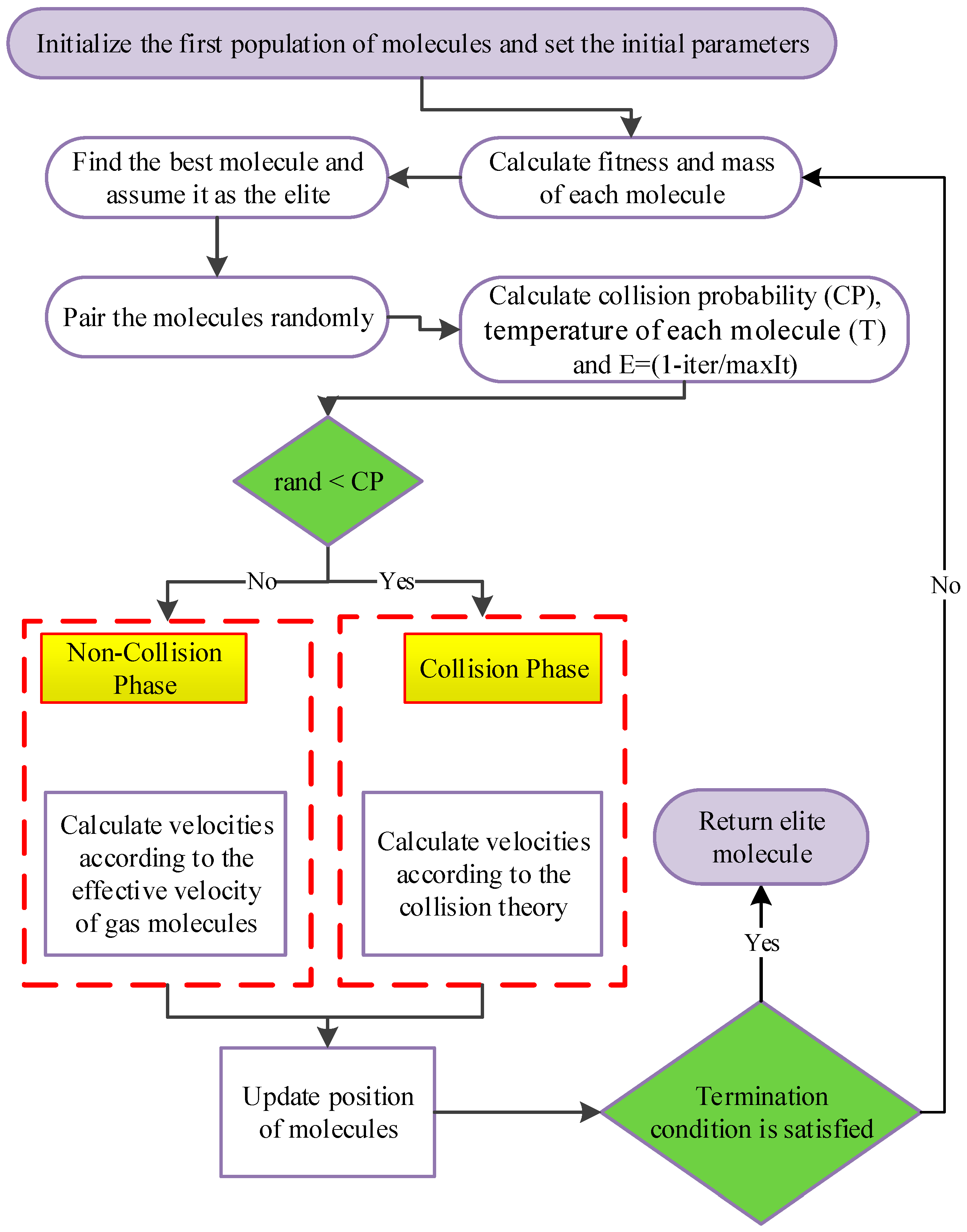
2.1. Mono-Objective IGMM-Based Algorithm

Ideal gas molecules in an isolated environment, due to the two latent factors of high velocity of ideal gas molecules and their high probability of collision, quickly disperse in different directions and cover the entire confined space.

Recently, the IGMM algorithm has been introduced as a meta-heuristic optimization method, and its application in solving numerical and engineering optimization problems has been evaluated [26,27,28]. It uses the equations governing the elastic collision and speed equation of ideal gas molecules to determine the new position of the gas molecules in each iteration. The different steps of the IGMM algorithm can be summarized as follows:

Step 1: Generate the initial population uniformly.

Step 2: Evaluate molecules and calculate masses using Equation (1):

$${\mathrm{m}}_{\mathrm{i}}=\frac{1}{\mathrm{fit}\left(\mathrm{i}\right)}/\frac{1}{\sqrt{\sum \left({\mathrm{fit}}^2\left(\mathrm{i}\right)\right)}}$$

(1)

where ${\mathrm{m}}_{\mathrm{i}}$ shows the mass of the $\mathrm{i}$-th molecule and $\mathrm{f}\mathrm{i}\mathrm{t}\left(\mathrm{i}\right)$ indicates the fitness of the $\mathrm{i}$-th molecule.

Step 3: Determine collision probability (CP) based on Equation (2) and pair molecules, avoiding repetition.

$$\mathrm{CP}=1-\exp \left(-\propto \times \mathrm{i}\mathrm{t}\mathrm{e}\mathrm{r}\right)$$

(2)

In Equation (2), $\mathrm{i}\mathrm{t}\mathrm{e}\mathrm{r}$ is the current iteration and $\propto$ regulates the variation of the collision probability and is set to 0.63, as recommended in [29].

Step 4: According to the collision probability, the new velocity and position of each molecule will be calculated as follows:

Step 4.1. In the collision phase, new post-collision velocities are calculated using Equations (3) and (4). In this case, the molecule with the larger mass is assumed to be stationary and the lighter one moves. The initial velocity of the moving molecule is obtained using relation $∆\mathrm{x}=\mathrm{v}∆\mathrm{t}$ (for $∆\mathrm{t}=1$) by subtracting the positions of the two molecules.

$${{(\mathrm{v}}_1^{\mathrm{d}})}^{\prime }=\frac{\left({\mathrm{m}}_1-\mathrm{E}{\mathrm{m}}_2\right)}{{\mathrm{m}}_1+{\mathrm{m}}_2}\times {\mathrm{v}}_1^{\mathrm{d}}$$

(3)

$${{(\mathrm{v}}_2^{\mathrm{d}})}^{\prime }=\frac{(1+\mathrm{E}){\mathrm{m}}_1}{{\mathrm{m}}_1+{\mathrm{m}}_2}\times {\mathrm{v}}_1^{\mathrm{d}}$$

(4)

$\mathrm{d}$ shows the optimization problem’s dimension, and parameter $\mathrm{E}$ is defined as a variable based on the following linear equation.

$$\mathrm{E}=1-\left(\frac{\mathrm{i}\mathrm{t}\mathrm{e}\mathrm{r}}{\mathrm{m}\mathrm{a}\mathrm{x}\mathrm{I}\mathrm{t}}\right)$$

(5)

where $\mathrm{i}\mathrm{t}\mathrm{e}\mathrm{r}$ and $\mathrm{m}\mathrm{a}\mathrm{x}\mathrm{I}\mathrm{t}$ show current and the maximum iterations, respectively. A new position can be computed using Equations (6) and (7):

$$\left({\mathrm{x}}_1^{\mathrm{d}}\right)\prime ={\mathrm{x}}_2^{\mathrm{d}}+\mathrm{r}\mathrm{a}\mathrm{n}\mathrm{d}\times {{(\mathrm{v}}_1^{\mathrm{d}})}^{\prime }$$

(6)

$$\left({\mathrm{x}}_2^{\mathrm{d}}\right)\prime ={\mathrm{x}}_2^{\mathrm{d}}+\mathrm{r}\mathrm{a}\mathrm{n}\mathrm{d}\times {{(\mathrm{v}}_2^{\mathrm{d}})}^{\prime }$$

(7)

where ${\mathrm{x}}_2^{\mathrm{d}}$ shows the position of the stationary molecule before the collision, and accordingly, ${{(\mathrm{x}}_1^{\mathrm{d}})}^{\prime }$ and ${{(\mathrm{x}}_2^{\mathrm{d}})}^{\prime }$ indicate the new positions after the collision.

Step 4.2. In the no-collision phase, the new velocity is determined using Equation (8).

$${\mathrm{v}}_{\mathrm{i}}^{\mathrm{d}}=\sqrt{\frac{\mathrm{k}{\mathrm{T}}_{\mathrm{i}}}{{\mathrm{m}}_{\mathrm{i}}}}$$

(8)

where the Boltzmann constant ($\mathrm{k}$) is assumed to be opposite to the number of molecules, and the new temperature of each molecule is defined using Equation (9), while the initial temperature is set to 1000.

$${\mathrm{T}}_{\mathrm{i}}^{\prime }={\mathrm{T}}_{\mathrm{i}}-1/{\mathrm{m}}_{\mathrm{i}}$$

(9)

Finally, the new position is obtained by

$$\left({\mathrm{x}}_{\mathrm{i}}^{\mathrm{d}}\right)\prime ={\mathrm{x}}_{\mathrm{i}}^{\mathrm{d}}+\mathrm{r}\mathrm{a}\mathrm{n}\mathrm{d}\times {{(\mathrm{v}}_{\mathrm{i}}^{\mathrm{d}})}^{\prime }$$

(10)

Step 5: The convergence criterion is checked, and if not converged yet, steps 2 to 4 are repeated.

The results were compared with those based on several well-known optimization algorithms, which showed the significance of the proposed IGMM algorithm in terms of both the accuracy and the number of function evaluations towards the optimal solutions [29]. Figure 1 shows the flowchart of the IGMM algorithm.

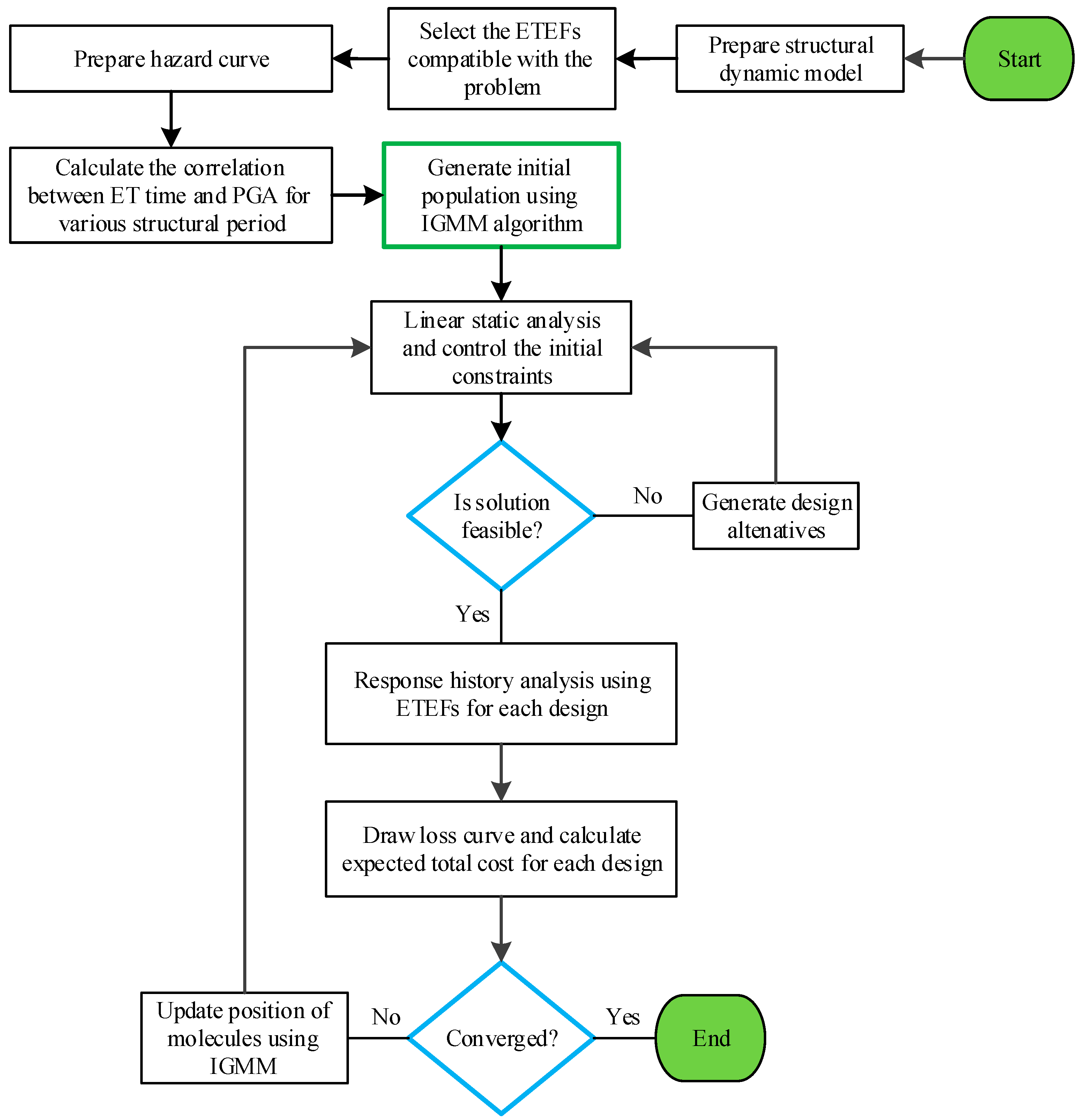
2.2. IGMM-Based Multi-Objective Optimization Algorithm

Multi-objective optimization problems commonly contain terms in conflict with each other. One procedure combines all the objectives into a single one and attempts to solve the problem using conventional mono-objective optimization algorithms [28,29]. Generating a Pareto-optimal front is another way [30,31,32], where the solution is a set of Pareto-optimal solutions, referred to as non-dominated optimum points. This set represents the best trade-offs between the objectives [33,34].

By extending the basic ideas of IGMM, the aim is to develop a type of Multi-Objective IGMM-based algorithm, referred to as MO-IGMM, to be described later. First, an archive of non-dominated designs is gradually built and equipped to finally reach a predefined size. It allows its members to renovate through the optimization procedure and build upon the number of its associates until a maximum diverse size is reached. It then replaces its members with more enhanced and uniformly distributed solutions. The probability of collision of each molecule from the current set in the population is calculated. In the event of a collision, the stationary molecule is selected from the low-density region of the archive molecules. Then, the new velocity and position of the selected molecule is calculated based on the elastic collision equations. Finally, it approximates the true Pareto-optimal front as closely as possible. Below is how archive molecules are used, updated, and selected during the optimization process to ensure consistent distribution of its members.

A stationary molecule is selected from the least populated area of the determined Pareto front to achieve a uniform Pareto-optimal front. To find the least populated area, the search space is divided into segments. For this purpose, the best and worst objectives of the Pareto-optimal solutions are found at each iteration, and a hyper-cube is built to cover all the solutions. It is then divided into equal sub-hyper-cubes, and a selection operand is carried out based on the Coello et al. suggestion by a Roulette-wheel mechanism with the following probability for each segment [35]:

$$P_i=\frac{c}{N_i}$$

(11)

where c is a constant value greater than one [36,37] and $N_i$ is the number of Pareto-optimal solutions found in the i-th segment. Based on this equation, stationary molecules have a greater chance of being selected from the less populated segments. Moreover, this can allow molecules to migrate around regions faster, improving the Pareto-optimal front’s distribution.

The archive should be updated in each iteration where it may primarily become complete. However, it allows conversion into more enhanced non-dominated solutions during optimization. Therefore, there should be a system to handle the archive. It should be prohibited from entering the archive if a solution is dominated by at least one of the archive members. Suppose a solution dominates any of the Pareto-optimal solutions in the archive. In that case, all of them should be deleted from the archive and replaced with the only accepted non-dominated solution. If the archive is complete, one or more solutions may be deleted from the most populated segments to make room for (a) new solution(s). The ability to assess new points adjacent to their current position is given to enhance the MO-IGMM’s local search. This mechanism is only activated for molecules that are not involved in the collision to avoid unnecessary function evaluations. A detailed explanation of the procedure of MO-IGMM algorithm may be found in [35]. The MO-IGMM procedure is summarized below:

Step 1. Determine the maximum number of iterations, population size, archive size, number of hyper cubes, and initial temperature. In the first iteration of the optimization procedure, the initial temperature is set to a large number.

Step 2. Generate a random population of molecules with a uniform distribution.

Step 3. Evaluate the fitness of each molecule denoted from now on as mass.

Step 4. Find the non-dominated solutions.

Step 5. Update the archive with more governing non-dominated solutions obtained.

If the archive is complete, one or more solutions will be deleted from the most populated segments to accommodate the archive’s new solution(s).

Step 6. Obtain the solution range and define hyper-cubes on their basis.

Step 7. Calculate values of $CP$ and $E$ using $CP=iter/MaxIt$ and $E=1-CP$.

Step 8. Update the velocity and position of each molecule.

Step 8.1. If $rand\le CP$, the moving molecule will collide with a stationary one selected from the archive.

Step 8.2. If $rand>CP$, the collision does not occur, and new velocity and position of the corresponding molecule will be found based on the effective velocity of gas.

Step 9. A new solution is generated around the current position of a molecule using Equation (12) to avoid local optima:

$$x_n=x_i^{\prime }\times 0.1\times unifrnd(-\mathrm{1,1},1,varsize)\times E$$

(12)

where $x_n$ is the position of the neighboring molecule and $x_i^{\prime }$ is the position of the new molecule in the current iteration. The new molecule will then be replaced by the neighboring molecule if dominated.

Step 10. Find the non-dominated solutions and then update the archive and hyper-cubes.

Step 11. Check the convergence criteria. If the algorithm is not converged, the optimization process is repeated from steps 7 to 11.

3. Endurance Time Method

As a response history analysis, the Endurance Time (ET) method can measure the structural responses such as maximum displacements, inter-story drift ratios, and stresses in time steps while the intensity of the applied accelerograms is increasing. Excitation in these artificial acceleration functions begins at a low intensity and steadily increases until structural failure occurs. Moreover, this allows structural responses to be tracked through a wide range of intensities [4]. The ET method does, in fact, link analysis time to excitation intensity. The concept of the acceleration reaction spectrum is helpful in ET for characterizing excitation intensity. ET excitation functions (ETEFs) are optimized while each time window, from zero to a particular time, generates a response spectrum that fits a template spectrum with a varying scale factor [38]. Many studies have shown that the currently available ETEFs provide accurate structural response estimates at various excitation intensities with minimal computational effort [24,39]. Various ET acceleration functions are now freely accessible on the ET method’s website [40]. In this investigation, “ETA40h” series acceleration functions are utilized as the basic accelerogram. The template spectrum of this series is the average response spectrum of seven ground motions recorded on soil type C. These motions are selected from a set of 20 earthquake records listed in FEMA440 [41]. According to Estekanchi et al., three acceleration functions in this series, which have different starting points for optimization, can reduce the random scatter effects in the results [22].

In the ET method, the value of the required engineering demand parameter (EDP) (e.g., drift for each story) is found over time. Then, the maximum absolute value of the EDP in the time interval [0, t] is plotted against the analysis time t. The x-coordinate axis of an ET curve is analysis time, but it is not common and, occasionally, can be confusing to evaluate and express seismic performance with time. Therefore, substituting a standard parameter such as peak ground acceleration (PGA) or return period for a time in the evaluation and expression of the performance of the structures is essential. A correlation between ET analysis time and the stated standard parameter should be determined [41]. In this research, the problem of correlation between time and the PGA has been used.

4. Design Based on the Life-Cycle Cost

To optimally design the desired structure based on the Life-Cycle Cost, the sum of the initial construction cost and those caused by probable earthquakes during the structure’s useful period for a lifetime is considered as the total Life-Cycle Cost.

We will show that the ET analysis provides a suitable tool for performing acceptable-volume economic calculations on different design alternatives. The initial construction cost and the expected earthquake loss during the structure lifetime are usually two essential parameters for making decisions [1]. A severe obstacle in evaluating the cost of the earthquake loss is to estimate the structure response against the ground motion under different intensity levels. Different researchers have proposed different simplified seismic analysis methods to overcome the immense computational effort required to evaluate a large number of different designs. However, the cost evaluation has been used so far for comparative studies among a limited number of design alternatives. Researchers have only recently considered the direct use of the Life-Cycle Cost in the design process [1,42]. The total Life-Cycle Cost of the structure $C_{LC}$ can be written as the sum of the initial cost $C_{IN}$, which is a function of the design vector s and the present value of the lifetime cost $C_L$, which is a function of the structure lifetime t and the design vector s as in Equation (13) [1]. The details of which will be explained next.

$${C_{LC}\left(t.s\right)=C}_{IN}\left(s\right)+C_L(t.s)$$

(13)

4.1. Initial Cost

The initial cost is usually the cost of constructing a new structure or retrofitting an existing one. In the design example of a new 3D moment frame RC structure being investigated, the initial cost is related to the costs of land, building materials, and the labor force needed to construct the structure. Since the costs of land and other non-structural elements are the same for all the design alternatives, they can be omitted from the total cost calculations. Therefore, the initial cost can be calculated based on Equation (14), taking into account the reinforcement steel, concrete, and framework costs.

$$C_{IN}={\sum }_{i=1}^{n_b+n_c}\left\{C_c{b}_i{h}_i+C_s{A}_{si}+2C_f(b_i+h_i)\right\}{l}_i$$

(14)

where $C_c$, $C_s$, and $C_f$ are the unit costs of concrete, steel reinforcement, and formwork, respectively, with corresponding values, respectively, of 735 USD/m³, 7.1 USD/kg, and 54 USD/m² [42]. $A_{si}$ is the section area of the steel reinforcement (for beams, it is equal to the sum of the section areas of the upper and lower bars), and $b_i$, $h_i$, and $l_i$ are the member section dimensions, breadth, height, and length, respectively.

4.2. Lifetime Cost

This part includes the structural costs sustained during the useful period of its lifetime. These costs are generally all-inclusive and include losses due to natural and unnatural disasters. However, in the present research, only the seismic losses caused by earthquakes have been considered lifetime costs. According to the existing technical literature, different limit states have been used considering the inter-story drift and the acceleration of the stories. These limit states (and the resulting loss) are due to the performance of the structural and non-structural elements.

The lifetime costs of a structure during its useful period may be due to many factors, including natural and unnatural disasters such as seismic hazards. They may be characterized as the loss of contents itemized by the maximum inter-story drift and the floor acceleration, the damage repair cost, the loss of rental cost, the income cost, the cost of injuries, and the cost of human fatalities [12,43]. As for an economic assessment of these losses, a correlation is used according to limit states suggested by Ghobarah [44] for maximum inter-story drift ratios and a work by Elenas and Meskouris [45] for the maximum floor accelerations, as shown in

Table 2. IDR and maximum floor acceleration limits for different damage states.

Performance Level	Damage States	Drift Ratio Limit (%) Ghobarah [44]	Floor Acceleration Limit (g) Elenas and Meskouris [46]
I	None	$∆\le 0.1$	$a_{floor}\le 0.05$
II	Slight	$0.1\le ∆\le 0.2$	$0.05\le a_{floor}\le 0.1$
III	Light	$0.2\le ∆\le 0.4$	$0.1\le a_{floor}\le 0.2$
IV	Moderate	$0.4\le ∆\le 1.0$	$0.2\le a_{floor}\le 0.8$
V	Heavy	$1.0\le ∆\le 1.8$	$0.8\le a_{floor}\le 0.98$
VI	Major	$1.8\le ∆\le 3.0$	$0.98\le a_{floor}\le 1.25$
VII	Destroyed	$∆>3.0$	$a_{floor}>1.25$

. In general, the maximum inter-story drift ratio (IDR) is used to calculate both structural and non-structural damages, and maximum floor acceleration ($a_{floor}$) is used to justify the loss of contents [43]. In order to create a continuous relationship between the damage states and costs, a piecewise linear relation is assumed.

As mentioned earlier, the lifetime cost of the structure is a combination of different components. The limit state cost ($C_{ls}^i$), for the i-th limit state, may be characterized as follows:

$$\begin{gathered} C_{ls}^i=C_{dam}^i+C_{con}^i+C_{ren}^i+C_{inc}^i+C_{inj}^i+C_{fat}^i \\ {C}_{con}^i=C_{con}^{i.\theta }+C_{con}^{i.acc} \end{gathered}$$

(15)

where $C_{dam}^i$ is the damage repair cost; $C_{con}^{i.\theta }$ is the loss of contents cost due to the interstory-drift; $C_{con}^{i.acc}$ indicates the loss-of-contents cost due to the acceleration in each floor; $C_{ren}^i$ is the loss of rental cost; $C_{inc}^i$ signifies the cost of income loss; $C_{inj}^i$ is the injuries cost and $C_{fat}^i$ indicates the cost of human fatalities. The formulae to calculate each cost component are shown in

Table 3. Formulas for cost calculation in monetary units (based on Dollars or Euros) [1].

Cost Category	Calculation Formula	Basic Cost
Damage/repair ($C_{dam}$)	Replacement cost × floor area × mean damage index	1500 $\mathrm{M}\mathrm{U}/{\mathrm{m}}^2$
Loss of content ($C_{con}$)	Unit content cost × floor area × mean damage index	500 $\mathrm{M}\mathrm{U}/{\mathrm{m}}^2$
Rental ($C_{ren}$)	Rental rate × gross leasable area × loss of function	10 $\mathrm{M}\mathrm{U}/\mathrm{m}\mathrm{o}\mathrm{n}\mathrm{t}\mathrm{h}/{\mathrm{m}}^2$
Income ($C_{inc}$)	Rental rate × gross leasable area × down time	2000 $\mathrm{M}\mathrm{U}/\mathrm{y}\mathrm{e}\mathrm{a}\mathrm{r}/{\mathrm{m}}^2$
Minor Injury ($C_{inj.m}$)	Minor injury cost per person × floor area × occupancy rate × expected minor injury rate	2000 $\mathrm{M}\mathrm{U}/\mathrm{p}\mathrm{e}\mathrm{r}\mathrm{s}\mathrm{o}\mathrm{n}$
Serious Injury ($C_{inj.s}$)	serious injury cost per person × floor area × occupancy rate × expected serious injury rate	$2\times {10}^4$ $\mathrm{M}\mathrm{U}/\mathrm{p}\mathrm{e}\mathrm{r}\mathrm{s}\mathrm{o}\mathrm{n}$
Human fatality ($C_{fat}$)	Human fatality cost per person × floor area × occupancy rate × expected death rate	$2.8\times {10}^6$ $\mathrm{M}\mathrm{U}/\mathrm{p}\mathrm{e}\mathrm{r}\mathrm{s}\mathrm{o}\mathrm{n}$

Occupancy rate 2 $\mathrm{p}\mathrm{e}\mathrm{r}\mathrm{s}\mathrm{o}\mathrm{n}/100 {\mathrm{m}}^2$.

. The values of the mean damage index, loss of function, downtime, expected minor injury rate, expected serious injury rate, and expected death rate used in this study are based on ATC-13 [47] and restated in FEMA-227 [46].

Table 4. Damage state parameters for cost calculations [1].

Limit State	FEMA-227 [46]				ATC-13 [47]
	Mean Damage Index (%)	Expected Minor Injury Rate	Expected Serious Injury Rate	Expected Death Rate	Loss of Function (%)	Down Time (%)
None	0	0	0	0	0	0
Slight	0.5	3.0 × 10−5	4.0 × 10−6	1.0 × 10−6	0.9	0.9
Light	5	3.0 × 10−4	4.0 × 10−5	1.0 × 10−5	3.33	3.33
Moderate	20	3.0 × 10−3	4.0 × 10−4	1.0 × 10−4	12.4	12.4
Heavy	45	3.0 × 10−2	4.0 × 10−3	1.0 × 10−3	34.8	34.8
Major	80	3.0 × 10−1	4.0 × 10−2	1.0 × 10−2	65.4	65.4
Destroyed	100	4.0 × 10−1	4.0 × 10−1	2.0 × 10−1	100	100

provides corresponding parameters for each damage state. The method, with no limitation, has the capability of incorporating detailed calculations on cost components.

The expected LCC of the building is computed by summing up the present values of the annual damage costs throughout its lifetime. For convenience, the detailed procedure to calculate $C_L^i$ for the structure, using the ET method, is depicted in Figure 2.

If the useful structural lifetime period is assumed to be 50 years, Equation (16) can be used, in the present time, to estimate the loss cost to different structural components in its useful lifetime period.

$$C_L^i(t.s)=\frac{1-\exp (-\vartheta t)}{\vartheta }\times C_{ls}^i$$

(16)

where $C_L^i(t.s)$ is the cost of the i-th damage component during the useful structural lifetime period t and ϑ is the annual discount rate (3% in this research [4]). The structure’s lifetime cost due to damage will be calculated by adding the computed present cost for each damage component. According to Equation (13), the total Life-Cycle Cost is equal to the total initial construction cost and the present annual cost of a useful structural lifetime period.

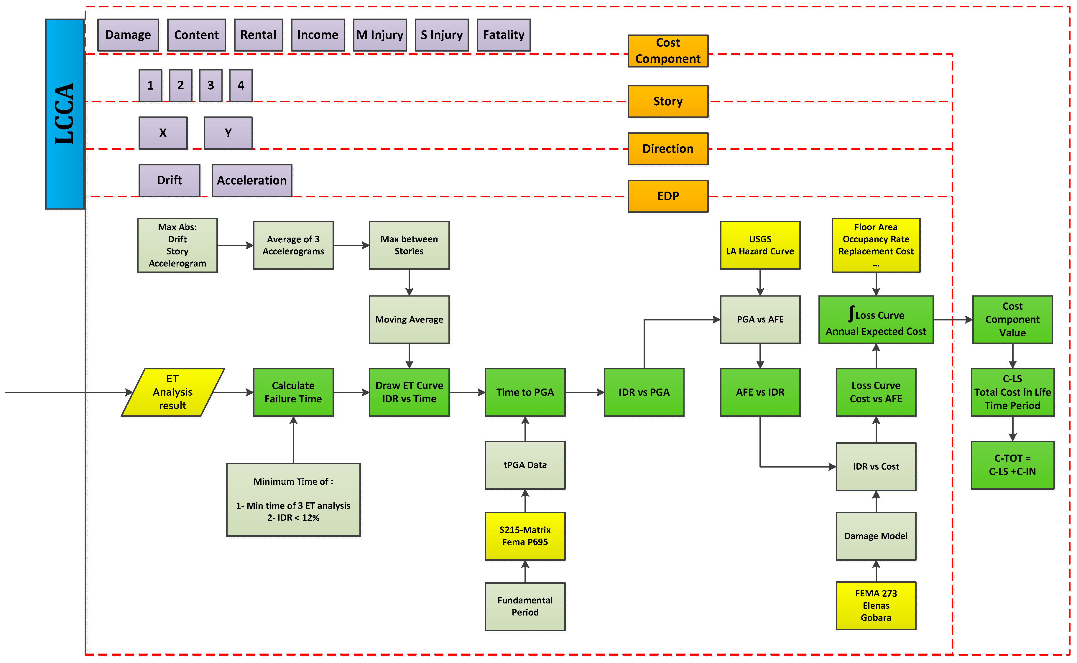
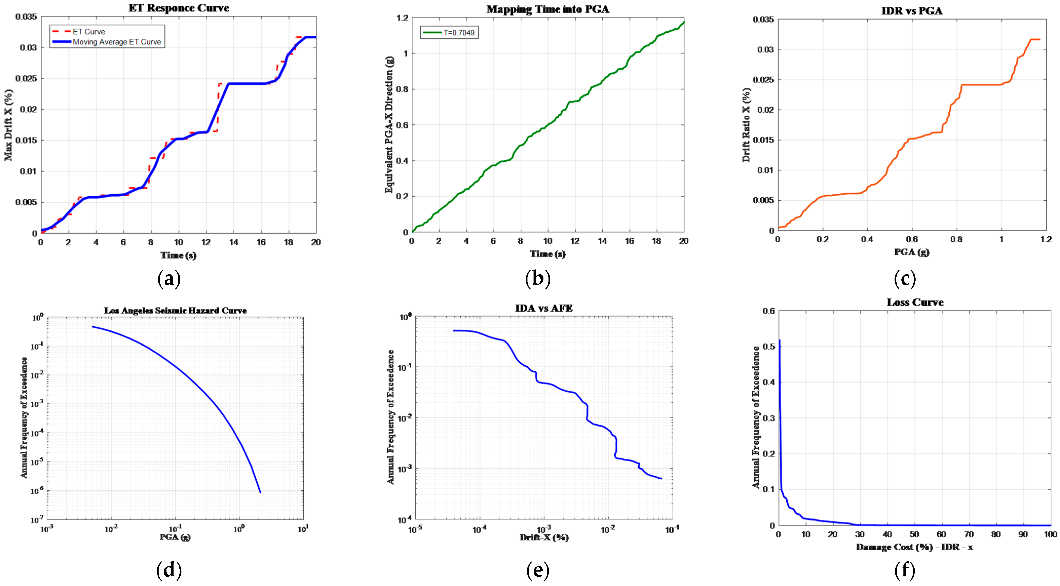
4.3. LCC Calculations Based on the ET Approach

The lifetime cost assessment in the optimization process steps through the results found from the ET analysis and requires a specific procedure. The steps are as follows.

Step 1. In this step, the history of the engineering demand parameters, including the maximum inter-story drift and acceleration of the stories over time, are found through the ET analysis, presented in the form of an ET response curve, and smoothed by fitting a curve on it. Figure 3a shows the ET response curve related to the history of the maximum inter-story drift for an assumed structure. It is worth mentioning that before drawing Figure 3a, the amounts of the responses are extracted for all the stories, and their maximum absolute values are determined.

This process is carried out for all the required demand parameters, including the maximum drift in the Y direction and the maximum acceleration in different directions.

Step 2. In this step, mapping time (in the ET curve) to PGA is carried out based on the procedure explained in [37], and the curve of PGA versus time is drawn based on the fundamental period of the structure being studied (Figure 3b).

Step 3. Here, the curve of the response values (e.g., the maximum drift) versus PGA is drawn, which will result in the elimination of the time factor from the relations, and PGA is substituted (Figure 3c).

Step 4. In this step, the hazard curve of the region of the structure under investigation (LA in this research) is drawn based on the information obtained from the USGS site [48]. Figure 3d shows the relation between PGA and Annual Frequency Exceedance (AFE).

Step 5. Here, the relation between the structure response (maximum inter-story drift) and the AFE is created, and the PGA is omitted from the relations (Figure 3e).

Step 6. In this step, the damage model is made, and the relation between the damage and the AFE is drawn. This step is for different damage components, including the costs of repairs, losing contents due to inter-story drift, losing contents due to the acceleration of stories, losing rent, losing incomes, cost of injuries, and cost of fatalities, and different damage components are found based on the explanations presented at the beginning of this chapter. Figure 3f shows the loss curve of the repair costs due to the drift in direction X.

The above process is repeated many times in different optimization steps until the algorithm convergence conditions are satisfied and the optimum solution is achieved. As mentioned before, step 4 depends on the region of the structure and does not necessarily need to be repeated in each iteration. Figure 4 shows the flowchart of the optimization cycle.

Next, the optimization process is carried out once single-objectively using the IGMM algorithm and bi-objectively using the MOIGMM algorithm.

5. Numerical Example

5.1. Structural Model

In this research, a numerical structural model has been used, considering nonlinear material properties and deterioration. The structural analyses were carried out using the performance-based earthquake engineering (PBEE) toolbox [49]. The Euro code 8 [50] specifications, together with the works by Fajfar and Eeri [51] and Perus et al. [52], were employed to define moment–rotation relations of the plastic hinges. Some assumptions used in the nonlinear modeling process are as follows:

-

The floor diaphragms are assumed to be rigid in their planes, and the masses and the moments of inertia are lumped at the center of gravity.

-

The elastic elements connect all joints at the story level to the center of mass. They are used to model the rigid diaphragm at the story level, where the mass can be represented in one point. Columns contain the P-delta effect.

-

One-component lumped plasticity elements, consisting of an elastic beam and two inelastic rotational hinges (defined by the moment–rotation relationship), are used to model the beam and column flexural behaviors. The element’s formulation is based on the concept of a point of inflection at the element’s midpoint. The plastic hinge is only used for the main axis bending in beams. For columns, two independent plastic hinges are used for bending about the two principal axes [53].

-

In the present study, the elastic beam-column elements and zero-length-section elements are used to create the model. At each elevation, “rigid” elements linked all of the nodes. The TakedaDAsym uniaxial material, designed in the software OpenSees_1.7.4, is used for plastic hinges in beams and columns [49].

-

A bi-linear or tri-linear relationship is used to model the moment–rotation relationship. When determining the moment–rotation relationship for beams or columns, zero axial force and axial strain due to gravity loads are considered, respectively. After the maximum moment, a linear negative post-capping stiffness is assumed.

-

The gravity load was modeled on beams as a uniformly distributed load and on columns as point loads. The self-weight of the slab and beams and the permanent load on the slab result in an evenly distributed load on the beams. Only the self-weight of columns is modeled using the point loads at the top of the columns.

Moment–rotation plastic hinges, which were considered at both ends of the structural members, were used to model only the nonlinear action of the columns and beams. The moment–rotation interaction was treated as tri-linear, with the substance softening after the maximum moment (Figure 5). The three points at the increasing part of the moment–rotation envelope show the cracking of the concrete (CR), the yielding of reinforcement (Y), and the maximum moment (M). The linear strength degradation is assumed and identified with the point at the near-collapse after the maximum moment is reached (NC). Based on the given parameters and properties such as the geometry of the column cross-section, material strength, longitudinal reinforcement, containment effectiveness factor, amount of steel transfers parallel to the direction of loading, and the axial load resulting from the gravity load, the PBEE toolbox automatically calculates the moment–rotation relationships in the plastic hinges of columns and beams [54].

Further information on the details of the structural design and the preparation of the analytical model may be studied in [49,55].

The structure can be subjected to earthquake excitations in the X and/or in Y direction. The Newmark integrator is used assuming γ = 0.5 and β = 0.25.

5.2. Defining the Optimization Problem

In single-objective optimization, the minimization of the total cost is considered as the objective function. Accordingly, it is required that the design alternatives satisfy certain initial constraints. Columns’ strengths have a reducing trend in the building height, meaning that the dimensions of the upper columns should be equal to or smaller than those of the lower ones. Besides these constraints, all the other code-based constraints regarding the gravity loads should be satisfied too. After these are satisfied for a design alternative, the LCC analysis is performed based on the ET analysis (explained in Section 4.3). To achieve the optimum design, this algorithm generates new designs based on the initial population until the convergence criterion is reached.

The design variables are the details of the beams and columns. In a general state, we include the relative section areas of the lower and upper bars ($\rho$ and ${\rho }^{\prime }$, respectively), beam breadth and height (b and h, respectively), and stirrups’ relative section area and spacing (${\rho }_{sh}$ and s, respectively), among which the latter two are assumed constant in the optimization process. Their values are found based on the seismic design specifications specified in the related codes. To simplify the execution of the final design, the beams’ section breadth at each story level is limited to that of the columns below, and only the beams section height is defined as a discrete variable in the range of 30–60 cm with 5 cm paces. Additionally, the relative section area of the beam’s lower bars is assumed to be half that of the upper bars (more than the minimum permissible value specified in the related codes). Therefore, the design variables in the optimization problem include only the beam section heights and section areas of the upper bars. Additionally, the relative section areas of the beam reinforcement bars are defined discretely considering arrangements of two, three, and four bars 16–25 mm in diameter.

The columns’ details, in a general state, include the relative section area of all the column reinforcement bars (${\rho }_{TOT}$), the column section breadth and height (b and h, respectively), and stirrups’ relative section area and spacing (${\rho }_{sh}$ and s, respectively). Similar to beams, the latter two are found based on the seismic design specifications specified in the related codes. To define the problem discretely and consider construction limitations, column section dimensions and numbers and diameters of the steel bars are shown in

Table 5. Predefined column sections’ properties.

Number	Name	n	$\mathbf{\Phi }$ (mm)	${\mathit{L}}_{\mathit{x}}$ (cm)	${\mathit{L}}_{\mathit{y}}$ (cm)	${\mathit{A}}_{\mathit{s}}$ (cm2)	${\mathit{A}}_{\mathit{g}}$ (cm2)	${\mathit{\rho }}_{\mathit{T}\mathit{O}\mathit{T}}$ (%)
1	C30x30-8T16	8	16	30	30	16.08	900	1.79%
2	C30x30-8T18	8	18	30	30	20.36	900	2.26%
…	…	…	…	…	…	…	…	…
27	C45x45-16T20	16	20	45	45	50.26	2025	2.48%
28	C45x45-16T22	16	22	45	45	60.82	2025	3.00%
…	…	…	…	…	…	…	…	…
65	C60x60-24-22	24	22	60	60	91.23	3600	2.53%
66	C60x60-24-25	24	25	60	60	117.81	3600	3.27%

, from which the optimization algorithm chooses the required values. Column sections have been assumed squares with discrete dimensions that vary with 5 cm paces. The reinforcement bars have 8, 12, and 16 setting arrangements with appropriate clear spacing between the steel bars. In defining the sections, use has been made of 16, 18, 20, 22, and 25 mm diameter bars so that the column section bar ratio lies within the permissible range specified in the related codes.

The studied case is a 3D four-story RC structure with two spans in each direction; in direction X, the span dimensions are both equal to 5 m, and in direction Y, they are 4 and 6 m. The height of the bottom story is 3.5 m, and the height of the other stories is 3.0 m. Twelve column types (6 for stories 1 and 2 and 6 for stories 3 and 4) and 28 beam types (3 for direction X and 4 for direction Y in all different stories) have been considered due to the existing symmetry in the structure. So there are 72 design variables for the problem, including 12 for the column sections, 4 for the beam heights, and 56 for the beam’s upper steel bars (one independent variable for each end of a beam). As mentioned before, these variables can assume only predefined values. Locations of each beam (B1–B7) or column (C1–C6) section on the plan are shown in Figure 6.

5.3. Mono-Objective Optimization

To achieve a design with the slightest variations in the initial cost, first, the structure was designed according to the ACI 318-14 [56] provisions and observing all the existing constraints. Secondly, the range of variations of every design variable in the optimization process was determined based on the Life-Cycle Costs. Accordingly, the permissible values the design variables can assume are provided in

Table 6. Predefined sections properties.

Element	Variable	Permissible Values
Column	Column section	28 first section of Table 1
Beam	Height (cm)	30, 35, 40, 45
Beam	Relative section areas of the upper bars (%)	0.35, 0.5, 0.7, 0.8, 1.0, 1.2, 1.4, 1.6, 2.0

. A non-stationary multi-stage assignment penalty function method is applied similar to that of [57,58,59] to handle constraints.

In this example, the IGMM algorithm was able to find the approximately optimum structure with an initial population of 20 after 30 cycles, which is nearly 1800 time-history analyses (three analyses for each ET response curve based on the combinations of the three pairs of accelerograms).

Table 7. Optimization problem breakdown.

Category	Description
Objective	Minimize sum of the initial construction cost $\left(C_{IN}\right)$ and the expected lifetime cost $\left(C_L\right)$ of the structure.
Constraints	1. The selected sections for columns in each story cannot be weaker than those in the upper story.
	2. All code-based limitations imposed by the ACI318-14 design recommendations must be met.
	3. Inter-story drift ratio limits at both operational and ultimate levels must be maintained.
Design Variables	Predefined sections from Table 6.

outlines a breakdown of the optimization problem, the constraints, and the design variables involved.

To compare the performance of the proposed algorithm, we also used the Genetic Algorithm (GA) and Particle Swarm Optimization (PSO) algorithms, which are considered state-of-the-art optimization techniques, alongside the IGMM algorithm.

Table 8. Parameter settings for IGMM, PSO, and GA.

Parameter	IGMM	PSO [60]	GA [60]
Population Size	20	20	20
Max Iterations	100	100	100
Crossover Rate	N/A	N/A	0.9
Mutation Rate	N/A	N/A	0.001
Start Weight	N/A	0.9	N/A
End Weight	N/A	0.4	N/A
Cognitive Component	N/A	1	N/A
Social Component	N/A	3	N/A
Initial Temperature	1000	N/A	N/A
Cooling Schedule	Linear Cooling	N/A	N/A
Selection Mechanism	N/A	N/A	Roulette Wheel Selection
Mutation Mechanism	N/A	N/A	Random Perturbation
Velocity Limits	N/A	[−1, 1]	N/A
Termination Condition	Max Iterations	Max Iterations	Max Iterations
Initialization Method	Random Initialization	Random Initialization	Random Initialization

summarizes the parameter settings for all algorithms, which were chosen based on recommendations from the literature.

Figure 7 shows the convergence history of the IGMM, PSO, and GA algorithms for the studied problem. The rapid convergence of all algorithms during the initial steps is noteworthy. Among these, the IGMM algorithm demonstrates superior performance with faster convergence compared to GA and PSO. The GA algorithm follows, showing better performance than PSO but not matching IGMM’s efficiency. PSO, while effective, has a slower convergence rate in comparison to IGMM and GA.

In seismic design, the traditional approach often adheres to force-based methods as specified by design standards like ACI 318-14 for reinforced concrete structures. These standards typically focus on ensuring that structural components can withstand the forces induced by seismic events. The steps involved in the traditional design process are

• Load calculation based on ASCE 7 and determination of the base shear force using seismic hazard maps and building response factors.
• Preliminary sizing and performing of the initial sizing of structural elements (beams, columns, etc.) to resist the calculated seismic loads.
• Checking for compliance with strength and stiffness requirements.
• Structural analysis using linear static analysis to determine internal forces and moments. In this step, we ensure that all structural elements meet the required safety margins against yielding and buckling.
• Design iteration and adjustment of element sizes and configurations iteratively to optimize material usage while maintaining safety. In this step, we verify the design through detailed checks, such as ensuring proper detailing of reinforcement in concrete structures.

Figure 8a compares the response curves of the maximum inter-story drift of the ET analysis of a structure designed based on the ACI318-14 and the optimum structure designed based on the Life-Cycle Cost, and Figure 8b compares the smoothed curves of the drift versus PGA for both structures. In these curves, the drift values in lower accelerations (which have more occurrence probabilities) are less in the structure optimized based on the Life-Cycle Cost than in the one designed based on codes.

Since drift values directly correlate with the structure damages and the related losses, this parameter can reduce the Life-Cycle Cost.

Figure 8c shows the loss curve due to the drift in direction X of the two structures, one designed based on the ACI318-14 and the other optimized based on the Life-Cycle Cost.

As illustrated in Figure 8c, the solid blue curve related to the latter case demonstrates smaller values. Although the difference may seem negligible, it represents the probable annual loss. When the area under this curve is calculated and extended over a 50-year useful lifetime, even a slight reduction can lead to a significant decrease in the expected total loss.

Table 9. Information regarding the column sections for the code-based design structure.

Column Type	Stories 1 and 2	Stories 3 and 4
C1	40x40-12T20	40x40-8T18
C2	40x40-12T20	40x40-8T20
C3	40x40-12T20	40x40-8T20
C4	45x45-12T20	40x40-8T20
C5	40x40-12T20	40x40-8T16
C6	40x40-12T20	40x40-8T20

,

Table 10. Information regarding the beam sections for the code-based design structure.

No.	Story 1	Story 2	Story 3	Story 4
1	40x40-B8-T16	40x40-B6.4-T12.8	40x40-B5.6-T11.2	35x40-B4.9-T4.9
2	40x40-B6.4-T12.8	40x40-B5.6-T11.2	40x40-B5.6-T11.2	35x40-B4.9-T4.9
3	40x40-B8-T16	40x40-B8-T16	40x40-B5.6-T11.2	35x40-B4.9-T4.9
4	40x40-B8-T16	40x40-B6.4-T12.8	40x40-B5.6-T11.2	35x40-B4.9-T4.9
5	40x40-B9.6-T19.2	40x40-B8-T16	40x40-B5.6-T11.2	35x40-B4.9-T4.9
6	40x40-B9.6-T19.2	40x40-B9.6-T19.2	40x40-B6.4-T12.8	35x40-B4.9-T4.9
7	40x40-B8-T16	40x40-B8-T16	40x40-B6.4-T12.8	35x40-B4.9-T4.9
8	40x40-B9.6-T19.2	40x40-B8-T16	40x40-B6.4-T12.8	35x40-B4.9-T4.9
9	40x40-B8-T16	40x40-B6.4-T12.8	40x40-B5.6-T11.2	35x40-B4.9-T4.9
10	40x40-B8-T16	40x40-B8-T16	40x40-B5.6-T11.2	35x40-B4.9-T4.9
11	40x40-B9.6-T19.2	40x40-B9.6-T19.2	40x40-B6.4-T12.8	35x40-B4.9-T4.9
12	40x40-B9.6-T19.2	40x40-B9.6-T19.2	40x40-B6.4-T12.8	35x40-B4.9-T4.9
13	40x40-B8-T16	40x40-B8-T16	40x40-B5.6-T11.2	35x40-B4.9-T4.9
14	40x40-B8-T16	40x40-B6.4-T12.8	40x40-B5.6-T11.2	35x40-B4.9-T4.9

,

Table 11. Information regarding the column sections for the LCCA-based optimum design.

Column Type	Stories 1 and 2	Stories 3 and 4
C1	40x40-12T18	40x40-8T16
C2	45x45-12T20	35x35-8T16
C3	40x40-8T25	40x40-8T22
C4	45x45-12T16	35x35-8T22
C5	40x40-12T16	40x40-8T20
C6	35x35-8T22	35x35-8T18

and

Table 12. Information regarding the beam sections for the LCCA-based optimum design.

No.	Story 1	Story 2	Story 3	Story 4
1	45x40-B9-T18	45x40-B7.2-T14.4	40x35-B4.9-T9.8	35x35-B4.2875-T6.125
2	45x40-B9-T18	45x40-B7.2-T14.4	40x35-B4.9-T9.8	35x35-B4.2875-T8.575
3	45x40-B10.8-T21.6	45x40-B7.2-T14.4	40x40-B5.6-T11.2	35x40-B4.9-T7
4	45x40-B12.6-T25.2	45x40-B12.6-T25.2	40x40-B8-T16	35x40-B5.6-T11.2
5	45x45-B10.125-T20.25	45x45-B8.1-T16.2	40x35-B5.6-T11.2	35x35-B4.9-T9.8
6	45x45-B10.125-T20.25	45x45-B10.125-T20.25	40x35-B4.9-T9.8	35x35-B4.2875-T4.2875
7	45x40-B12.6-T25.2	45x40-B6.3-T9	40x35-B4.9-T9.8	35x35-B4.2875-T6.125
8	45x40-B7.2-T14.4	45x40-B6.3-T9	40x35-B4.9-T7	35x35-B4.2875-T6.125
9	45x40-B12.6-T25.2	45x40-B12.6-T25.2	40x40-B8-T16	35x40-B5.6-T11.2
10	45x40-B9-T18	45x40-B7.2-T14.4	40x40-B6.4-T12.8	35x40-B5.6-T11.2
11	45x35-B7.875-T15.75	45x35-B7.875-T15.75	40x35-B4.9-T9.8	35x35-B4.2875-T4.2875
12	45x35-B9.45-T18.9	45x35-B6.3-T12.6	40x35-B5.6-T11.2	35x35-B4.2875-T6.125
13	45x35-B9.45-T18.9	45x35-B7.875-T15.75	40x35-B7-T14	35x35-B4.2875-T6.125
14	45x35-B9.45-T18.9	45x35-B5.5125-T7.875	40x35-B4.9-T7	35x35-B4.2875-T4.2875

present the comparative results regarding the sections for both structures.

As shown in

Table 13. Comparative information regarding the details of initial cost.

Initial Cost Components	Traditional Design (USD)	LCC-Based Optimal Design (USD)	Percentage of Variation
Column Reinforcement	13,433	12,961	−4%
Column Concrete	18,931	17,173	−9%
Column Formwork	9790.2	9595.8	−2%
Beam Reinforcement	42,689	43,527	+2%
Beam Concrete	24,933	27,451	+10%
Beam Formwork	15,228	15,595	+2%
Sum	125,004	126,302	+1%

, the initial cost has increased from 125,004 USD in the design based on conventional codes to 126,302 USD in the design based on the Life-Cycle Cost. And, as shown in

Table 14. Comparative information regarding the details of the Life-Cycle Cost.

Lifetime Cost Components	Traditional Design (USD)	LCC-Based Optimal Design (USD)	Percentage of Variation
$C_{dam}$	1.42 × 105	1.21 × 105	−15%
$C_{con}^{\theta }$	47,408	40,171	−15%
$C_{con}^{acc}$	58,914	59,981	+2%
$C_{ren}$	637.49	538.41	−16%
$C_{inc}$	1.28 × 105	1.08 × 105	−16%
$C_{injM}$	71.728	55.702	−22%
$C_{injS}$	223.76	204.26	−9%
$C_{fat}$	19,937	15,915	−20%
Sum	397,192	345,865	−13%

, the costs of the useful lifetime have decreased from 397,192 USD in the code-based design to 345,865 USD in the Life-Cycle Cost-based design. Therefore, in general, only a 1% increase in the initial cost will result in a 13% reduction in the useful period of lifetime costs and a total 10% reduction in the total Life-Cycle Cost of the structure being studied.

The graphical representation of the information provided in the tables is shown in Figure 9. It is worth mentioning that the short permissible ranges for the variations of each design variable and also the discrete space of the problem and variables have caused some limitations in the reduction in the Life-Cycle Costs.

Table 13, Table 14 and

Table 15. Comparative information regarding the details of total Life-Cycle Cost.

Total Cost	Initial Cost (USD)	Lifetime Cost (USD)	Total Life-Cycle Cost (USD)
Traditional Design	1.25 × 105	3.97 × 105	5.22 × 105
LCC-Based Optimal Design	1.26 × 105	3.45 × 105	4.71 × 105
Percentage of Improvement	+1%	−13%	−10%

present the comparative information regarding the details of the lifetime period and initial costs; the percent variation in each cost parameter due to optimization is also shown in each table. The comparative three first periods and mode shapes of the code-based and LCCA-based optimum design are also provided in

Table 16. Comparative Eigenvalue results of the code-based and LCCA-based design.

	Code Based Design			LCCA-Based Design
	First Mode (s)	Second Mode (s)	Third Mode (s)	First Mode (s)	Second Mode (s)	Third Mode (s)
Period	0.736	0.730	0.602	0.722	0.693	0.569
Mode shape	UX	UY	RZ	UX	UY	RZ
Story 1	0.4563	0.4535	0.4669	0.2986	0.3031	0.2247
Story 2	0.7051	0.7014	0.7162	0.5667	0.5716	0.4242
Story 3	0.8968	0.8954	0.9046	0.8205	0.8252	0.5983
Story 4	1	1	1	1	1	1

.

In Table 13, the initial cost of the structure has been recorded for the two cases of LCC-based optimal design and Traditional design. As mentioned in Section 4, the initial cost of the structural components includes the cost of reinforcement, concrete and formwork, which are shown in Table 13. The breakdown for structural components, including beams and columns, has been specified. Due to the reduction in column sections and the increase in beam sections in the optimal design, the initial costs related to columns for reinforcement, concrete and formwork are reduced by 4, 9, and 2 percent, respectively, whereas for beams, there is an increase by 10, 2, and 2 percent, respectively. In total, the LCC-based optimal design will cause a cost increase by 1% compared to the traditional design.

The comparison of the life-cycle costs of the structure can be seen in Table 14. The important point is the positive effect of the LCC-based optimal design in reducing life-cycle costs compared to traditional design. The greatest impact on reducing the costs of the life cycle of the structure is on $C_{injM}$ at 22%, followed by $C_{fat}$, $C_{ren}$ and $C_{inc}$ at 20, 16 and 16%, respectively. The comparison of the total initial costs and the life-cycle costs of the structure for the LCC-based optimal design and traditional design in Table 15 shows that with only 1 percent increase in the initial costs for the structure, the life-cycle costs of the structure can be reduced by 13 percent, with a reduced total life-cycle cost of 10 percent. Thus, the cost of the entire life cycle of the structure shows a decrease from 5.22 × 10⁵ dollars to 4.71 × 10⁵ dollars.

5.4. Multi-Objective Optimization

The initial or total cost of a structure alone may not prepare comprehensive data on the structure’s performance in a real-life design problem. Many contradictory and often inconsistent requirements should be considered concurrently to arrive at a rational design in practical decision-making issues. As a result, a consistent decision-making process necessitates detailed knowledge about design options from which a designer chooses the one that best balances conflicting goals. This knowledge can be better demonstrated in a Pareto front of design alternatives with optimized initial costs and Life-Cycle Costs concurrently. The two most critical metrics for decision-making are generally the initial construction cost and the expected cost over the structure’s lifetime. Multi-objective optimization procedures can solve the optimization problem and achieve specific Pareto-optimal designs. The multi-objective algorithm generates a collection of optimal designs for a wide range of alternatives. The key feature of the Pareto-optimal set is that no change in one objective is possible without deterioration in other objectives.

The structure’s initial cost and lifetime cost are the two different objectives in this multi-objective optimization problem. The discrete optimization problem is solved using the multi-objective ideal gas molecular movement (MOIGMM) algorithm. The algorithm’s ability to solve multi-objective optimization problems in a computationally capable manner has been demonstrated by its use in engineering problems [34]. The initial cost $C_{IN}$ and the expected lifetime cost $C_L$ of the structure are the first and second objectives, respectively, and thus, the optimization problem can be set as

$$\begin{gathered} {Minimize}_{s\in F}\left[C_{IN}\left(s\right),C_L\left(s.t\right)\right] \\ Subject to g_j\left(s\right)\le 0 j=\mathrm{1,2},3,\dots ,k \end{gathered}$$

(17)

where s is the design vector, F is the feasible design space, and k is the number of constraint functions. There are a total of 72 design variables for the problem, including 12 for the column sections, 4 for the beam heights, and 56 for the relative section areas of the beam’s upper steel bars, with one independent variable for each end of a beam. $g_j$ denotes the constraints that candidate design alternatives should meet. One of the constraints is that the selected sections for columns in each story cannot be weaker than those in the upper story. In addition, all code-based limitations imposed by ACI318-14 design recommendations must be met. Moreover, this means that according to prescriptive design requirements, all Pareto-optimal designs would be acceptable. Inter-story drift ratio limits are also set at both operation and ultimate levels. These are controlled using a linear elastic analysis by OpenSees software_1.7.4 [61]. Once the expressed constraints have been met, a nonlinear time-history analysis using the ET method is carried out. The expected lifetime cost due to future seismic hazards is measured using Life-Cycle Cost assessment.

Table 17. Optimization problem breakdown.

Category	Description
Objective	Minimize both the initial construction cost $\left(C_{IN}\right)$ and the expected lifetime cost $\left(C_L\right)$ of the structure.
Constraints	1. The selected sections for columns in each story cannot be weaker than those in the upper story.
	2. All code-based limitations imposed by ACI318-14 design recommendations must be met.
	3. Inter-story drift ratio limits at both operational and ultimate levels must be maintained.
Design Variables	1. Column sections: Predefined sections from Table 9
	2. Beam heights: Permissible values are 30, 35, 40, 45, 50, 55, 60 cm
	3. Relative section areas of the upper bars: Permissible values are 0.35%, 0.40%, 0.45%, 0.50%, 0.60%, 0.65%, 0.70%, 0.75%, 0.80%, 0.85%, 0.90%, 0.95%, 1.00%, 1.10%, 1.20%, 1.30%, 1.40%, 1.50%, 1.60%, 1.80%, 2.00%

lists the objectives, constraints, parameters, and decision variables of the optimization problem. Based on Table 17, each design variable’s variation interval is increased, and the MOIGMM algorithm is allowed to search a broader range to eventually yield a complete Pareto front. After 25 cycles, with an initial population of 20, archive size of 25, and number of sub-cubes equal to 30, this algorithm performed the Pareto front shown in Figure 10.

It is worth noting that each design on a Pareto front that meets a vertical line with a specified distance from the origin (initial cost) is the one with the best performance possible to be built with its initial cost. For instance, Figure 10 shows the optimum design based on a mono-objective optimization and its related initial cost. It reveals that this design has the lowest total cost among those with similar initial costs. As expected, an increase in the range of variations of the design variables will yield points with lower total costs than the solution found in the mono-objective optimization. Furthermore, this figure can be studied as a guide for decision-making to see the reduction trend of the lifetime cost with an increase in the initial cost. This information can assist the decision-makers to choose a design that can create a relative balance between two objective functions. It also shows that in design alternatives with an initial cost of about 147,000 USD, a slight increase in the initial investment can considerably enhance the structural performance and reduce the future costs. It is worth mentioning that the problem space is discrete because the design variables are discrete, and this has created some discontinuities in the obtained Pareto front. It is possible to consider the sum of the initial and lifetime costs as a criterion for choosing a point from among different Pareto front points. This criterion is shown in Figure 6 by drawing the line $C_{IN}+C_{LC}=cte$. Points lying on this line are responses that will have the minimum total Life-Cycle Cost.

Computational Time

Calculating the objective value involves determining both the initial cost ($C_{IN}$) and the expected lifetime cost ($C_L$) for each design vector. This process can be broken down into the following steps:

The initial cost calculation involves summing the costs of all structural components based on the selected sections, heights, and reinforcement areas. This step is relatively quick and typically requires a few seconds per design vector.

Expected lifetime cost calculation involves performing a nonlinear time-history analysis using the ET method. The computational time for this analysis is more significant due to the complexity of the simulations. On average, the time required to perform the ET analysis and estimate the lifetime cost for one design vector is approximately 12 minutes (for three analyses for each ET response curve).

The total computational time for running the MOIGMM algorithm depends on the number of design vectors in the initial population, the number of cycles, and the complexity of the design space. With 20 design vectors and approximately 12 min per vector, the initial population evaluation takes about 4 h. Each cycle involves evaluating new design vectors generated by the algorithm. Assuming that each cycle evaluates a similar number of design vectors, the time required for each cycle is approximately the same as the initial evaluation.

For 25 cycles, the total time would be 25 cycles × 4 h/cycle = 100 h, and the total computational time for one run would be initial evaluation + optimization cycles = 5 h + 100 h = 105 h.

6. Conclusions

The present work inspects the optimum seismic design of a Life-Cycle Cost on a 3D four-story concrete building structure. The implemented means of the research could perform a comprehensive definition of the seismic effects like structural losses, losses to the structural contents, downtime costs, and costs due to injuries and fatalities as quantitative parameters. Using this technique, one could expect the ensued structure to operate satisfactorily during and after the earthquake. The Endurance Time method was employed to proceed with the nonlinear analysis and structural response prediction. It estimates the structural response under different seismic intensities with computation costs substantially lower than the conventional time-history methods. The utilized technique also prepares the means to employ stochastic algorithms for optimization. The mono- and multi-objective optimization technique based on a new IGMM technique, recently proposed by the authors, was employed here. It is based on the molecular movements of an ideal gas and can converge to the global optimum at the early stages of the optimization process. Based on the customary codes of practice, having compared the currently found optimum structural response with those available in the literature, it signifies the approach for minimizing the lifetime costs of complicated structures. The main findings are summarized below:

-

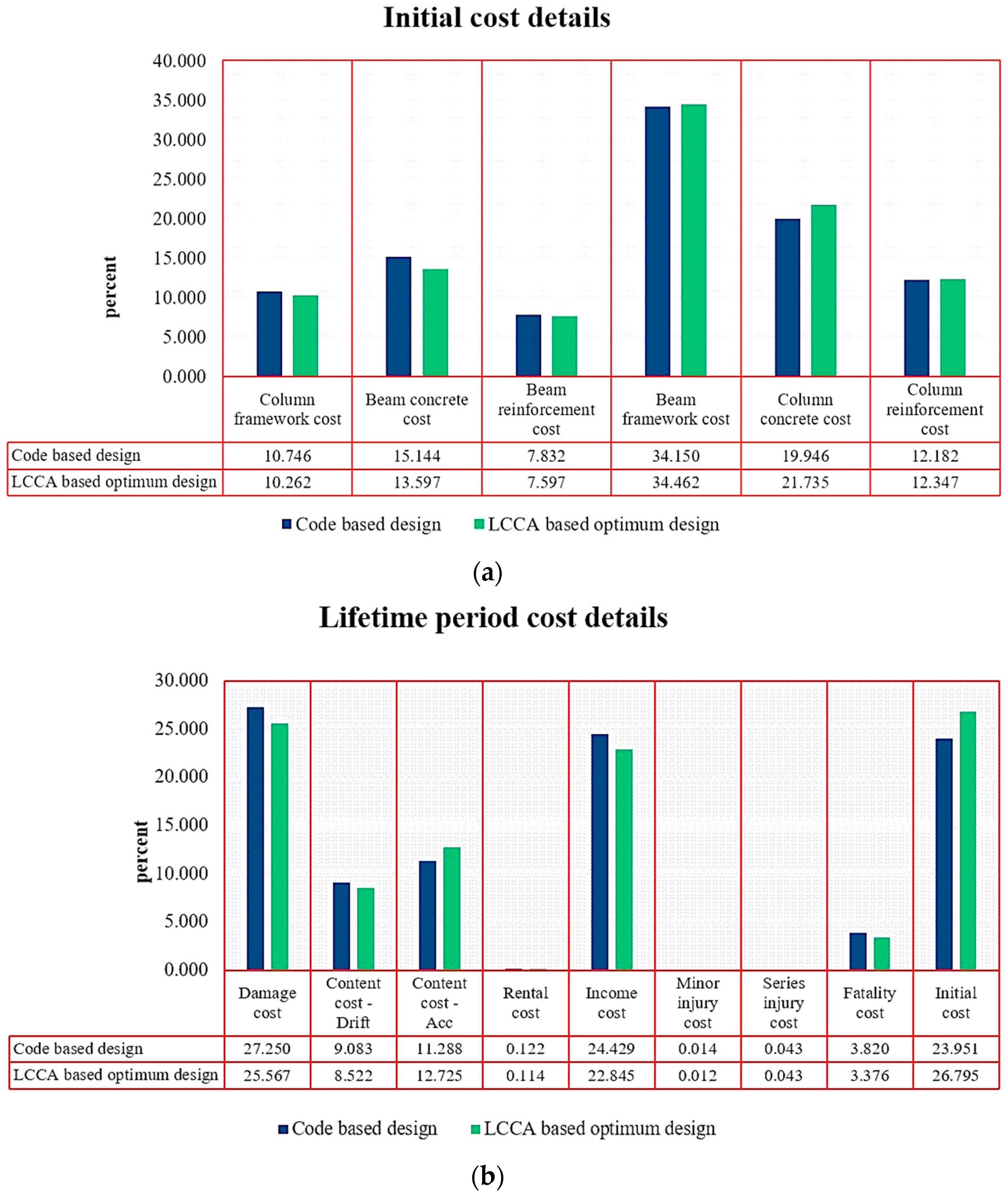
The mono-objective optimization procedure led to a 13% reduction in the useful lifetime costs by merely increasing a 1% initial cost.

-

In total, a 10% reduction in all structural Life-Cycle Costs was attained by mono-objective optimization.

-

The use of LCC-based optimization could cause a significant effect on reducing minor injury, rental, and income costs by 22%, 16%, and 16%, respectively.

-

Using multi-objective IGMM-based optimization resulted in performing a set of optimum responses for the 3D four-story concrete building under study, which could assist engineering designers in making a decision to perform an optimum design.

-

As a result, the accessible methodology here, including the ET method as an analysis tool and IGMM algorithm as an optimizer, provides a numerical tool with a considerable computational saving for the quantitative estimation of the Life-Cycle Cost and the vulnerability assessment of any real-scale reinforced concrete building.

While the proposed framework demonstrates significant improvements in reducing Life-Cycle Costs and enhancing the economic efficiency of seismic designs, there are several limitations and areas for future research. One limitation is the reliance on specific computational models and parameters, which may not fully capture the variability in material properties and construction practices across different regions. Future work could extend the application of this framework to a wider range of building types and materials, incorporating region-specific data to improve accuracy and generalizability. Additionally, the computational demands of the ET method and IGMM algorithm, although reduced compared to traditional methods, still pose challenges for large-scale applications. Future research could explore the integration of advanced machine learning techniques and surrogate models to further optimize computational efficiency and predictive accuracy. Furthermore, while this study focuses on economic and performance criteria, incorporating additional sustainability metrics such as environmental impact and resource efficiency could provide a more holistic approach to seismic design optimization.

References

1. Mitropoulou, C.C.; Lagaros, N.D.; Papadrakakis, M. Life-Cycle Cost Assessment of Optimally Designed Reinforced Concrete Buildings under Seismic Actions. Reliab. Eng. Syst. Saf. 2011, 96, 1311–1331. [Google Scholar] [CrossRef]
2. Varaee, H.; Safaeian Hamzehkolaei, N.; Safari, M. A Hybrid Generalized Reduced Gradient-Based Particle Swarm Optimizer for Constrained Engineering Optimization Problems. J. Soft Comput. Civ. Eng. 2021, 5, 86–119. [Google Scholar]
3. Noori, F.; Varaee, H. Nonlinear Seismic Response Approximation Of Steel Moment Frames Using Artificial Neural Networks. Jordan J. Civ. Eng. 2022, 16, 108. [Google Scholar]
4. Basim, M.C.; Estekanchi, H.E. Application of Endurance Time Method in Performance-Based Optimum Design of Structures. Struct. Saf. 2015, 56, 52–67. [Google Scholar] [CrossRef]
5. Hassanzadeh, A.; Moradi, S.; Burton, H. V Performance-Based Design Optimization of Structures: State-of-the-Art Review. J. Struct. Eng. 2024, 150, 03124001. [Google Scholar] [CrossRef]
6. Kleingesinds, S.; Lavan, O.; Venanzi, I. Life-Cycle Cost-Based Optimization of MTMDs for Tall Buildings under Multiple Hazards. Struct. Infrastruct. Eng. 2021, 17, 921–940. [Google Scholar] [CrossRef]
7. Chen, A.; Ruan, X.; Frangopol, D.M.; Tsompanakis, Y. Life-Cycle, Reliability and Sustainability of Civil Infrastructure. Struct. Infrastruct. Eng. 2022, 18, 893–894. [Google Scholar] [CrossRef]
8. Ganzerli, S.; Pantelides, C.P.; Reaveley, L.D. Performance-Based Design Using Structural Optimization. Earthq. Eng. Struct. Dyn. 2000, 29, 1677–1690. [Google Scholar] [CrossRef]
9. Liu, Z.; Atamturktur, S.; Juang, C.H. Performance Based Robust Design Optimization of Steel Moment Resisting Frames. J. Constr. Steel. Res. 2013, 89, 165–174. [Google Scholar] [CrossRef]
10. Pan, P.; Ohsaki, M.; Kinoshita, T. Constraint Approach to Performance-Based Design of Steel Moment-Resisting Frames. Eng. Struct. 2007, 29, 186–194. [Google Scholar] [CrossRef]
11. Asadi, P.; Hajirasouliha, I. A Practical Methodology for Optimum Seismic Design of RC Frames for Minimum Damage and Life-Cycle Cost. Eng. Struct. 2020, 202, 109896. [Google Scholar] [CrossRef]
12. Wen, Y.-K.; Kang, Y.J. Minimum Building Life-Cycle Cost Design Criteria. I: Methodology. J. Struct. Eng. 2001, 127, 330–337. [Google Scholar] [CrossRef]
13. Basim, M.C.; Estekanchi, H.E. Application of Endurance Time Method in Value Based Seismic Design of Structures. In Proceedings of the Second European Conference on Earthquake Engineering and Seismology, Istanbul, Turkey, 25–29 August 2014. [Google Scholar]
14. Salgado, R.A.; Apul, D.; Guner, S. Life Cycle Assessment of Seismic Retrofit Alternatives for Reinforced Concrete Frame Buildings. J. Build. Eng. 2020, 28, 101064. [Google Scholar] [CrossRef]
15. Kappos, A.J.; Dimitrakopoulos, E.G. Feasibility of Pre-Earthquake Strengthening of Buildings Based on Cost-Benefit and Life-Cycle Cost Analysis, with the Aid of Fragility Curves. Nat. Hazards 2008, 45, 33–54. [Google Scholar] [CrossRef]
16. Varaee, H.; Shishegaran, A.; Ghasemi, M.R. The Life-Cycle Cost Analysis Based on Probabilistic Optimization Using a Novel Algorithm. J. Build. Eng. 2021, 43, 103032. [Google Scholar] [CrossRef]
17. Mirfarhadi, S.A.; Estekanchi, H.E. Value Based Seismic Design of Structures Using Performance Assessment by the Endurance Time Method. Struct. Infrastruct. Eng. 2020, 16, 1397–1415. [Google Scholar] [CrossRef]
18. Mirfarhadi, S.A.; Estekanchi, H.E.; Sarcheshmehpour, M. On Optimal Proportions of Structural Member Cross-Sections to Achieve Best Seismic Performance Using Value Based Seismic Design Approach. Eng. Struct. 2021, 231, 111751. [Google Scholar] [CrossRef]
19. Sarcheshmehpour, M.; Estekanchi, H.E. Life Cycle Cost Optimization of Earthquake-Resistant Steel Framed Tube Tall Buildings. Proc. Struct. 2021, 30, 585–601. [Google Scholar] [CrossRef]
20. Fragiadakis, M.; Lagaros, N.D.; Papadrakakis, M. Performance-Based Multiobjective Optimum Design of Steel Structures Considering Life-Cycle Cost. Struct. Multidiscip. Optim. 2006, 32, 1–11. [Google Scholar] [CrossRef]
21. Estekanchi, H.E.; Vafai, H.A. Seismic Analysis and Design Using the Endurance Time Method; CRC Press: Boca Raton, FL, USA, 2021; ISBN 1003217478. [Google Scholar]
22. Estekanchi, H.E.; Valamanesh, V.; Vafai, A. Application of Endurance Time Method in Linear Seismic Analysis. Eng. Struct. 2007, 29, 2551–2562. [Google Scholar] [CrossRef]
23. Estekanchi, H.E.; Riahi, H.T.; Vafai, A. Application of Endurance Time Method in Seismic Assessment of Steel Frames. Eng. Struct. 2011, 33, 2535–2546. [Google Scholar] [CrossRef]
24. Hariri-Ardebili, M.A.; Sattar, S.; Estekanchi, H.E. Performance-Based Seismic Assessment of Steel Frames Using Endurance Time Analysis. Eng. Struct. 2014, 69, 216–234. [Google Scholar] [CrossRef]
25. Takahashi, Y.; Der Kiureghian, A.; Ang, A.H.S. Life-Cycle Cost Analysis Based on a Renewal Model of Earthquake Occurrences. Earthq. Eng. Struct. Dyn. 2004, 33, 859–880. [Google Scholar] [CrossRef]
26. Ghasemi, M.R.; Ghiasi, R.; Varaee, H. Probability-Based Damage Detection Using Kriging Surrogates and Enhanced Ideal Gas Molecular Movement Algorithm. In Proceedings of the ICAVMS 2017: 19th International Conference on Acoustics and Vibration of Mechanical Structures, Timisoara, Romania, 25–26 May 2017; Volume 4. [Google Scholar]
27. Ghasemi, M.R.; Ghiasi, R.; Varaee, H. Probability-Based Damage Detection of Structures Using Kriging Surrogates and Enhanced Ideal Gas Molecular Movement Algorithm. Int. J. Mech. Aerosp. Ind. Mechatron. Manuf. Eng. 2017, 11, 628–636. [Google Scholar]
28. Varaee, H.; Ghasemi, M.R. An Improved Chaotic Ideal Gas Molecular Movement Algorithm for Engineering Optimization Problems. Expert Syst. 2022, 39, e12913. [Google Scholar] [CrossRef]
29. Varaee, H.; Ghasemi, M.R. Engineering Optimization Based on Ideal Gas Molecular Movement Algorithm. Eng. Comput. 2017, 33, 71–93. [Google Scholar] [CrossRef]
30. Marler, R.T.; Arora, J.S. Survey of Multi-Objective Optimization Methods for Engineering. Struct. Multidiscip. Optim. 2004, 26, 369–395. [Google Scholar] [CrossRef]
31. Yang, X. Multiobjective Firefly Algorithm for Continuous Optimization. Eng. Comput. 2013, 29, 175–184. [Google Scholar] [CrossRef]
32. Mirjalili, S.; Lewis, A. Novel Performance Metrics for Robust Multi-Objective Optimization Algorithms. Swarm Evol. Comput. 2015, 21, 1–23. [Google Scholar] [CrossRef]
33. Mirjalili, S. Dragonfly Algorithm: A New Meta-Heuristic Optimization Technique for Solving Single-Objective, Discrete, and Multi-Objective Problems. Neural Comput. Appl. 2016, 27, 1053–1073. [Google Scholar] [CrossRef]
34. Coello, C.A.C.; Pulido, G.T.; Lechuga, M.S. Handling Multiple Objectives with Particle Swarm Optimization. IEEE Trans. Evol. Comput. 2004, 8, 256–279. [Google Scholar] [CrossRef]
35. Ghasemi, M.R.; Varaee, H. A Fast Multi-Objective Optimization Using an Efficient Ideal Gas Molecular Movement Algorithm. Eng. Comput. 2017, 33, 477–496. [Google Scholar] [CrossRef]
36. Coello Coello, C.A. Evolutionary Multi-Objective Optimization: Some Current Research Trends and Topics That Remain to Be Explored. Front. Comput. Sci. China 2009, 3, 18–30. [Google Scholar] [CrossRef]
37. Reyes-Sierra, M.; Coello, C.A.C. Multi-Objective Particle Swarm Optimizers: A Survey of the State-of-the-Art. Int. J. Comput. Intell. Res. 2006, 2, 287–308. [Google Scholar]
38. Nozari, A.; Estekanchi, H.E. Optimization of Endurance Time Acceleration Functions for Seismic Assessment of Structures. Int. J. Optim. Civ. Eng. 2011, 1, 257–277. [Google Scholar]
39. Mirzaee, A.; Estekanchi, H.E. Performance-Based Seismic Retrofitting of Steel Frames by the Endurance Time Method. Earthq. Spectra 2015, 31, 383–402. [Google Scholar] [CrossRef]
40. Endurance Time Method. Available online: https://sites.google.com/site/etmethod/ (accessed on 1 June 2014).
41. FEMA-440 Improvement of Nonlinear Static Seismic Analysis Procedures; Federal Emergency Management Agency: Washington, DC, USA, 2005.
42. Camp, C.V.; Huq, F. CO2 and Cost Optimization of Reinforced Concrete Frames Using a Big Bang-Big Crunch Algorithm. Eng. Struct. 2013, 48, 363–372. [Google Scholar] [CrossRef]
43. Mitropoulou, C.C.; Lagaros, N.D.; Papadrakakis, M. Building Design Based on Energy Dissipation: A Critical Assessment. Bull. Earthq. Eng. 2010, 8, 1375–1396. [Google Scholar] [CrossRef]
44. Ghobarah, A. On Drift Limits Associated with Different Damage Levels. In Proceedings of the International Workshop on Performance-Based Seismic Design, Bled, Slovenia, 28 June–1 July 2004; Department of Civil Engineering, McMaster University: Hamilton, ON, Canada, 2004; Volume 28. [Google Scholar]
45. Elenas, A.; Meskouris, K. Correlation Study between Seismic Acceleration Parameters and Damage Indices of Structures. Eng. Struct. 2001, 23, 698–704. [Google Scholar] [CrossRef]
46. A Benefit-Cost Model for the Seismic Rehabilitation of Buildings; FEMA-227; Federal Emergency Management Agency: Washington, DC, USA, 1992; Volume 2.
47. Applied Technology Council. ATC-13: Earthquake Damage Evaluation Data for California; Applied Technology Council: Redwood City, CA, USA, 1985. [Google Scholar]
48. U.S. Geological Survey. Available online: https://www.usgs.gov/ (accessed on 1 June 2024).
49. Dolsek, M. Development of Computing Environment for the Seismic Performance Assessment of Reinforced Concrete Frames by Using Simplified Nonlinear Models. Bull. Earthq. Eng. 2010, 8, 1309–1329. [Google Scholar] [CrossRef]
50. Code, P. Eurocode 8: Design of Structures for Earthquake Resistance-Part 1: General Rules, Seismic Actions and Rules for Buildings; European Committee for Standardization: Brussels, Belgium, 2005. [Google Scholar]
51. Fajfar, P. A Nonlinear Analysis Method for Performance-Based Seismic Design. Earthq. Spectra 2000, 16, 573–592. [Google Scholar] [CrossRef]
52. Peruš, I.; Fajfar, P.; Dolšek, M. Simplified Nonlinear Seismic Assessment of Structures Using Approximate Sdof-Ida Curves. In Proceedings of the 14th World Conference on Earthquake Engineering, Beijing, China, 12–17 October 2008. [Google Scholar]
53. PBEE TOOLBOX—Examples of Application Version 1.0. Matjaž Dolšek. 2008. Available online: https://dokumen.tips/documents/pbee-toolbox-examples-of-application-version-1.html (accessed on 1 June 2008).
54. Dolsek, M. Summary of the Toolbox and Methodology for PBEE. In Proceedings of the Earthquake Engineering by the Beach Workshop, Anacapri, Italy, 2–4 July 2009. [Google Scholar]
55. Dolšek, M. Seismic Risk Assessment of Reinforced Concrete Frame with Consideration of Aleatory and Epistemic Uncertainty. Procedia Eng. 2011, 14, 982–988. [Google Scholar] [CrossRef]
56. American Concrete Institute. ACI 318-14: Building Code Requirements for Structural Concrete; American Concrete Institute: Farmington Hills, MI, USA, 2014. [Google Scholar]
57. Varaee, H.; Ahmadi-Nedushan, B. Minimum Cost Design of Concrete Slabs Using Particle Swarm Optimization with Time Varying Acceleration Coefficients. World Appl. Sci. J. 2011, 13, 2484–2494. [Google Scholar]
58. Ahmadi-Nedushan, B.; Varaee, H. Optimal Design of Reinforced Concrete Retaining Walls Using a Swarm Intelligence Technique. In Proceedings of the First International Conference on Soft Computing Technology in Civil, Structural and Environmental Engineering, Madeira, Portugal, 1–4 September 2009. [Google Scholar]
59. Hoseini, Z.; Varaee, H.; Rafieizonooz, M.; Kim, J.-H.J. A New Enhanced Hybrid Grey Wolf Optimizer (GWO) Combined with Elephant Herding Optimization (EHO) Algorithm for Engineering Optimization. J. Soft Comput. Civ. Eng. 2022, 6, 1–42. [Google Scholar]
60. Gholizadeh, S.; Kamyab, R.; Dadashi, H. Performance-Based Design Optimization of Steel Moment Frames. Int. J. Optim. Civ. Eng. 2013, 3, 327–343. [Google Scholar]
61. McKenna, F. OpenSees: A Framework for Earthquake Engineering Simulation. Comput. Sci. Eng. 2011, 13, 58–66. [Google Scholar] [CrossRef]
Figure 1. Flowchart of the IGMM algorithm [29].
Mathematics 12 02008 g001
Figure 2. The procedure of computing the lifetime cost of the structure using the ET method.
Mathematics 12 02008 g002
Figure 3. (a) The response curve due to the ET analysis. (b) The mapping relation of time to PGA for a 0.84-second period. (c) Illustration of drift variation against PGA. (d) LA hazard curve. (e) The relation between structural response and the annual exceedance frequency. (f) The loss curve of repair cost due to the drift in the X direction.
Mathematics 12 02008 g003
Figure 4. Flowchart of the LCCA-based optimum design using IGMM and ET method.
Mathematics 12 02008 g004
Figure 5. Moment–rotation relationship for plastic hinges in beams and columns.
Mathematics 12 02008 g005
Figure 6. Schematic view and sections of 3D 4-story RC structure.
Mathematics 12 02008 g006
Figure 7. Convergence history of the LCCA-based optimization problem.
Mathematics 12 02008 g007
Figure 8. (a) ET response curves of the code-based and LCCA optimum-based designs; (b) inter-story drift versus PGA in the code-based and LCCA optimum-based designs; (c) loss curve due to drift in direction X for both code-based and LCCA-optimum based designs.
Mathematics 12 02008 g008
Figure 9. (a) Initial cost details of the code-based design and the LCCA-based optimum design. (b) Lifetime period cost details of the code-based design and the LCCA-based optimum design.
Mathematics 12 02008 g009
Figure 10. Optimal Pareto front obtained from MOIGMM optimization algorithm.
Mathematics 12 02008 g010