A Multi-Objective Learning Whale Optimization Algorithm for Open Vehicle Routing Problem with Two-Dimensional Loading Constraints

Abstract

With the rapid development of the sharing economy, the distribution in third-party logistics (3PL) can be modeled as a variant of the open vehicle routing problem (OVRP). However, very few papers have studied 3PL with loading constraints. In this work, a two-dimensional loading open vehicle routing problem with time windows (2L-OVRPTW) is described, and a multi-objective learning whale optimization algorithm (MLWOA) is proposed to solve it. As the 2L-OVRPTW is integrated by the routing subproblem and the loading subproblem, the MLWOA is designed as a two-phase algorithm to deal with these subproblems. In the routing phase, the exploration mechanisms and learning strategy in the MLWOA are used to search the population globally. Then, a local search method based on four neighborhood operations is designed for the exploitation of the non-dominant solutions. In the loading phase, in order to avoid discarding non-dominant solutions due to loading failure, a skyline-based loading strategy with a scoring method is designed to reasonably adjust the loading scheme. From the simulation analysis of different instances, it can be seen that the MLWOA algorithm has an absolute advantage in comparison with the standard WOA and other heuristic algorithms, regardless of the running results at the scale of 25, 50, or 100 datasets.

1. Introduction

Third-party logistics (3PL) is an outsourcing model used by companies wishing to entrust some or all of their logistics to third-party professional logistics service providers to reduce their material costs. A key challenge in third-party logistics involves understanding how to effectively plan and arrange the path of vehicles to meet customer needs and minimize transportation costs. This involves the open vehicle routing problem (OVRP). The OVRP is an important variant of the vehicle routing problem (VRP) proposed by Dantzig and Ramser [1], which assumes that vehicles depart from the warehouse and do not need to return to the warehouse after serving customers. In the actual transportation process, it is necessary to properly load various sizes and shapes of goods from customers; this involves knowing how to reasonably load the goods to maximize the quantity of loaded goods and maximize space utilization. Many valuable items cannot be stacked because they require special protection and safety measures to ensure their integrity and value; this is called the two-dimensional loading problem. Two-dimensional loading refers to the length and width of items that cannot be stacked in the carriage. These valuable items can be artworks, electronic devices, jewelry, medicine, etc.

In this paper, we investigate the application of the two-dimensional loading open vehicle routing problem with time window constraints (2L-OVRPTW). As the OVRP is NP-complete property [2] and can be reduced to the 2L-OVRPTW, the latter is also NP-complete. Therefore, we develop a multi-objective learning whale optimization algorithm (MLWOA) to solve it. In VRP problem research, it is common to consider variants such as time windows and delivery constraints. However, there are relatively few multi-objective optimizations that consider loading constraints in actual transportation. Therefore, considering this issue in this context has certain scientific significance and management guidance value.

In terms of a solution, the 2L-OVRPTW can build two different models. One is the 0–1 mathematical programming model, and the other is the sorting model. For the former, branch and bound, column generation, and other exact algorithms are used to provide a solution. The common feature of these algorithms is that they decompose the original problem and adopt a step-by-step optimization strategy to continuously generate and evaluate candidate solutions, thereby approaching the optimal solution. In each iteration of the solution, it is necessary to consider the constraints to ensure that the generated solution does not violate the constraints, in order to ensure the feasibility and effectiveness of the solution. For example, Yu et al. [3] propose a hybrid column generation algorithm for the open vehicle routing problem with time windows. For the latter, the heuristic algorithm is mainly used. This type of algorithm does not rely on knowledge in specific problem domains but utilizes general search strategies to solve various types of problems. These algorithms originate from the observation and abstraction of natural phenomena or mathematical principles. For example, for the metaheuristic algorithms based on the population, Zhao et al. [4] designed a cooperative water wave optimization algorithm to address the distributed assembly no-idle flow-shop scheduling problem. For the heuristic algorithms based on the probability model, Zhou et al. [5] developed a self-adaptive differential evolution algorithm (DEA) for a scheduling problem involving single batch-processing machines with unequal release times and job sizes. The main contributions of this paper are as follows:

(1)

This paper studies a multi-objective problem and establishes a mathematical model of the 2L-OVRPTW, in which the optimization goals are to minimize the total driving distance and to maximize customer satisfaction. The MLWOA is designed as a two-phase algorithm to deal with this problem.

(2)

The sorting operation based on the largest order value (LOV) rule is designed in the MLWOA to replace the single individual update mode in the standard whale optimization algorithm (WOA) and to realize the discretization of the algorithm, so that the algorithm can be directly used to solve the 2L-OVRPTW.

(3)

Based on the consideration of the customer service order, this paper proposes a learning strategy that considers the location information of the block structure formed by two adjacent customers.

(4)

This paper proposes a scoring method and disturbance mechanism in the loading phase to effectively improve the loading efficiency of items.

The rest of this paper is organized as follows. Section 2 discusses related work. The problem description and formulation are discussed in Section 3. Section 4 introduces the solution approach, including the population initialization, global search, local search, and loading strategy. The simulation experiment and comparative analysis results are summarized in Section 5. Section 6 gives the conclusion and some future potential studies.

2. Related Work

The research on VRP and its variants has been mature. In view of the fact that a vehicle arriving too early or too late will affect customer satisfaction, the vehicle routing problem with time windows (VRPTW) is studied [6,7,8,9,10]. Cai et al. [6] proposed a hybrid evolutionary multitask algorithm (HEMT) that utilizes the similarity between multiple problems for simultaneous optimization. Michel et al. [7] and Marinakis et al. [8] considered heuristic algorithms to solve the variant problems of VRPTW. Moradi [9] presents a new multi-objective discreet learnable evolution model (MODLEM) to address the VRPTW. The LEM can discover the correct directions of the evolution that leads to significant improvements in the fitness of the individuals. In addition to time window constraints, the delivery and pickup in the actual express delivery process can also be considered. Shi et al. [10] studied the vehicle routing problem with simultaneous delivery and pickup (VRPPD) and designed an effective learning-based two-stage algorithm involving variable neighborhood search (VNS) and tabu search (TS) to tackle this problem. Based on the work of Shi et al. [10], Zhou et al. [11] conducted research on a large-scale multi-objective VRPPD and proposed a decomposition-based local search algorithm to solve the problem. In view of the pollution routing problem (PRP), Barth et al. [12] studied the important role of transportation in carbon dioxide (CO₂) emissions. In order to reduce CO₂ emissions, traffic congestion and its impact on CO₂ emissions were studied through three different strategies. Xiao et al. [13] developed two ε-accurate methods for the nonlinear fuel consumption rate function of a fossil fuel-powered vehicle, and theoretical analysis was provided to confirm that the solutions of ε-CPRP were feasible. Zhang et al. [14] considered carbon emissions and proposed a memetic algorithm based on Two_Arch2 (MATA) to tackle a multi-objective optimization model of multi-depot heterogeneous VRP. In addition, Xiao et al. [15] also reviewed the development of electric vehicles (EVs) in transport logistics and then developed a new comprehensive model of the electric vehicle routing problem (EVRP) that considers a general energy/electricity consumption function for EVs.

However, there are relatively few studies on the two-dimensional loading-capacitated vehicle routing problem (2L-CVRP). The difference between 2L-CVRP and 2L-OVRP lies in whether the vehicles need to return to the warehouse. Iori et al. [16] first proposed the 2L-CVRP in 2007 and used an accurate algorithm based on branching and cutting algorithms to solve it. So far, most of the relevant literature has focused on the research on more efficient solution algorithms.

For the 2L-CVRP, Fuellerer et al. [17] proposed an ant colony optimization algorithm based on a frugal algorithm after considering the processing of the customer service sequences and using different heuristics to solve the loading problem. After obtaining the customer service sequence, Wei et al. [18] proposed a VNS algorithm to exchange and insert the customer’s service sequence. Wei et al. [19] designed four types of neighborhood structures to adjust the customer service sequences of two individuals in the 2L-CVRP. At present, the solutions for 2L-CVRP and its related problems primarily focus on individual customer service orders, which limits the exploitation of valuable information within the solutions. Moreover, existing algorithms tend to underutilize the available positional location information. In both global and local search strategies, these algorithms often fail to effectively learn and incorporate useful positional cues during each iteration of the optimization process. As a result, the algorithms may overlook spatial patterns or dependencies that could significantly impact the efficiency and quality of the routing solutions. By neglecting to fully leverage the information contained in the customers’ spatial positions, the algorithms miss out on opportunities to optimize the sequencing of services and to minimize travel distances or time costs. Therefore, considering the location information of adjacent customers, this paper designs the MLWOA to solve the 2L-OVRPTW.

In recent years, the variant problems of the 2L-CVRP have been studied. Many constraints are considered, such as time windows [20], multiple depots [21], heterogeneous fleets [22,23], and pickup and delivery [24]. Through the literature research, it can be seen that the research on the 2L-CVRP and its variant problems mainly focuses on single objectives such as cost and distance. There is no research on the multi-objective 2L-OVRPTW. Therefore, the research content of this paper has a certain theoretical significance.

In addition to the problem model, it is also very important to design an appropriate method to solve 2L-OVRPTW. The WOA is a new swarm intelligence optimization algorithm proposed by Seyedali et al. [25]. The WOA has been widely used in many fields. For example, Zheng et al. [26] established a comprehensive prediction model for the end carbon content of molten steel using a whale optimization algorithm. Wang et al. [27] proposed an improved WOA and verified its efficiency in realizing the optimal trajectory planning of a grinding robot. Zeng et al. [28] proposed a competitive mechanism integrated whale optimization algorithm (CMWOA), which improved the congestion distance calculation to solve multi-objective optimization problems. As mentioned above, the WOA can achieve a good result in these problems, which shows that the WOA has a strong adaptive ability.

The WOA also has some applications for the solving of the VRP and related problems [29,30,31]. The ability of the WOA mainly depends on the setting of control parameters. Therefore, this paper designs a parameter that changes nonlinearly with the number of evolution iterations to enhance the search ability. In order to make the population evolve in a better direction, the MLWOA is proposed to solve the 2L-OVRPTW. Compared with the WOA variants used above, the MLWOA designed in this paper can fully record the service order relationship and location information of adjacent customers in the non-dominated solutions. In the process of population updating, the information about the location of neighboring customers and the service order in each generation of the non-dominant solution is learned and recorded in the three-dimensional probability matrix. Then, the matrix can be used to more accurately put the block structure, which is composed of adjacent customers, into the appropriate position in the new individual. The MLWOA reasonably guides the evolution direction of the population and improves the search performance.

3. Problem Description and Formulation

3.1. Problem Description

The 2L-OVRPTW is defined on a directed network graph $G=(V,E)$, where $V=\{0,1,2,\dots ,N\}$ represents the vertex set. $E=\left\{\right(i,j\left)|i,j\in V,i\ne j\right\}$ is a set of directions. The set $V^{\prime }=V\backslash \left\{0\right\}$ represents the customers that need to be served. The vertex 0 represents the central warehouse where all the vehicles $k\in K$ need to leave from but do not need to return to.

Each arc $(i,j)\in \mathrm{E}$ is associated with a travel distance $d_{ij}$ and a travel time $t_{ij}$, and they are equal since the velocity of the vehicle is 1. Table 1 is the definition of symbols.

Table 1. The definition of symbols.

Type	Symbol	Definition
sets	$V=\{0,1,2,\dots ,N\}$	Set of customers and central warehouse
	$V^{\prime }=V\backslash \left\{0\right\}$	Set of customers
	$K=\{0,1,\dots ,|K\left|\right\}$	Set of vehicles
	$M_i=\{1,2,\dots ,\left|M_i\right|\}$	Set of the items required by the customer i
parameters	$d_{ij}$	The distance from customer i to customer j
	$t_{ij}$	The travel time from customer i to customer j
	$e_i$	The earliest service time for customer i
	$h_i$	The latest service time for customer i
	$f_i$	The service of customer i
	$r{t}_i$	The time when the vehicle arrives at the customer i
	$s{t}_i$	The time to start serving customer i
	$q_i$	The total weight of the items required by the customer
	$L$	The length of the carriage of the vehicle
	$W$	The width the of carriage of the vehicle
	$l_{ig}$	The length of the item g required by the customer i
	$w_{ig}$	The width of the item g required by the customer i
	$V_{kig}$	The abscissa when vehicle k serves the item g of the customer
	$H_{kig}$	The ordinate when vehicle k serves the item g of the customer
	$V{V}_{i{i}^{\prime }g{g}^{\prime }}$	The difference between the length of the projection of item g and item g′ on the abscissa axis and the sum of the widths of the two items
	$H{H}_{i{i}^{\prime }g{g}^{\prime }}$	The difference between the length of the projection of item g and item g′ on the vertical axis and the sum of the lengths of the two items
Decision variables	$x_{ijk}$	$i,j\in V^{\prime }$, $k\in K$ are equal to 1 if arc $(i,j)\in \mathrm{E}$ is used by vehicle $k$ and 0 otherwise
	$y_{ik}$	$i\in V^{\prime }$, $k\in K$ are equal to 1 if customer $i\in V^{\prime }$ is served by vehicle $k$ and 0 otherwise
	$ot{r}_i$	Represents the satisfaction of the customer $i\in V^{\prime }$, equal to 1 if $e_i\le r{t}_i\le h_i$ and 0 otherwise

This paper takes the minimization of the total driving distance and the maximization of customer satisfaction as the optimization objectives and satisfies the following constraints:

(a)

Each vehicle starts from the central warehouse and does not need to return to the central warehouse after serving customers.

(b)

When serving the current customer, the items of other customers are not moved.

(c)

The loading edge of all items must be parallel to the edge of the carriage.

(d)

All items in the carriage shall not be overlapped.

(e)

The items on each vehicle are not allowed to exceed the length, width, and maximum carrying capacity of the vehicle.

Figure 1 shows a sample solution for the 2L-OVRPTW, in which 3 vehicles departed from the central warehouse to serve 11 customers. The distribution routes include route_1 = 0, 1, 11, 3, route_2 = 0, 4, 6, 7, 2 and route_3 = 0, 8, 9, 10, 5. The loading scheme of the items of vehicle 1 is shown in Figure 2. After using the upper left corner of the carriage as the coordinate origin, the items are loaded into the carriage as required. During the unloading process, all the items are unloaded in a direction parallel to the length of the carriage. The bold lines in Figure 2 represent the skyline. The thick line segments parallel to the length and width of the carriage are the longitudinal and horizontal skylines, respectively, and the shaded part is the redundant space of the carriage.

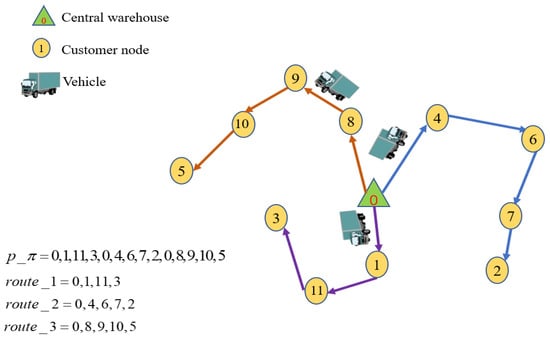
Figure 1. A sample solution for the 2L-OVRPTW.

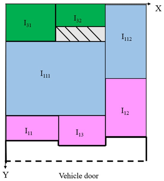
Figure 2. Loading scheme.

3.2. Mathematical Formulation

Goal: Minimize total travel distance and maximize customer satisfaction. The mathematical model of the 2L-OVRPTW is as follows:

$$min f_1={\displaystyle {\sum }_{k=1}^K{\displaystyle {\sum }_{i=0}^N{\displaystyle {\sum }_{j=0}^N{d}_{ij}{x}_{kij}}}}$$

(1)

$$max f_2=\frac{1}{N}{\displaystyle {\sum }_{i=1}^{N}ot{r}_i}$$

(2)

$${\displaystyle {\sum }_{i=0}^N{q}_i{y}_{ik}}\le Q , k\in K$$

(3)

$${\displaystyle {\sum }_{k=1}^K{y}_{ik}}=1 ,\forall i\in V^{\prime }$$

(4)

$${\displaystyle {\sum }_{j=1}^N{x}_{0jk}}=1,k\in K$$

(5)

$${\displaystyle {\sum }_{i=1}^N{x}_{i0k}}=0,k\in K$$

(6)

$${\displaystyle {\sum }_{i=0}^N{x}_{ijk}}=y_{jk},\forall j\in V^{\prime },k\in K$$

(7)

$${\displaystyle {\sum }_{j=0}^N{x}_{ijk}}=y_{ik},\forall i\in V^{\prime },k\in K$$

(8)

$$\begin{array}{c}0\le V_{kig}\le W-w_{kig},k\in K,\\ \forall i\in V^{\prime },\forall g\in M_i\end{array}$$

(9)

$$\begin{array}{c}0\le H_{kig}\le L-l_{kig} , k\in K,\\ \forall i\in V^{\prime },\forall g\in M_i\end{array}$$

(10)

$$\begin{array}{c}H{H}_{i{i}^{\prime }g{g}^{\prime }}=(\max (y_{ik}\cdot (H_{kig}+l_{ig}),y_{i^{\prime }{k}^{\prime }}\cdot (H_{k{i}^{\prime }{g}^{\prime }}+l_{i^{\prime }{g}^{\prime }}))\\ -\min (y_{ik}\cdot H_{kig},y_{i^{\prime }{k}^{\prime }}\cdot H_{k{i}^{\prime }{g}^{\prime }})-(y_{ik}\cdot l_{ig}+y_{i^{\prime }{k}^{\prime }}\cdot l_{i^{\prime }{g}^{\prime }})),\\ \forall i,i^{\prime }\in V^{\prime },\forall g,g^{\prime }\in M_i,\mathrm{g}\ne {\mathrm{g}}^{\prime },k,k^{\prime }\in K\end{array}$$

(11)

$$\begin{array}{c}L{L}_{i{i}^{\prime }g{g}^{\prime }}=(\max (y_{ik}\cdot (V_{kig}+w_{ig}),y_{i^{\prime }{k}^{\prime }}\cdot (V_{k{i}^{\prime }{g}^{\prime }}+w_{i^{\prime }{g}^{\prime }}))\\ -\min (y_{ik}\cdot V_{kig},y_{i^{\prime }{k}^{\prime }}\cdot V_{k{i}^{\prime }{g}^{\prime }})-(y_{ik}\cdot w_{ig}+y_{i^{\prime }{k}^{\prime }}\cdot w_{i^{\prime }{g}^{\prime }})),\\ \forall i,i^{\prime }\in V^{\prime },\forall g,g^{\prime }\in M_i,\mathrm{g}\ne \mathrm{g} \prime ,k,k^{\prime }\in K\end{array}$$

(12)

$$\max (H{H}_{i{i}^{\prime }g{g}^{\prime }},L{L}_{i{i}^{\prime }g{g}^{\prime }})\ge 0 , \forall i,i^{\prime }\in V^{\prime }, \forall g,g^{\prime }\in M_i$$

(13)

$$\begin{array}{c}\max (H{H}_{i{i}^{\prime }g{g}^{\prime }},(V_{kig}-V_{k{i}^{\prime }{g}^{\prime }}))\ge 0 , \\ \forall i,i^{\prime }\in V^{\prime }, \forall g,g^{\prime }\in M_i, i\ne i^{\prime }\end{array}$$

(14)

$$r{t}_j=s{t}_i+f_i+t_{ij},\forall i,j\in V^{\prime }$$

(15)

$$r{t}_j<h_j,\forall j\in V^{\prime }$$

(16)

$$s{t}_i=max(r{t}_i,e_i)$$

(17)

$$ot{r}_i\in \{0,1\}, i\in V^{\prime }$$

(18)

$$x_{ijk}\in \{0,1\},i,j\in V^{\prime },k\in K$$

(19)

$$y_{ik}\in \{0,1\},i\in V^{\prime },k\in K$$

(20)

In the above model, objective functions (1) and (2) give the objective functions of the 2L-OVRPTW, where function (1) represents the minimum total driving distance, and function (2) represents the maximum customer satisfaction. The constraints (3) ensure that the loading capacity does not exceed the maximum load capacity. Equation (4) ensures that all the customers can be served. Equations (5) and (6) indicate that all the vehicles should leave the central warehouse to serve a group of customers without returning to the central warehouse. Equations (7) and (8) ensure that each customer can only be served by one vehicle. Equations (9)–(14) are loading constraints. Equations (9) and (10) ensure that the loaded items do not exceed the scope of the carriage. Equations (11)–(13) ensure that the items do not overlap in the carriage. Equation (14) ensures that the items satisfy the first in and last out (FILO) principle. Equations (15)–(17) represent the time window constraints, where Equation (17) represents the possibility that the vehicle arrives early; if so, it needs to wait until the earliest service time. Equations (18)–(20) ensure the integrality constraints on the binary variable.

4. Solution Approach

The MLWOA proposed for the 2L-OVRPTW consists of two stages, the routing phase and the loading phase. The routing phase includes encoding and decoding, population initialization, the global search, and the local search. The loading phase load includes the scoring method, the arrangement of the loading sequence, and the disturbance mechanism. The general flow chart of the MLWOA is given at the end. For the convenience of expression, the symbols in this section and their definitions are given in Table 2.

Table 2. Symbols used in this section and their descriptions.

Symbol	Definition
$popsize$	The population size
$p\_\pi$	Individual integer sequence with central warehouse
$\pi$	Individual integer sequence without central warehouse
$X$	Real number location information corresponding to sequence $\pi$
$g$	The current iteration number
$Z$	The set including all unserved customers.
$ge{n}_{\max }$	The maximum iteration
${\pi }^g$	The population of generation $g$
${\pi }^{g,w}$	The individual $w$ in the population of generation $g$
$X^{g,w}$	Real number location information corresponding to individual $w$
$X^{g,w^{\prime }}$	A random individual in the population of generation $g$
$X^{g\ast }$	The non-dominant solution of generation $g$
${\pi }_{best}^{g,w}$	The non-dominated solution $w$ in the population of generation $g$
${\pi }_{best,p}^{g,w}$	The customer at the position $p$ in individual $w$ of generation $g$
${\pi }_i^{g,w}$	Customer $i$ in individual $w$ of generation $g$
$T{M}_{m\times n\times n}^g$	The three-dimensional information matrix, $n=N$, $m=N-1$
$T{M}_{m\times n\times n}^g(p)$	Two-dimensional block structure information matrix at position $p$
$T{M}_{m\times n\times n}^g(p,x,y)$	Elements in a three-dimensional information matrix
$P{M}_{m\times n\times n}^g$	Three-dimensional probability model based on a three-dimensional information matrix
$su{m}_p^g$	Represents the sum of all block structures at a position $p$ in generation $g$
$\cos \_sequence$	A collection of unserved customers
$tabu$	A collection of customers that have been serviced
$num\_best$	Represents the number of non-dominated solutions in the population

4.1. Encoding and Decoding

The important problem when applying the MLWOA to the 2L-OVRPTW involves finding a suitable mapping between the customer sequence and the individuals (continuous vectors) in the MLWOA. The 2L-OVRPTW is a discrete optimization problem; so, this paper adopts the largest order value (LOV) rule to map the real position information to the discrete position information. Similarly, after the discrete sequence changes, the real position information can also be adjusted by the reverse largest order value (RLOV) rule. The specific steps of the LOV rule are given below.

Step 1: $X^{g,w^{\prime }}$ is the sequence from the largest to the smallest, which can be obtained by real position information $X^{g,w}=[X^{g,w}[1],X^{g,w}[2],\dots ,X^{g,w}[g],\dots X^{g,w}[N]]$.

Step 2: Find out the corresponding position of each number in $X^{g,w^{\prime }}$ in $X^{g,w}$ and place it in ${\phi }^{g,w}$ in turn. Then, the intermediate sequence ${\phi }^{g,w}$ is obtained.

Step 3: Each number in the discrete sequence $P^{g,w}$ can be obtained by $P^{g,w}[{\phi }^{g,w}[g]]=g$.

As shown in Table 3, an example of the LOV rule is given. The individual sequence of real location information is $X^{g,w}=[1.49,2.41,2.17,1.78,2.06,1.80,0.88]$, and the sequence after ranking from the largest to the smallest is $X^{g,w^{\prime }}=[2.41,2.17,2.06,1.80,1.78,1.49,0.88]$. It can be seen that $X^{g,w}[1]=1.49$; so, the position is ${\phi }^{g,w}[1]=6$, $P^{g,w}[{\phi }^{g,w}[1]]=P^{g,w}[6]=1$, and with $X^{g,w}[2]=2.41$, the position is ${\phi }^{g,w}[2]=1$, $P^{g,w}[{\phi }^{g,w}[2]]=P^{g,w}[1]=2$. By analogy, the customer’s discrete sequence is $P^{g,w}=[2,3,5,6,4,1,7]$. After all the customers in $P^{g,w}$ are assigned a vehicle, the non-dominated solution must be an active schedule, in which the minimized total travel distance or maximized customer satisfaction is better than that of the other solutions.

Table 3. Example of LOV.

g	1	2	3	4	5	6	7
$X^{g,w}[g]$	1.49	2.41	2.17	1.78	2.06	1.80	0.88
${\phi }^{g,w}[g]$	6	1	2	5	3	4	7
$P^{g,w}[g]$	2	3	5	6	4	1	7

4.2. Population Initialization

The individual in the first generation of the population is generated by three rules. Firstly, Rule 1 and Rule 2 are used to generate two individuals, respectively; then, Rule 3 is used to generate other individuals. The detailed procedures of these rules are as follows:

Rule 1: Nearest principle

Let $i=0$, $j\in Z$, and $G=\varnothing$. The nearest customer $j$ can be funded by Equation (21). If $r{t}_j\in [e_j, h_j]$ are met, the customer $j$ will be served and moved from $Z$ to $G$. Let $i=j$ and find the next nearest customer to serve. Otherwise, let $i=0$ and choose another vehicle to service other customers.

$$min d_{ij}=\sqrt{{(x_i-x_j)}^2+{(y_i-y_j)}^2} , j\in Z$$

(21)

Rule 2: Satisfaction principle

Step 1: Let $i=0$, $j\in Z$, and $G=\varnothing$.

Step 2: Let $Z_0=\varnothing$. All the unserved customers that meet constraints (15)–(17) are placed in $Z_0$. Randomly select a customer $j$ in set $Z_0$ to service; if the constraints (3)–(14) are met, let $i=j$ and then move $j$ from $Z$ to $G$ and perform step 4. If no customer meets the constraints, then go to step 3.

Step 3: Select customer $j$ from $Z^{\prime }=Z\backslash \left\{Z_0\right\}$. If the constraints are met, let $i=j$ and move $j$ from $Z$ to $G$. If there are no customers that can meet the constraints, perform step 4.

Step 4: If $Z=\varnothing$, output $G$. Otherwise, return to step 1.

Rule 3: Quasi-opposition strategy

The quasi-opposition strategy refers to the opposite individual $j$ $X^{g,j}=[X^{g,j}[1],X^{g,j}[2],\dots ,X^{g,j}[g],\dots ,X^{g,j}[N]]$$(X^{g,j}[g]\in [a,b])$ of individual $i$ calculated by Equation (22) in the real field $[a,b]$.

$$X^{g,j}[g]=\{\begin{array}{l}rand\left(\overline{X},X^{g,i}[g]\right)X^{g,i}[g]>\overline{X}\\ rand\left(X^{g,i}[g],\overline{X}\right)X^{g,i}[g]\le \overline{X}\end{array} , \overline{X}=\frac{a+b}{2}$$

(22)

The initial population can be generated according to the three rules. And a non-dominated solution set is formed by the high-quality solutions in the population.

4.3. Global Search

Global search consists of exploitation mechanisms and a learning strategy. They are introduced in detail below. The symbols in this section and their definitions are given in Table 4.

Table 4. Symbols used in this section and their definitions.

Symbol	Definition
$r_1, r_2$	The random numbers in [0, 1]
$a_{int},a_{fin}$	The initial and terminal values, which are 0 and 2, respectively
$\mu$	The coefficient of the nonlinear adjustment
$b$	The parameter controlling the spiral shape
$l$	The random number in [0, 1]
$p_0$	The random number in [0, 1]

4.3.1. Exploration Mechanisms

In the WOA, the individual randomly selected from the non-dominated solution set is regarded as the prey, and the other individuals are whales. By simulating the process of a whale catching prey, the whale keeps approaching the prey position and guides the optimization algorithm, which includes three mechanisms that are used to search for the high-quality solution area.

$$D=\left|C{X}^{g\ast }-X^{g,w}\right|$$

(23)

$$a=a_{int}-a_{fin}+\raisebox{1ex}{$1-g/ge{n}_{\max }$}\!\left/ \!\raisebox{-1ex}{$1-\mu \cdot g/ge{n}_{\max }$}\right.$$

(24)

$$A=2a{r}_1-a$$

(25)

$$C=2r_2$$

(26)

Equation (23) indicates the absolute value of the distance between the individual $X^{g,w}$ and the non-dominant solution $X^{g\ast }$. Equation (24) shows the calculation process of nonlinear factor $a$ and the coefficient $\mu =25$. Equations (25) and (26) show the calculation process of the coefficients; $A$ and $C$ are the coefficients [31]. The mechanisms are expressed as follows:

Surrounding search mechanism: After determining the location of the non-dominant solution, the other individuals would keep approaching the prey. Equation (27) is used for the calculation of the surrounding search mechanism.

$$X^{g+1,w}=X^{g\ast }-A\cdot D$$

(27)

Spiral search mechanism: After calculating the distance between the non-dominant solution and individuals, the spiral Equation (28) is then created to mimic the helix-shaped movement.

$$X^{g+1,w}=D\cdot e^{b\cdot l}\cos (2\pi l)+X^{g\ast }$$

(28)

In Equation (29), the individual approaches the high-quality solution in the form of a reduced circle or along a spiral path. In order to simulate this simultaneous behavior, we assume that during the optimization process, $\gamma$ is the probability that the surrounding search mechanism or the spiral search mechanism is chosen to update the individual position.

$$X^{g+1,w}=\{\begin{array}{l}{X}^{g\ast }-A\cdot D,\hspace{1em}{p}_0<\gamma \\ D\cdot e^{b\cdot l}\cos (2\pi l)+X^{g\ast }, p_0\ge \gamma \end{array}$$

(29)

Random search mechanism: An individual that was randomly selected would be used to update the location of other individuals in the population. Equation (30) indicates the absolute value of the distance between the individual $X^{g,w}$ and a random individual $X^{g^{\prime }}$. Equation (31) is used for the calculation of the random search mechanism.

$$D^{\prime }=|C{X}^{g^{\prime }}-X^{g,w}|$$

(30)

$$X^{g+1,w}=X^{g^{\prime }}-A\cdot D^{\prime }$$

(31)

The WOA starts with an initialized population. In each iteration, the individuals update their location based on the randomly selected individual or the non-dominant solution that is currently obtained. When $\left|A\right|>1$, select the randomly individual $X^{g^{\prime }}$, and when $\left|A\right|\le 1$, select non-solution $X^{g\ast }$. According to the value of $p_0$, it can switch between the surrounding search mechanism and the spiral search mechanism. The mechanisms in WOA have the advantages of simple operation, the ability to find the optimal solution quickly, and good convergence and stability for various types of optimization problems.

4.3.2. Learning Strategy

After the global search with the WOA-based mechanisms, the next process in the MLWOA is the learning strategy. It includes the block structure, three-dimensional information matrix, and three-dimensional probability matrix, which are designed to accumulate each customer location and the order relationship information of the non-dominated solutions. The relevant definitions are as follows:

Block structure: This consists of two adjacent customers in any solution of the 2L-OVRPTW. Therefore, the number of the block structure in a solution is $n-1$ if there are $n$ customers in this solution. The customer service order information in the block structure is given by the Equation (32). If the block structure $[x, \mathrm{y}]$ exists, $ONE\_T_{p\times x\times y}^{g,w}=1$, otherwise, $ONE\_T_{p\times x\times y}^{g,w}=0$.

$$\begin{array}{c}ONE\_T_{p\times x\times y}^{g,w}=\{\begin{array}{l}1,if \mathrm{x}={\pi }_{best,P}^{g,w}, y=Best\_{\pi }_{best,p+1}^{g,w}\\ 0,else\end{array},\\ p=1,2,\cdots ,m \mathrm{x},\mathrm{y}=1,2,\cdots ,n\end{array}$$

(32)

Three-dimensional information matrix: An example is shown in Figure 3; the first dimension ($m$) records the location of the block structures. The two-dimensional matrix ($n,n$), which is composed of the second and third dimensions, records the information of the customer service order of all the block structures in the same location. The specific mathematical formulas of the three-dimensional information matrix description are as follows:

$$\begin{array}{c}T{M}_{m\times n\times n}^g(p,x,y)={\displaystyle {\sum }_{w=1}^{num\_best}ONE\_T_{m\times n\times n}^{g,w}(p,x,y)},\\ p=1,2,\cdots ,m \mathrm{x},\mathrm{y}=1,2,\cdots ,n\end{array}$$

(33)

$$\begin{array}{lll}T{M}_{m\times n\times n}^g(p)& =& [T{M}_{m\times n\times n}^g(p,x,1),\cdots ,T{M}_{m\times n\times n}^g(p,x,n)]\\ & =& \left[\begin{array}{ccc}T{M}_{m\times n\times n}^g(p,1,1), & \cdots , & T{M}_{m\times n\times n}^g(p,1,n)\\ ⋮& \ddots & ⋮\\ T{M}_{m\times n\times n}^g(p,n,1), & \cdots , & T{M}_{m\times n\times n}^g(p,n,n)\end{array}\right]\end{array}$$

(34)

$$\begin{array}{lll}T{M}_{m\times n\times n}^g& =& [T{M}_{m\times n\times n}^g(1),T{M}_{m\times n\times n}^g(2),\cdots ,\\ & & T{M}_{m\times n\times n}^g(p),\cdots ,T{M}_{m\times n\times n}^g(m)]\end{array}$$

(35)

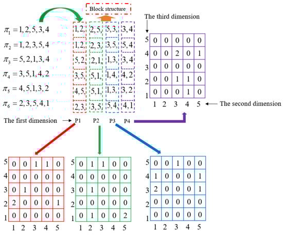
Figure 3. Three-dimensional information matrix.

Equations (33)–(35) give the hierarchical structure of the three-dimensional information matrix. Equation (33) is used to count the distribution information of all the block structures. $T{M}_{m\times n\times n}^g(p,x,y)$ represents the element which is the cumulative number of the block structure $[x, \mathrm{y}]$ at position $P$. The $T{M}_{m\times n\times n}^g(p)$ given in Equation (34) is a two-dimensional matrix ($n,n$) and refers to the customer service order information of all the block structures at location $P$. In Equation (35), the $T{M}_{m\times n\times n}^g$ is a three-dimensional information matrix; it records the information of all the block structures in the non-dominated solution set.

Three-dimensional probability matrix: After the three-dimensional information matrix is determined, the three-dimensional probability matrix will be calculated in the next step. The specific mathematical formulas are as follows:

$$su{m}_p^g={\displaystyle {\sum }_{x=1}^n{\displaystyle {\sum }_y^{n}T{M}_{m\times n\times n}^g(p,x,y), p=1,2,\cdots ,m }}$$

(36)

$$P{M}_{m\times n\times n}^g(p)=\left[\begin{array}{ccc}\frac{T{M}_{m\times n\times n}^g(p,1,1)}{su{m}_p^g}, & \cdots , & \frac{T{M}_{m\times n\times n}^g(p,1,n)}{su{m}_p^g}\\ ⋮& & ⋮\\ \frac{T{M}_{m\times n\times n}^g(p,n,1)}{su{m}_p^g}, & \cdots , & \frac{T{M}_{m\times n\times n}^g(p,n,n)}{su{m}_p^g}\end{array}\right]$$

(37)

$$\begin{array}{ccc}P{M}_{m\times n\times n}^g& =& [P{M}_{m\times n\times n}^g(1),P{M}_{m\times n\times n}^g(2),\cdots ,\\ & & P{M}_{m\times n\times n}^g(p),\cdots ,P{M}_{m\times n\times n}^g(m)]\end{array}$$

(38)

$$P{M}_{m\times n\times n}^{g+1}=\eta \cdot P{M}_{m\times n\times n}^{g+1}+(1-\eta )P{M}_{m\times n\times n}^g$$

(39)

In Equation (36), the $su{m}_p^g$ represents the number of all the block structures in position $P$. Equation (37) gives the probability of each element in $P{M}_{m\times n\times n}^g(p)$ at position P. Equation (38) gives the three-dimensional probability matrix. Equation (39) represents the update method of the probability matrix, and $\eta$ is the random numbers in $[0, 1]$.

As shown in Figure 3, an example of a three-dimensional information matrix that includes six individuals is given. For example, in the first individual, ${\pi }_1=[1,2,5,3,4]$, the block structures are [1, 2], [2, 5], [5, 3], and [3, 4]. In addition, at the position $P=1$, there are six block structures, including [1, 2], [1, 2], [5, 2], [3, 5], [4, 5], and [2, 3]. Therefore, in the three-dimensional information matrix, the values of the elements with subscripts the (1, 2, 3), (1, 3, 5), (1, 4, 5), and (1, 5, 2) are 1; the value of the element with the subscripts (1, 1, 2) is 2; and the other elements are 0.

As mentioned above, the new individuals can be generated based on the three-dimensional probability matrix. The pseudocode of the update strategy is shown in Algorithm 1.

The pseudocode of the update strategy is shown in Algorithm 1.

Algorithm 1 Update strategy
1:	Input:
2:	Set the number of $popsize$ and N.
3:	Begin:
4:	Set $loop=1$, $num=1$, $p=1$.
5:	while $loop\le \max \_l$ do
6:	Calculate the $T{M}_{m\times n\times n}^g$ through the non-dominated solution set ${\pi }_{best}^g$.
7:	while $num\le num\_bes{t}^g$ do
8:	while $p\le num\_customer$ do
9:	Generate the probability matrix of position $p$ as $P{M}_{m\times n\times n}^g(p)$.
	$sum={\displaystyle {\sum }_{x=1}^n{\displaystyle {\sum }_{y=1}^{n}P{M}_{m\times n\times n}^g(p,x,y)}}$
10:	if $sum>0$, then
11:	Place the block structure in the position $p$ and the $tabu$
12:	Let $p=p+2$.
13:	else
14:	Randomly select a customer from $co{s}_{-}sequence$ to position $p$ and the $tabu$
15:	Let $p=p+1$.
17:	end if
18:	end while
19:	Put the $tabu$ into the population as an individual
20	Let $num=num+1$
21:	end while
22:	Update the ${\pi }^g$ and ${\pi }_{best}^{\mathrm{g}}$
23:	Let $loop=loop+1$
24:	end while
25:	Output:
26:	The current population ${\pi }^g$ and its non-dominated solution set ${\pi }_{best}^g$

4.4. Local Search

After the global search, a better non-dominated solutions set is obtained. However, the 2L-OVRPTW has a large solution space, and the non-dominated solutions are distributed in various regions. Therefore, the local search of the MLWOA is used for the exploitation of the non-dominated solutions. As shown in Figure 4, Figure 5 and Figure 6, this section designs a local search with three neighborhood operations.

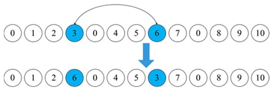
Figure 4. Interchange operation.

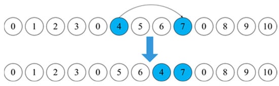
Figure 5. Insert operation.

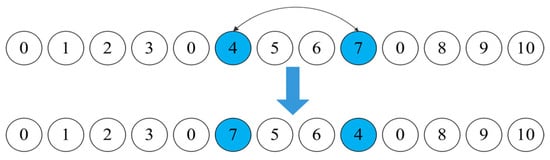
Figure 6. Swap operation.

Interchange operation: Randomly select customer $i$ and customer $j$ from $route[k]$ and $route[l]$, respectively, and then exchange them.

Insert operation: Randomly select two non-adjacent customers $i$ and customer $j$ in $route[k]$, and then insert the customer $i$ in front of customer $j$.

Swap operation: Randomly select customers $i$ and customer $j$ in $route[k]$, and then exchange them.

After each operation, if a better solution that satisfies the constraints is generated, the better solution will replace the current optimal solution. Otherwise, it will not be accepted.

The complexity analysis for the algorithm is detailed as follows. Let the population size of the MLWOA be $popsize$, the number of customers be $N$, the number of global search iterations be $ge{n}_{global}$, the number of updates based on the three-dimensional probability matrix be $max\_l$, the number of local search iterations be $ge{n}_{local}$, and the average total number of neighborhood operations used during the local search be $Z$. The algorithm complexity $T_{MLWOA}$ of the MLWOA consists of global search complexity and local search complexity. The algorithm complexity of the MLWOA consists of global search complexity and local search complexity, where the global search complexity includes the complexities of the initialization of the population $O(popsize\ast N)$, the updating of the three-dimensional probability matrix $O(popsize\ast 2\ast N^2)$, the generation of individuals based on the sampling probability matrices $O(popsize\ast N)$, and the evaluation of the population $O(popsize\ast N)$. The local search complexity is $O(ge{n}_{local}\ast Z\ast N)$. Therefore, $T_{MLWOA}=O(ge{n}_{global}\ast (max\_l\ast popsize\ast N^2+ge{n}_{local}\ast Z\ast N))$.

The pseudocode of the local search is shown in Algorithm 2.

Algorithm 2 Variable neighborhood local search
1:	Input:
2:	Set $max\_search=10$, $loop=1$, $N\_inter=1$, $N\_ins=1$, $N\_swap=1$ and $N\_max=10$.
3:	Begin:
4:	while $loop\le 10$ do
5:	while $N\_inter\le 10$. do
6:	Randomly select a solution ${\pi }_{best}^{g,w}$, randomly select vehicle $k$ and vehicle $l$,
	$k,l\in {\pi }_{best}^{g,w}$, and randomly select customer $i$ and customer $j$.$i\in vehicle k$,
	$j\in vehicle l$, then $int\_{\pi }_{best}^{g,w\ast }$=interchange$({\pi }_{best}^{g,w},k,l,i,j)$
7:	if $int\_{\pi }_{best}^{g,w\ast }$ satisfies all constraints, then
8:	${\pi }_{best}^{g,w}=int\_{\pi }_{best}^{g,w\ast }$
9:	else $N\_inter=N\_inter+1$
10:	end while
11:	while $N\_ins\le 10$ do
12:	Randomly select vehicle $k$, $k\in {\pi }_{best}^{g,w}$, randomly select customer $i$ and customer $j$,
	$i,j\in vehicle k$, then $ins\_{\pi }_{best}^{g,w\ast }$=insert$({\pi }_{best}^{g,w},k,i,j)$
15:	if $ins\_{\pi }_{best}^{g,w\ast }$ satisfies all constraints, then
16:	$ins\_{\pi }_{best}^{g,w}=ins\_{\pi }_{best}^{g,w\ast }$
19:	else $N\_ins=N\_ins+1$
20:	end while
21:	while $N\_swap\le 10$ do
22:	Randomly select vehicle $l$, $l\in {\pi }_{best}^{g,w}$, and randomly select customer $i$ and customer $j$,
	$i,j\in vehicle l$, then $swap\_{\pi }_{best}^{g,w\ast }$=swap$({\pi }_{best}^{g,w},l,i,j)$
23:	if $swap\_{\pi }_{best}^{g,w\ast }$ satisfies all constraints, then
24:	${\pi }_{best}^{g,w}=swap\_{\pi }_{best}^{g,w\ast }$
27:	else $N\_swap=N\_swap+1$
28:	end while
30:	$loop=loop+1$
31:	end while
32:	Output:
33:	Updated non-dominated solution set ${\pi }_{best}^g$.

4.5. Loading Strategy

The 2L-OVRPTW is integrated by the routing subproblem and the loading subproblem. The non-dominated solutions optimized by the MLWOA’s routing phase also need to be loaded. This section describes in detail how to optimize the loading process of the non-dominated solutions by the MLWOA’s loading phase.

The loading strategy based on the skyline mainly consists of a scoring method, the arrangement of the loading sequence, and the disturbance mechanism.

4.5.1. Loading Sequence

The loading sequence of the customers adopts the first in and last out (FILO) principle. For example, the service sequence of the route is [4,5,6,7]. It can be seen that the loading sequence is [7,6,5,4]. Obviously, the FILO principle can save service time.

In addition, the number of each customer’s items is not unique; Rule 4 and Rule 5 are used to initialize the order of each customer’s items. Then, all the items are loaded into the carriage through the scoring method.

Rule 4: Initialize and sort according to the length of the first customer’s items from small to large.

Rule 5: Initialize and sort according to the size of the rest of the customers’ items from small to large.

4.5.2. Scoring Method

The scoring method is an important part of the skyline-based loading strategy. As shown in Figure 7, the red line segment represents the horizontal skyline, and the green line segment represents the vertical skyline. The figure shows all the scores that would appear when an item I was placed on any horizontal skyline. That means that the items placed on each horizontal skyline receive a score, with a full score of 5 points.

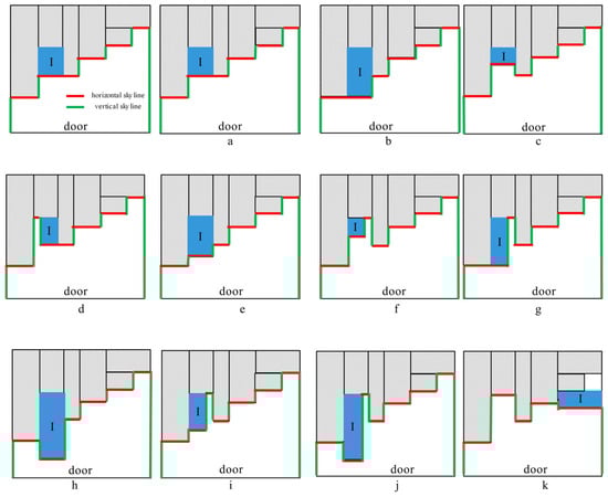
Figure 7. Scoring method. (a,b) Five points; (c,d) Four points; (e–g) Three points; (h–j) Two points; (k) One point.

The specific scoring methods are as follows:

Five points: When the width of the item is equal to the horizontal skyline of the current segment: if the length of the item is equal to the length of the vertical skyline on either side of the adjacent sides, the score is 5 points, as shown in parts (a) and (b).

Four points: There are two cases; the first is that the width of the item is equal to the horizontal skyline of the current segment, and the length is less than the vertical skyline on the adjacent two sides, as shown in part (c) in Figure 7. The other is that the width of the item is less than the horizontal skyline of the current segment, and the length is equal to the shorter side of the vertical skyline on both adjacent sides, as shown in part (d).

Three points: There are three cases; the first is that the width of the item is equal to the horizontal skyline of the current segment, and the length is between both adjacent sides, as shown in part (e) in Figure 7. The second is that the width is less than the horizontal skyline of the current segment, and the length is less than the vertical skyline on both adjacent sides, as shown in part (f) in Figure 7. Finally, the width is less than the horizontal skyline of the current segment, and the length is equal to the vertical skyline of the longer side on both adjacent sides, as shown in part (g).

Two points: There are three cases; the first is that the width of the item is equal to the horizontal skyline of the current segment, and the length is more than the vertical skyline on both adjacent sides, as shown in part (h) in Figure 7. The second is that the width is less than the horizontal skyline of the current segment, and the length is between the vertical skylines on both adjacent sides, as shown in part (i) in Figure 7. Finally, the width is less than the horizontal skyline of the current segment, and the length is more than the vertical skyline on both adjacent sides, as shown in part (j).

One point: If the width of the item is more than the horizontal skyline of the current segment, the score is 1 point, as shown in part (k).

If all horizontal skylines are less than the item’s width, the horizontal skylines that need to be filled are selected before loading the item. Otherwise, the item will be inserted at the horizontal skyline position with the highest score, and the skyline will be updated. As shown in Figure 8, the loading process of the customer’s items is given. The solid line represents the customer’s service sequence, and the dotted line represents the customer’s item loading sequence.

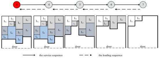
Figure 8. Distribution route and skyline update.

4.5.3. Disturbance Mechanism

Integrating a disturbance mechanism is conducive to the optimization of the loading processes. If the loading process is unreasonable, there may be a large area of redundant space, which will make it impossible to load all the customers’ items on the service route into the carriage. In view of this situation, the loading order of two items of any customer are randomly selected to exchange and are then re-loaded, as shown in parts (a) and (b) in Figure 9.

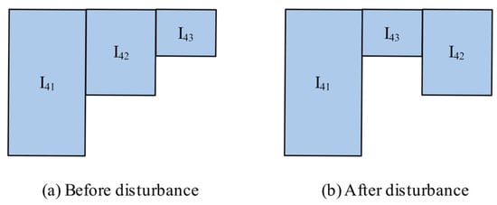
Figure 9. Exchanging the loading sequence of items.

Table 5 below shows the comparison results of the loading success rate related to whether or not the disturbance mechanism is used in the different customer sizes. The No represents the non-use of the disturbance mechanism, and the Yes represents the use of the disturbance mechanism during loading. Among them, the success rate refers to the proportion of the number of times that all the goods are loaded into the carriage after 20 independent operations. It can be clearly seen that the results after adding the disturbance mechanism are significantly higher. In Figure 10, the flow chart of the MLWOA, except for loading, and the flow chart of loading can be seen.

Table 5. Loading success rate.

Customer Size	Instances	Success Rate
		No	Yes
15	2l_cvrp103	0.75	0.90
20	2l_cvrp403	0.65	0.80
21	2l_cvrp603	0.60	0.90
25	2l_cvrp903	0.55	0.85
30	2l_cvrp1203	0.90	0.90
35	2l_cvrp1603	0.50	0.80
40	2l_cvrp1703	0.80	0.90
44	2l_cvrp1803	0.70	0.85
50	2l_cvrp1903	0.55	0.75
75	2l_cvrp2403	0.35	0.80
100	2l_cvrp2703	0.40	0.75
120	2l_cvrp2803	0.35	0.55
199	2l_cvrp3103	0.35	0.65

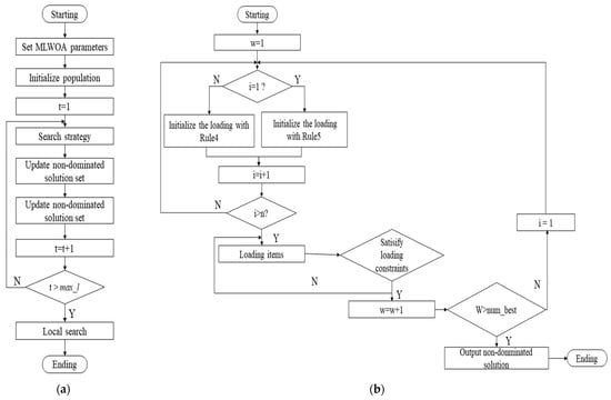
Figure 10. (a) Flow chart of MLWOA except loading; (b) flow chart of loading.

The pseudocode of the MLWOA algorithm is shown in Algorithm 3.

Algorithm 3 Multi-objective learning whale optimization algorithm
1:	Input:
2:	Set $gen\_\max$, $popsize$, $\max \_l$, $\gamma$
3:	Begin:
4:	Let $l\in random[-1,1],$$p\in random[0,1]$
5:	Population initialization
6:	while $g\le gen\_\max$ do
7:	while $t\le \max \_l$ do
8:	while $i<popsize$ do
9:	if $A\le 1$, then
10:	Update ${\pi }^{g,i}$ by Equation (30)
11:	else
12:	if $p<\gamma$, then
13:	Update ${\pi }^{g,i}$ by Equation (24)
14:	else
15:	Update ${\pi }^{g,i}$ by Equation (27)
16:	end if
17:	end if
18:	$i=i+1$
19:	end while
20:	$t=t+1$
21:	end while
22:	Update the population, non-dominated solution set and three-dimensional probability matrix
23:	for ${\pi }_{best}^{g,w}\in {\pi }_{best}^g$, do
24:	Initialize the loading sequence of all items of customers by Rule 4 and Rule 5.
25:	for $M{M}_{i,k}\in {\pi }_{best}^{g,w}$ do
26:	for $c\in M{M}_{i,k}$ do
27:	for $I_{ng}\in c$ do
28:	Loading the customer’s items into the carriage by the loading strategy.
29:	end for
30:	end for
31:	end for
32:	end for
33:	$g=g+1$
34	end while
35:	Output:
36:	Return the non-dominated solution set ${\pi }_{best}^g$.

5. Simulation Experiment and Comparative Analysis

5.1. Experimental Setup

As there is currently no dataset suitable for 2L-OVRPTW, this paper selects an available international dataset related to VRP (datasets from http://www.bernabe.dorronsoro.es/vrp/ (accessed on 1 January 2024)). All experiments are run on Windows 10 platform, which has 3.0 GHz CPU and 16 GB RAM, and are on a single thread. The algorithms in this paper are implemented by Python 3.7. The coordinates of the central warehouse and its service time window are (0, 0) and $[0, \infty ]$, respectively. Each vehicle’s load capacity $Q$ is 200. The items in the datasets are generated by using the method from references [30,32], as shown in Table 6. In this paper, there are datasets of different customer sizes. There are four categories, as shown in Table 6. Category 4 is used to generate all items in an instance containing 25 customers, and the items of the other instances are randomly generated by the other categories. Each category can randomly generate the number $M_i$ of items required by the customer $i$. Vertical, uniform, and horizontal are three different ways to generate the shape of all the items. The length and width of each item are generated based on the (L, W) of the carriage. The L and the W refer to the length and width of the carriage, respectively, and their values are (40, 20).

Table 6. Rectangular corresponding items.

Category	${\mathit{M}}_{\mathit{i}}$	Vertical		Uniform		Horizontal
		Length	Width	Length	Width	Length	Width
1	[1, 2]	[0.4 L, 0.9 L]	[0.1 W, 0.2 W]	[0.2 L, 0.5 L]	[0.2 W, 0.5 W]	[0.1 L, 0.2 L]	[0.4 W, 0.9 W]
2	[1, 3]	[0.3 L, 0.8 L]	[0.1 W, 0.2 W]	[0.2 L, 0.4 L]	[0.2 W, 0.4 W]	[0.1 L, 0.2 L]	[0.3 W, 0.8 W]
3	[1, 4]	[0.2 L, 0.7 L]	[0.1 W, 0.2 W]	[0.1 L, 0.4 L]	[0.1 W, 0.4 W]	[0.1 L, 0.2 L]	[0.2 W, 0.7 W]
4	[1, 5]	[0.1 L, 0.6 L]	[0.1 W, 0.2 W]	[0.1 L, 0.3 L]	[0.1 W, 0.3 W]	[0.1 L, 0.2 L]	[0.1 W, 0.6 W]

5.2. Performance Index and Parameter Setting

5.2.1. Performance Index

(1)

$N$ index

For the non-dominated solution sets obtained by the different algorithms, the more non-dominated solutions in the set, the better the algorithm’s performance in solving the problem.

(2)

$\overline{N}$ index

This performance is evaluated by counting the number of solutions remaining after the set of non-dominated solutions obtained by the algorithm is dominated by the other non-dominated solutions.

$$N(S_j)=\left|S_j-\{x\in S_j|\exists y\in S_{sum}:y\prec x\}\right|$$

(40)

In Formula (40), $S_{sum}$ represents the set of non-dominated solutions obtained by all the algorithms, and $S_j$ is the solution set of the non-dominated solutions found by algorithm $j$. $N(S_j)$ represents the number of solutions remaining after the other non-dominated solution sets dominate the non-dominated solution set obtained by the algorithm $j$.

(3)

$R$ index

In Formula (41), $R(S_j)$ represents the ratio of the solution obtained by the algorithm $j$ in $S_{sum}$ to the non-dominated solution set obtained by algorithm $j$

$$R(S_j)=\left|S_j-\{x\in S_j|\exists y\in S_{sum}:y\prec x\}\right|/\left|S_j\right|$$

(41)

5.2.2. Parameter Setting

The parameters involved in the MLWOA include the population size, the search factor, and the number of iterations based on the three-dimensional probability matrix; these are denoted by by $popsize$, $\gamma$, and $max\_l$, respectively. This paper selects the C201 instance for parameter testing and analysis in the dataset. The DOE method is used to discuss the influence of each parameter on the performance of the MLWOA. First, four level values are set for each parameter, then an L16 (4³) orthogonal test table is established. As shown in Table 7, Table 8 and Table 9, The first target value is the average value of the number of non-dominated solutions divided by the population size after each group of parameters runs 20 times. The sum of all the non-dominated solutions obtained by running 20 times is denoted by $S\_P$. $S\_R$ is the number remaining after removing the dominated solution from $S\_P$; so, the second target value is $\raisebox{1ex}{$S\_R$}\!\left/ \!\raisebox{-1ex}{$S\_P$}\right.$. The target values are each worth 50% in RV, which is used as an evaluation metric to analyze the parameter performance.

Table 7. Parameter level.

Parameter	Level
	1	2	3	4
$popsize$	30	50	70	90
$\gamma$	0.2	0.4	0.6	0.8
$max\_l$	20	40	60	80

Table 8. Orthogonal test results.

Parameter Combination Number	Parameter Level			RV
	$\mathit{p}\mathit{o}\mathit{p}\mathit{s}\mathit{i}\mathit{z}\mathit{e}$	$\mathit{\gamma }$	$\mathit{m}\mathit{a}\mathit{x}\_\mathit{l}$
1	1	4	3	0.628
2	1	3	4	0.628
3	1	2	2	0.612
4	1	1	1	0.612
5	2	4	1	0.626
6	2	3	2	0.643
7	2	2	4	0.653
8	2	1	3	0.648
9	3	4	1	0.653
10	3	3	3	0.658
11	3	2	2	0.651
12	3	1	4	0.653
13	4	4	3	0.673
14	4	3	2	0.678
15	4	2	1	0.653
16	4	1	4	0.679

Table 9. Average response value of parameters.

Level	Parameters
	$\mathit{p}\mathit{o}\mathit{p}\mathit{s}\mathit{i}\mathit{z}\mathit{e}$	$\mathit{\gamma }$	$\mathit{m}\mathit{a}\mathit{x}\_\mathit{l}$
1	0.620	0.648	0.636
2	0.642	0.642	0.646
3	0.660	0.658	0.658
4	0.671	0.645	0.653
range	0.051	0.016	0.022
grade	1	3	2

Therefore, the parameter combination set based on the experimental analysis is $popsize=70$, $\gamma =0.6$, $max\_l=60$.

5.3. Comparison with Standard WOA

To verify the effectiveness of the MLWOA, the MLWOA was compared with the WOA. Several instances, including 25, 50, and 100 customers, were selected for experimental analysis. The experimental results after running for the same time are shown in Table 10. The optimal results are shown in bold. The performance of the Wilcoxon rank-sum test based on the $N$, $\overline{N}$, and $R$ parameters is shown in Table 10. Table 11 shows that with p < 0.001, the effectiveness of the MLWOA algorithm is significantly higher than that of the WOA algorithm.

Table 10. Comparison results of the MLWOA with WOA.

Customer Size	Instances	WOA			MLWOA
		$\mathit{N}$	$\overline{\mathit{N}}$	$\mathit{R}$	$\mathit{N}$	$\overline{\mathit{N}}$	$\mathit{R}$
25	C101	17	1	0.059	31	19	0.613
	C102	12	1	0.083	35	18	0.514
	C103	10	6	0.600	21	11	0.524
	C104	11	2	0.182	30	17	0.567
	C105	14	1	0.071	31	12	0.387
	C106	25	2	0.080	32	18	0.563
	C107	18	3	0.167	41	6	0.146
	C108	13	1	0.077	29	21	0.724
	C109	14	1	0.071	37	19	0.514
	C201	19	1	0.053	30	10	0.333
50	C101	12	0	0.000	29	29	1.000
	C102	15	4	0.267	18	8	0.444
	C103	2	2	1.000	22	12	0.545
	C104	12	3	0.250	39	17	0.436
	C105	8	1	0.125	41	16	0.390
	C106	22	1	0.455	28	10	0.357
	C107	14	0	0.000	24	24	1.000
	C108	18	1	0.056	34	17	0.500
	C109	8	1	0.125	25	9	0.360
	C201	7	0	0.000	27	27	1.000
100	C101	10	1	0.100	24	18	0.750
	C102	8	0	0.125	27	27	1.000
	C103	13	1	0.077	37	33	0.892
	C104	12	2	0.167	25	14	0.560
	C105	12	1	0.083	26	19	0.731
	C106	8	0	0.000	26	26	1.000
	C107	12	1	0.083	27	21	0.778
	C108	16	1	0.063	36	31	0.861
	C109	15	1	0.067	31	18	0.581
	C201	15	2	0.133	31	21	0.677

Table 11. The results of the Wilcoxon rank-sum test for MLWOA and WOA.

Group	Median (P25, P75)	Wilcoxon Rank-Sum Test
		Z	p
$WOA\_N$	12.5 (10, 15.25)	−4.786	<0.001
$MLWOA\_N$	29.5 (25.75, 34.25)
$WOA\_\overline{N}$	1 (1, 2)	−4.784	<0.001
$MLWOA\_\overline{N}$	18 (12, 21.75)
$WOA\_R$	0.083 (0.062, 0.167)	−4.351	<0.001
$WOA\_R$	0.565 (0.442, 0.7988)

The MLWOA makes the search scope in the solution space wider and the search degree deeper and more detailed. The use of nonlinear factors in the MLWOA also makes the algorithm not fall into local optimization. Therefore, compared with the WOA, the number of non-dominant solutions obtained by the MLWOA is higher. In addition, the non-dominated solutions obtained by the two algorithms are liberated together. After removing the dominated solutions, the number of solutions from the MLWOA is obviously more than that of the WOA. This shows that the quality of the solutions obtained by the MLWOA is better.

5.4. Comparison with Other Algorithms

In order to verify the effectiveness of the MLWOA in solving the 2L-OVRPTW, this paper compares the MLWOA with other algorithms that solved similar problems at home and abroad, including the QPSO algorithm [21], VNS algorithm [18], and SAHLS algorithm [19]. The instances with 25, 50, and 100 customers are selected for testing. The results are shown in Table 12. For index $N$, all four algorithms can obtain some non-dominated solutions, but obviously, the number of non-dominated solutions obtained by the MLWOA is more. For index $\overline{N}$, after being dominated by the non-dominated solution sets of the other algorithms, all three algorithms (QPSO, VNS, and SAHLS) have a small number of non-dominated solutions left, while the MLWOA can retain most of the solutions. For index $R$, good results are achieved in the MLWOA. According to the results from Figure 11, it can be observed that our algorithm outperforms the other heuristic algorithms. For large-scale instances in particular, the MLWOA obtained more non-dominated solutions. The findings given above show that the MLWOA can effectively solve the 2L-OVRPTW.

Table 12. Comparison results of MLWOA with QPSO, VNS, and SAHLS.

Customer Size	Instances	QPSO			VNS			SAHLS			MLWOA
		$\mathit{N}$	$\overline{\mathit{N}}$	$\mathit{R}$	$\mathit{N}$	$\overline{\mathit{N}}$	$\mathit{R}$	$\mathit{N}$	$\overline{\mathit{N}}$	$\mathit{R}$	$\mathit{N}$	$\overline{\mathit{N}}$	$\mathit{R}$
25	C101	21	1	0.048	23	0	0.000	30	0	0.000	53	20	0.377
	C102	22	0	0.000	8	4	0.500	12	3	0.250	41	17	0.415
	C103	12	0	0.000	23	0	0.000	19	2	0.105	35	13	0.371
	C104	14	0	0.000	15	1	0.067	7	0	0.000	41	19	0.463
	C105	13	0	0.000	20	1	0.050	20	0	0.000	35	18	0.514
	C106	23	0	0.000	27	3	0.111	16	2	0.125	38	18	0.474
	C107	15	2	0.133	10	4	0.400	25	0	0.000	50	16	0.320
	C108	10	0	0.000	7	0	0.000	12	0	0.000	51	27	0.529
	C109	13	1	0.077	14	0	0.000	8	0	0.000	53	15	0.283
	C201	10	0	0.000	15	3	0.200	12	0	0.000	34	20	0.588
50	C101	15	1	0.067	14	0	0.000	12	1	0.083	60	23	0.383
	C102	11	0	0.000	13	0	0.000	17	1	0.059	43	24	0.558
	C103	9	0	0.000	14	3	0.214	21	0	0.000	49	21	0.429
	C104	10	1	0.100	11	1	0.091	22	0	0.000	51	25	0.490
	C105	19	0	0.000	7	3	0.428	13	0	0.000	59	19	0.322
	C106	13	0	0.000	18	1	0.056	23	0	0.000	52	27	0.519
	C107	17	2	0.117	11	0	0.000	15	0	0.000	50	41	0.820
	C108	13	0	0.000	12	1	0.083	13	0	0.000	61	22	0.361
	C109	15	0	0.000	16	1	0.062	21	0	0.000	62	22	0.355
	C201	11	0	0.000	15	0	0.000	14	1	0.071	38	16	0.421
100	C101	11	0	0.000	16	2	0.125	17	0	0.000	50	31	0.620
	C102	15	1	0.067	24	4	0.167	17	0	0.000	48	41	0.854
	C103	21	0	0.000	16	0	0.000	13	1	0.077	56	46	0.821
	C104	17	0	0.000	15	1	0.067	11	0	0.000	64	60	0.938
	C105	12	2	0.167	14	0	0.000	14	0	0.000	61	39	0.639
	C106	14	0	0.000	16	2	0.125	7	0	0.000	63	37	0.587
	C107	25	0	0.000	4	1	0.250	16	0	0.000	49	36	0.735
	C108	12	0	0.000	14	1	0.071	14	1	0.071	48	40	0.833
	C109	7	1	0.143	20	2	0.100	17	0	0.000	66	52	0.788
	C201	14	1	0.071	10	1	0.100	19	2	0.105	48	42	0.875

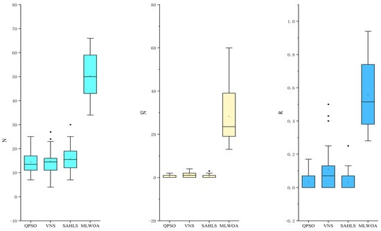
Figure 11. Box plots of results for 3 heuristics and MLWOA for different indexes.

The main reason is that the three-dimensional probability matrix used in the MLWOA’s learning strategy can not only learn valuable information about the customer order existing in the non-dominated solution but also accurately and reasonably record the position of each block structure. With the algorithm that only considers the order of customers, it is difficult to achieve the effect of the MLWOA. According to the above experiments and analysis, it can be concluded that the three-dimensional probability matrix plays an important role in the MLWOA.

6. Conclusions

In this paper, a learning whale optimization algorithm (MLWOA) is proposed to solve the two-dimensional loading open vehicle routing problem with time window constraints (2L-OVRPTW). The objective of the optimization is to minimize the distance and maximize customer satisfaction. The 2L-OVRPTW problem integrates both routing and loading problems. In this context, both problems need to be considered together. When solving this problem using the MLWOA, the individuals are first discretized using the LOV rules, allowing the population to be updated using the update mechanism of the whale optimization algorithm (WOA). During the initialization stage, diverse initial populations are generated using different rules. To better capture customer location and order relationship information in high-quality solutions, a three-dimensional probability matrix based on the block structure of adjacent customers is constructed. A loading strategy based on the skyline and scoring method is adopted to improve the loading efficiency. Compared to the standard WOA and the other algorithms in the literature, the computational results derived from the 2L-OVRPTW instances show that the MLWOA obtains better results than the others.

The future research will consider expanding two-dimensional loading to three-dimensional loading problems based on open vehicle routing problems and will consider more practical delivery constraints, such as pickup and delivery constraints, periodic constraints, etc. In terms of solution methods, different learning mechanisms will be integrated on the basis of the WOA, so that it can be applied in different scenarios.

References

- Dantzig, G.B.; Ramser, J.H. The Truck Dispatching Problem. Manag. Sci. 1959, 6, 80–91. [Google Scholar] [CrossRef]
- Letchford, A.N.; Lysgaard, J.; Eglese, R.W. A branch-and-cut algorithm for the capacitated open vehicle routing problem. J. Oper. Res. Soc. 2017, 58, 1642–1651. [Google Scholar] [CrossRef]
- Yu, N.K.; Qian, B.; Hu, R.; Chen, Y.W.; Wang, L. Solving open vehicle problem with time window by hybrid column generation algorithm. J. Syst. Eng. Electron. 2022, 33, 997–1009. [Google Scholar] [CrossRef]
- Zhao, F.; Zhang, L.; Cao, J.; Tang, J. A Cooperative Water Wave Optimization Algorithm with Reinforcement Learning for the Distributed Assembly No-idle Flowshop Scheduling Problem. Comput. Ind. Eng. 2020, 153, 107082. [Google Scholar] [CrossRef]
- Zhou, S.; Xing, L.; Zheng, X.; Du, N.; Wang, L.; Zhang, Q. A Self-Adaptive Differential Evolution Algorithm for Scheduling a Single Batch-Processing Machine with Arbitrary Job Sizes and Release Times. IEEE Trans. Cybern. 2021, 51, 1430–1442. [Google Scholar] [CrossRef] [PubMed]
- Cai, Y.; Cheng, M.; Zhou, Y.; Liu, P.; Guo, J.M. A hybrid evolutionary multitask algorithm for the multiobjective vehicle routing problem with time windows. Inf. Sci. 2022, 612, 168–187. [Google Scholar] [CrossRef]
- Michel, D.; Andrea, D.; Jean, D. Tabu search for the time-dependent vehicle routing problem with time windows on a road network. Eur. J. Oper. Res. 2021, 288, 129–140. [Google Scholar] [CrossRef]
- Marinakis, Y.; Marinaki, M.; Migdalas, A. A multi-adaptive particle swarm optimization for the vehicle routing problem with time windows. Inf. Sci. 2019, 481, 311–329. [Google Scholar] [CrossRef]
- Moradi, B. The new optimization algorithm for the vehicle routing problem with time windows using multi-objective discrete learnable evolution model. Soft Comput. 2020, 24, 6741–6769. [Google Scholar] [CrossRef]
- Shi, Y.; Zhou, Y.; Boudouh, T.; Grunder, O. A lexicographic-based two-stage algorithm for vehicle routing problem with simultaneous pickup–delivery and time window. Eng. Appl. Artif. Intell. 2020, 95, 103901. [Google Scholar] [CrossRef]
- Zhou, Y.; Kong, L.; Cai, Y.; Wu, Z.; Liu, S.; Hong, J.; Wu, K. A decomposition-based local search for large-scale many-objective vehicle routing problems with simultaneous delivery and pickup and time windows. IEEE Syst. J. 2020, 14, 5253–5264. [Google Scholar] [CrossRef]
- Barth, M.; Boriboonsomsin, K. Real-World Carbon Dioxide Impacts of Traffic Congestion. Transp. Res. Rec. J. Transp. Res. Board 2008, 2058, 163–171. [Google Scholar] [CrossRef]
- Xiao, Y.; Zuo, X.; Huang, J.; Konak, A.; Xu, Y. The continuous pollution routing problem. Appl. Math. Comput. 2020, 387, 125072. [Google Scholar] [CrossRef]
- Zhang, C.B.; Wang, W.Z.; Zhao, X.S.; Gu, J.W.; Yan, Y.Z. A Memetic Algorithm Based on Two_Arch2 for Multi-depot Heterogeneous-vehicle Capacitated Arc Routing Problem. Swarm Evol. Comput. 2021, 63, 100864. [Google Scholar] [CrossRef]
- Xiao, Y.; Zhang, Y.; Kaku, I.; Kang, R.; Pan, X. Electric vehicle routing problem: A systematic review and a new comprehensive model with nonlinear energy recharging and consumption. Renew. Sustain. Energy Rev. 2021, 151, 111567. [Google Scholar] [CrossRef]
- Iori, M.; José, J.; González, S.; Vigo, D. An Exact Approach for the Vehicle Routing Problem with Two-Dimensional Loading Constraints. Transp. Sci. 2007, 41, 253–264. [Google Scholar] [CrossRef]
- Fuellerer, G.; Doerner, K.F.; Hartl, R.F.; Iori, M. Ant colony optimization for the two-dimensional loading vehicle routing problem. Comput. Oper. Res. 2009, 36, 655–673. [Google Scholar] [CrossRef]
- Wei, L.; Zhang, Z.; Zhang, D.; Lim, A. A variable neighborhood search for the capacitated vehicle routing problem with two-dimensional loading constraints. Eur. J. Oper. Res. 2015, 243, 798–814. [Google Scholar] [CrossRef]
- Wei, L.; Zhang, Z.; Zhang, D.; Leung, S.C.H. A simulated annealing algorithm for the capacitated vehicle routing problem with two-dimensional loading constraints. Eur. J. Oper. Res. 2018, 265, 843–859. [Google Scholar] [CrossRef]
- Wang, Z.C.; Zhou, L. Modeling and Optimization of Vehicle Scheduling Problem with Two-dimensional Loading Constraints. Comput. Technol. Dev. 2018, 28, 105–110. [Google Scholar]
- Yan, R.; Zhu, X.N.; Zhang, Q.; Qi, Y.Y.; Lin, Y.Z. Research on model and algorithm of multi depot vehicle routing problem with time windows considering two-dimensional packing constraints. China Manag. Sci. 2017, 25, 67–77. [Google Scholar]
- Leung, C.H.; Stephen, Z.; Zhang, D.; Zhang, X.; Lim, M.K. A meta-heuristic algorithm for heterogeneous fleet vehicle routing problems with two-dimensional loading constraints. Eur. J. Oper. Res. 2013, 225, 199–210. [Google Scholar] [CrossRef]
- Sabar, N.R.; Bhaskarh, A.; Chung, E.; Turky, A.; Song, A. An Adaptive Memetic Approach for Heterogeneous Vehicle Routing Problems with two-dimensional loading constraints. Swarm Evol. Comput. 2020, 58, 100730. [Google Scholar] [CrossRef]
- Liu, W.; Zhou, Y.; Qiu, J.; Xie, N.; Chang, X.; Chen, J. A hybrid ACS-VTM algorithm for the vehicle routing problem with simultaneous delivery & pickup and real-time traffic condition. Comput. Ind. Eng. 2021, 162, 107747. [Google Scholar] [CrossRef]
- Seyedali, M.; Lewis, A. The Whale Optimization Algorithm. Adv. Eng. Softw. 2016, 95, 51–67. [Google Scholar] [CrossRef]
- Zheng, W.D.; Li, Z.G.; Jia, H.Z.; Gao, C. Study on prediction model of steel making end point based on improved whale optimization algorithm and least square support vector machine. J. Electron. 2019, 47, 700–706. [Google Scholar]
- Wang, T.; Xin, Z.; Miao, H.; Zhang, H.; Du, Y. Optimal Trajectory Planning of Grinding Robot Based on Improved Whale Optimization Algorithm. Math. Probl. Eng. 2020, 2020, 1–8. [Google Scholar] [CrossRef]
- Zeng, N.; Song, D.; Li, H.; You, Y.; Alsaadi, F.E. A Competitive Mechanism Integrated Multi-objective Whale Optimization Algorithm with Differential Evolution. Neurocomputing 2020, 432, 170–182. [Google Scholar] [CrossRef]
- Dewi, S.K.; Utama, D.M. A New Hybrid Whale Optimization Algorithm for Green Vehicle Routing Problem. Syst. Sci. Control Eng. 2021, 9, 61–72. [Google Scholar] [CrossRef]
- Yu, N.K.; Jiang, W.; Qian, B.; Hu, R.; Wang, L. Learning Whale Optimization Algorithm for Open Vehicle Routing Problem with Loading Constraints. Discret. Dyn. Nat. Soc. 2021, 2021, 1–14. [Google Scholar] [CrossRef]
- Long, W.; Cai, S.; Jiao, J.; Tang, M.; Tiebin, W.U. Improved whale optimization algorithm for solving large-scale optimization problems. Syst. Eng. Theory Pract. 2017, 37, 2983–2994. [Google Scholar]
- Gendreau, M.; Iori, M.; Laporte, G.; Martello, S. A Tabu Search Heuristic for The Vehicle Routing Problem With Two-Dimensional Loading Constraints. Networks 2008, 51, 4–18. [Google Scholar] [CrossRef]
Disclaimer/Publisher’s Note: The statements, opinions and data contained in all publications are solely those of the individual author(s) and contributor(s) and not of MDPI and/or the editor(s). MDPI and/or the editor(s) disclaim responsibility for any injury to people or property resulting from any ideas, methods, instructions or products referred to in the content. |
© 2024 by the authors. Licensee MDPI, Basel, Switzerland. This article is an open access article distributed under the terms and conditions of the Creative Commons Attribution (CC BY) license (https://creativecommons.org/licenses/by/4.0/).