Model Based Optimization of Energy Consumption in Milk Evaporators

Abstract

This work explores five falling film evaporator (FFE) simulation approaches combined with energy consumption minimization strategies, namely Mechanical Vapor Recompression and Thermal Vapor Recompression (MVR and TVR, respectively). Global system analysis and advanced dynamic optimization strategies are then investigated to minimize steam consumption, the cost of steam, and the total annualized cost and to maximize product yield. The results indicate that higher TVR discharge pressures, or MVR compression ratios, along with higher feed temperatures, enhance evaporation but increase operational costs. The most economical option includes three evaporator effects with TVR to achieve 50% product dry mass content. However, for a 35% dry mass content, MVR becomes cost-effective with an 11% reduction in unit electricity prices or a simultaneous 7% drop in electricity prices and a 5% increase in gas-based steam prices. Furthermore, switching from milk powder production to milk concentrates leads to an annual cost reduction ranging from 10.8 to 44%. Additionally, a forecasted 20% (or more) reduction in biomass-based steam cost can lead to lower annual expenditure compared with the nominal NG-based steam case. Regarding the total annualized cost, for a new plant design, optimization strategies lead to a 9–45% reduction in the total cost depending on the case under consideration.

1. Introduction

Evaporation involves the conversion of a solvent into vapor, which is then removed from a solution or slurry. In most cases, water is the solvent used in evaporation systems. This process entails vaporizing a portion of the solvent to create a concentrated solution, thick liquor, or slurry [1]. Dairy manufacturers commonly employ concentration techniques to produce dairy products with higher levels of dry matter, increased value, reduced volume, and extended shelf-life [2]. Lowering the water activity and reducing transportation and storage costs are key benefits of dehydrating dairy products. This process involves converting a liquid product into a dry powder by removing nearly all the available water. However, dairy products are sensitive to heat, and their functional properties and digestibility can be negatively affected by excessive heat during the dehydration process. Therefore, a single water removal method cannot consistently achieve optimal performance. It, thus, becomes necessary to employ multiple processing steps tailored to the specific properties of the material being processed while considering both product quality and processing costs [3].

Typically, the main steps involved in the production of milk powder include standardization, homogenization, pasteurization, evaporation, and drying [4]. Evaporation is a significant step in milk-powder production plants, serving not only to concentrate milk to the desired viscosity for subsequent spray drying but also to reduce the energy requirements during the spray drying process. In the evaporation stage, sterilized milk is concentrated under vacuum conditions at temperatures ranging from 40 to 70 °C. This process leads to a significant increase in the total solids content, which typically rises from around 13 to 50% [5]. Vacuum conditions are used to mitigate the negative effects of heat on heat-sensitive milk components like fats and to prevent the degradation of essential nutrients, such as vitamins.

Milk powder production consists of many thermal processes, including evaporation and drying, and is responsible for 15% of the total energy use in the dairy industry [4To this end, numerous energy-saving technologies have been applied in the milk evaporation process. The ones that are thoroughly examined in this work are the most commonly applied in industrial practice, namely (i) Mechanical Vapor Recompression (MVR) and (ii) Thermal Vapor Recompression (TVR) technologies.

• In the evaporator unit, the excess heat generated by the secondary steam is typically released as waste heat. However, this waste heat can be effectively utilized to preheat the feed. An important feature of MVR technology is the utilization of the secondary steam cycle. MVR employs a mechanical fan, typically powered using electricity, to recompress low-pressure vapor to a slightly higher pressure and temperature.
• On the other hand, TVR utilizes a thermo-compressor, which employs high-pressure vapor to recompress low-pressure vapor to a slightly higher pressure and temperature. Numerous studies have demonstrated that multi-effect evaporation reduces energy consumption by enhancing the steam economy. This is achieved utilizing the secondary steam generated by the preceding effect as the heat source for the subsequent effect [6].

The energy consumption of the milk concentration process is highly dependent on the steam usage, which may vary according to the specification of the product. Jebson and Chen [7] assessed the effectiveness of falling film evaporators (FFEs) used in the New Zealand dairy sector for concentrating whole milk by calculating the kg steam utilized to kg water evaporated ratio and the heat transfer coefficient of each evaporator pass. The steam consumption of full and skim milk was comparable. Schuck et al. [3] introduced a methodology for assessing and comparing the energy consumption involved in the production of dairy and feed powders at various stages of the dehydration process. The findings of the study revealed that the energy consumption for fat-filled and demineralized whey powders is 9.07 and 15.12 kJ/kg, respectively.

Energy savings in the milk production sector have been extensively examined in the open literature. Walmsley et al. [8] conducted a study on applying Pinch Analysis to an industrial milk evaporator to quantify the potential energy savings. The appropriate placement of mechanical vapor recompression in a new, improved two-effect milk evaporation system design led to a 78% steam reduction (6400 kW) at the expense of 16% (364 kW) more electricity use. Srinivasan et al. [9] studied the energy efficiency at India’s largest milk processing plant and proposed retrofits for improving the plant’s sustainability. The results reveal that the exergy efficiency of certain units is very low (<20%), while significant improvements in energy efficiency can be achieved via simple, low-cost retrofits to these units. Moejes [4] studied the possibilities of upcoming milk processing technologies such as membrane distillation, monodisperse-droplet drying, air dehumidification, radio frequency heating, and radio frequency heating paired with renewable energy sources such as solar thermal systems. It was illustrated that the combination of developing technologies has the potential to cut operational energy consumption for milk powder manufacturing by up to 60%.

Literature reveals numerous model-based studies that provide clarity on various aspects of the milk evaporation process. Zhang et al. [10] simulated a “pseudo” milk composition using hypothetical components in a commercial process simulator. The purpose of their work was to model an FFE commonly employed in milk powder production plants. The study demonstrated that commercial process simulators have the ability to simulate dairy processes accurately. Building upon this research, Munir et al. [11] further enhanced the capabilities of commercial process simulators, providing valuable insights for practicing engineers to identify potential process improvements in the dairy industry. Bojnourd et al. [12] developed two types of dynamic models for an industrial four-effect FFE used to condense whole milk: lumped and distributed. The findings indicate that while the distributed model demonstrates slightly better predictive capabilities compared to the lumped model, the latter outshines in terms of performance due to its simpler structure and significantly reduced simulation time. Zhang et al. [5] developed models for two commonly used types of milk powder evaporators: a conventional five-effect FFE without MVR and a three-effect evaporator with MVR. Heat-recovery processes were incorporated into the models to enable a comparison of energy consumption between the two processes. The results revealed that a three-effect FFE with MVR could achieve a 60% reduction in energy consumption compared to a conventional five-effect evaporator. Gourdon and Mura [13] created a modeling tool based on experimental correlations built under industrial-scale circumstances. The complicated interaction between the generated vapor and the liquid flow is included in their model. The results show that pressure drop is important in evaporator performance because of its influence on saturation temperature. Diaz-Ovalle et al. [14] provided a set of dynamic models to study the fouling of FFEs by considering fouling thickness, film thickness, temperature, and solids mass percentage. Hu et al. [15] developed a model for a water-to-water FFE simulation, which was employed in water vapor heat pump systems. That study focused on an existing FFE with four working tubes.

The design and operability of industrial milk evaporators are most commonly examined using advanced optimization and control techniques. Bouman et al. [16] created computer software to optimize the design of multistage FFEs for dairy products based on experiments with a single-tube evaporator processing whole and skim milk to ascertain the heat transfer and pressure decrease in evaporator tubes. Wijck et al. [17] conducted an evaluation of tools used for dynamic modeling and supervisory multivariable control design of multiple-effect falling-film evaporators. They specifically focused on the NIZO four-effect evaporator as a case study to achieve economic benefits such as increased yield, enhanced product quality, reduced energy consumption, and minimized material waste. Sharma et al. [18] created an Excel-based multi-objective optimization tool based on the elitist non-dominated sorting genetic algorithm and tested it on benchmark tasks. It was then used for multi-objective optimization of the design of an FFE system for milk concentration, which includes a preheater, evaporator, vapor condenser, and steam jet ejector. Haasbroek et al. [19] conducted a study utilizing historical data from an FFE to develop models for control purposes without requiring knowledge of the plant’s physical dimensions. The results indicated that the performance of the linear quadratic regulator and proportional-integral control surpassed the operator control while ensuring that the process operated at optimal conditions. Galvản-Ángeles et al. [20] analyzed a thermo-compression evaporation method for milk. The suggested tool considers the cost optimization of the evaporation system while incorporating thermo-physical parameters of the foodstuff as a function of composition and temperature. The results revealed that the evaporation economy is proportional to the percentage of recycled steam and the location of the effect that recycles the steam and inverse to the thermodynamic efficiency of the thermo-compressor.

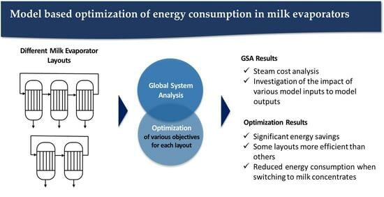
This work examines to what extent the evaporation process can be optimized in terms of energy consumption when TVR and MVR units are incorporated into the evaporator system, as well as which one is more economical. To this end, five different Cases of evaporator layouts are investigated using a global system analysis (GSA) and an advanced optimization approach. Each layout utilizes a TVR or MVR unit. GSA is employed to revise decisions to improve system robustness and reduce parameter uncertainty. The uncertainty analysis allowed the investigation of the impact of design and operational decisions and environmental inputs on Key Performance Indicators (KPIs). Moreover, this study investigates to what extent switching from milk powders to new products known as milk concentrates affects the energy consumption in the evaporation process. Afterward, Cases 1–4 are optimized under five different objective scenarios, some of which examine different end-product specifications (30, 35 or 50% solid content). Steam economy, energy consumption profile, and heat transfer areas are assessed and compared. Finally, it evaluates whether the use of MVR or TVR is more cost-effective for the milk evaporation process based on current steam and electricity prices, economic trends, and costs of steam generated from renewable energy sources. The results of optimization and uncertainty analysis serve as a valuable tool for engineers investigating alternative strategies to improve the energy efficiency of the milk evaporation process. These findings reveal the conditions, operational parameters, and end-product specifications under which each of the investigated milk processing strategies and layouts proves to be cost-effective. Furthermore, the optimization results offer insights into key evaporator design variables, including tube length and diameter, providing practical guidance for process designers aiming to implement TVR or MVR technologies in milk treatment.

The main advances of this work are summarized in

Table 1. Advancements of the present work compared to the literature.

Contributions	Mathematical Modelling	Energy Consumption Optimization Strategy Applied		Heat Source Examined
		MVR	TVR	Renewable based steam
[4]	✓ 1	✕ 2	✕	✓
[5]	✓	✓	✕	✕
[7]	✓	✕	✓	✕
[8]	✓	✓	✓	✕
[10,11]	✓	✕	✕	✕
[12]	✓	✕	✓	✕
[13]	✓	✕	✕	✕
[16]	✓	✕	✕	✕
[18]	✓	✕	✕	✕
[19]	✓	✕	✕	✕
[20]	✓	✕	✓	✕
Proposed approach	✓	✓	✓	✓

¹ ✓ Indicates that a subject area is examined. ² ✕ Indicates that a subject area is not examined.

. To the authors’ knowledge, there is no other literature that compares MVR and TVR in terms of performance and energy consumption in a milk evaporation system. Moreover, the proposed approach examines multiple heat sources of steam (including renewable ones) within multistage evaporator systems with TVR, while no other literature examines this combination.

The remainder of the article is structured as follows: Section 2 describes the material composition along with some of its properties. A detailed presentation of the mathematical model that describes the operation of a falling film evaporator is also described in this section of the paper. Section 3 presents the examined evaporator layouts. The results of the global system analysis and optimization are also presented and thoroughly discussed in Section 3. Finally, Section 4 summarizes the concluded remarks emerging from the study and provides a guideline for potential future work.

2. Materials and Methods

2.1. Milk Composition and Properties

This section provides information about milk properties and conditions. In the present study, the analysis of FFEs is applied to the milk evaporator process, while the thermo-physical properties of the food vary with composition. Two different composition profiles of whole milk before evaporation are examined (

Table 2. Whole milk composition.

Whole Milk Components [21]	Weight (%) [21]	Whole Milk Components [5]	Weight (%) [5]
Water	87.4	Water	87
Carbohydrates	4.9	Fat	4
Proteins	3.5	Protein	3.4
Fat	3.5	Lactose	4.8
Ash	0.7	NaCl	0.4
		KCl	0.4

), while

Table 3. Equations for properties calculation.

Property	Equation *
Specific heat capacity [20]	$c_p={\displaystyle {\displaystyle \sum }_j}{c}_p{}_j{x}_j$	$\left(1\right)$
Thermal conductivity [20]	$k=\rho {\displaystyle {\displaystyle \sum }_j}\frac{{\kappa }_j{x}_j}{{\rho }_j}$	$\left(2\right)$
Density [20]	$\frac{1}{\rho }={\displaystyle {\displaystyle \sum }_j}\frac{x_j}{{\rho }_j}$	$\left(3\right)$

* Where $x_j$ is the component $j$ mass fraction.

summarizes equations for the calculation of properties in the mixture. Thermodynamic and physical properties, such as specific heat capacity $c_p$, thermal conductivity $k$, and density, $\rho$, of ‘pseudo’ milk are modeled using the process simulator, and average values are compared to the literature. The results are summarized in

Table 4. Properties of whole milk before evaporation at 4 °C, 101 kPa.

Property	Value [20]	Value [5]	Simulated Data
Density $\left(\rho \right)$	$1020\mathrm{kg}/{\mathrm{m}}^3$	$1021\mathrm{kg}/{\mathrm{m}}^3$	$1017.9\mathrm{kg}/{\mathrm{m}}^3$
Specific heat capacity $\left(c_p\right)$	$3850\mathrm{J}/\mathrm{kg}℃$	$3830\mathrm{J}/\mathrm{kg}℃$	$3790\mathrm{J}/\mathrm{kg}℃$
Thermal conductivity $\left(k\right)$	$0.53\mathrm{W}/\mathrm{m}℃$	$0.53\mathrm{W}/\mathrm{m}℃$	$0.52\mathrm{W}/\mathrm{m}℃$

.

2.2. Mathematical Model

The concentration of milk in this study is focused on falling film evaporators. In this process, the milk, with a temperature close to its boiling point, is introduced in a uniform manner at the upper section of the inner surface of a tube. These tubes are arranged side by side, fixed in place, and surrounded by a jacket. As the milk descends within each tube, it forms a thin film and undergoes boiling as a result of the heat exchange with the steam. The concentrated liquid is collected at the lower part of the equipment, while the remaining portion is separated from the steam in a subsequent separator. In evaporators equipped with multiple effects, the concentrated liquid is pumped to the next stage, while the steam serves the purpose of heating the subsequent effect [2].

A dynamic model of a simple falling-film evaporator is developed in this section. The model examines the flash calculations of liquid entering the evaporator, its distribution via distributor plates, and its evaporation as it flows downwards through pipes. The model has been developed based on the following assumptions:

• It is assumed that the product immediately reaches its boiling temperature once it passes above the distributor plate, with either steam flashing or condensing.
• All the heating steam condenses at its saturation temperature. The heat released during condensation is utilized to preheat and evaporate the feed stream.
• The pressure difference on the steam side is insignificant, thus resulting in a constant temperature on the steam side.
• The unit is assumed to be perfectly mixed at all times, implying there are no spatial variations in intensive properties within it.
• A steady state balance is applied to the tube flow, but the mass holdup of liquid on the distributed plate is calculated.
• No fouling is considered in the evaporator.

2.2.1. Mass Balance

The rate of change of the mass holdup, $M$, of any given species in phase $p$ in the unit is given by Equation (4):

$$\frac{d{M}_{i,p}}{dt}={\displaystyle \sum }_{j=1}^{N_{inlet}}{F}_{j,p}^{in}·w_{i,j,p}^{in}-F_p^{out}·w_{i,p}^{out}+{\displaystyle \sum }_{p_n\ne p\in P}{R}_{p/p_{n,}i}, \forall i\in I, \forall p\in P$$

(4)

where $F_{j,p}^{in}$is the mass flowrate of the j^th feed stream in phase p, $w_{i,j,p}^{in}$ is the mass fraction of species i in the j^th feed stream in phase p, $F_p^{out}$ is the mass flowrate of material phase p in the outlet stream, $w_{i,p}^{out}$ is the mass fraction of species i in the outlet stream of phase p and $R_{p/p_{n,}i}$ is the rate of mass transfer between the phase p and the phase p_n.

Assuming that the unit is perfectly mixed, the composition of any outlet stream is the same as the composition within the unit:

$$w_{i,p}^{out}=w_{i,p},\forall i\in I,\forall p\in P$$

(5)

where $w_{i,p}$is the mass fraction of species i in phase p in the unit.

The composition of material within the unit is given by Equations (6) and (7):

$$w_{i,p}=\frac{M_{i,p}}{M_{total,p}},\forall i\in I,\forall p\in P$$

(6)

$$M_{total,p}={\displaystyle \sum }_{i\in I}{M}_{i,p},\forall i\in I,\forall p\in P$$

(7)

where $M_{p,total}$is the total holdup of material in phase p within the unit.

2.2.2. Energy Balance

The rate of accumulation of enthalpy, $H$, within the unit, is given by Equations (8) and (9):

$$\frac{dH}{dt}={\displaystyle \sum }_{j=1}^{N_{inlet}}{\displaystyle \sum }_{p\in P}(F_{j,p}^{in}·h_{j,p}^{in})-{\displaystyle \sum }_{p\in P}(F_p^{out}·h_p^{out})-R_{p/p_{n,}i}{h}_{p/p_{n,}i}+Q_{trans}$$

(8)

$$H={\displaystyle \sum }_{p\in P}(M_{total,p} ·h_p)$$

(9)

where $h_p$is the specific enthalpy of the material in the unit in phase p, $h_{j,p}^{in}$ is the specific enthalpy of the j^th feed stream in phase p, $h_p^{out}$ is the specific enthalpy of the outlet stream in phase p, $h_{p/p_{n,}i}$ is the enthalpy of phase change between phase p and phase p_n, and $Q_{trans}$ is the enthalpy transferred into the unit through the boundary due to heat loss, heating, and so forth.

Due to the assumption that the unit is perfectly mixed, the specific enthalpy of each of the outlet streams is equal to the specific enthalpy of the material within the unit:

$$h_p^{out}=h_p$$

(10)

The specific enthalpy is assumed to be a function of the composition and temperature, $T$, of the material within the unit:

$$h_p=h_p\left(T,T_{ref,}{w}_{i,p}\right),\forall p\in P$$

(11)

2.2.3. Heat Transfer Rate

The total heat transfer rate, $Q_{trans}$, is the sum of energy transfer by steam, $Q_{heating}$ and energy loss, $Q_{loss}$, to the environment:

$$Q_{trans}=Q_{heating}+Q_{loss}$$

(12)

$$Q_{heating}=UA\Delta {{\rm T}}_{lm}$$

(13)

$$A=\pi D_{i}NL$$

(14)

$$\Delta T_{lM}=\frac{\Delta {{\rm T}}_1-\Delta {{\rm T}}_2}{\ln \left(\frac{\Delta {{\rm T}}_1}{\Delta {{\rm T}}_2}\right)}$$

(15)

where $U$ is the overall heat transfer coefficient, $A$ is the heat transfer area, $N$ is the number of tubes, $L$ is the length of the tubes, and finally $\Delta {\rm T}$ and $\Delta {{\rm T}}_{lm}$ are the linear and logarithmic temperature differences, respectively.

2.2.4. Flow through Distribute Plate

The distribute plate is an inserted plate that distributes the product stream evenly around the inner periphery of the evaporator tubes. Aside from the liquid holes that allow liquid to pass through, there are also openings to let steam flow through the plate. Two designs for vapor transport through the distribute plate are considered:

• Plate with upstanding vapor tubes.
• Plate with an upstanding rim at the edges of the circular plate and a ring-shaped gap between the plate and evaporator body.

The vapor flowing downwards or upwards through the distributing plate causes a vapor pressure drop, while the liquid flowing downwards through the distributing plate and liquid holdup above the plate causes a liquid pressure drop.

The vapor flows through the plate, ${\dot{F}}_{vap}$, for plate design with upstanding vapor tubes is expressed by the following relation.

$${\dot{F}}_{vap}=N_{vap tube}·\frac{\pi }{4}{d}_{vap tube}^2{\rho }_{vap}{u}_{vap}$$

(16)

$$\Delta P_{vap}=\left(1+f_{f,vap}\frac{L_{vap tube}}{d_{ vap tube}}\right)·\frac{1}{2}{\rho }_{vap}{u}_{vap}^2$$

(17)

where $N_{vap tube}$ is the number of vapor uprising tubes, $d_{vap tube}$ is the diameter of each uprising tube, $L_{vap tube}$ is the length of each tube, ${\rho }_{vap}$ is the vapor density above the plate, $f_{f,vap}$ is the vapor friction factor, and $\Delta P_{vap}$ is the vapor pressure drop.

The vapor flow through the plate for plate design with an upstanding rim at the edges is expressed by Equations (18) and (19):

$${\dot{F}}_{vap}=\frac{\pi }{4}(d_{out}^2-d_{in}^2){\rho }_{vap}{u}_{vap}$$

(18)

$$\Delta P_{vap}=\left(1+f_{f,vap}\frac{h_{rim}}{d_{ out}-d_{ in}}\right)·\frac{1}{2}{\rho }_{vap}{u}_{vap}^2$$

(19)

where $d_{out}, d_{in}$ are the diameter of the evaporator body and the plate, respectively, and $h_{rim}$ is the height of the outer rim.

The liquid flows through the plate, ${\dot{F}}_{liq}$, is expressed by Equations (20) and (21):

$${\dot{F}}_{liq}=N_{liq hole}·\frac{\pi }{4}{d}_{liq hole}^2{\rho }_{liq}{u}_{liq}$$

(20)

$$\Delta P_{liq}=\left(1+f_{f,liq}\frac{h_{plate}}{d_{liq hole}}\right)·\frac{1}{2}{\rho }_{liq}{u}_{liq}^2$$

(21)

where $N_{liq hole}$ is the number of liquid holes, $d_{liq hole}$ is the diameter of liquid holes, $h_{plate}$ is the thickness of the distributed plate, ${\rho }_{liq}$ is the liquid density above the plate, $v_{liq}$ is the liquid flow velocity through the plate, $f_{f,ilq}$ is the liquid friction factor, and $\Delta P_{liq}$ is the liquid pressure drop.

2.2.5. Liquid Flow through Pipes

The wetting rate, $\Gamma$, of a falling film evaporator tube is correlated to the liquid mass flow of the tube, ${\Phi }_m$ and the tube diameter $D_{tube}$ using:

$$\Gamma =\frac{{\Phi }_m}{\pi D_{tube}}$$

(22)

The Reynolds number, $Re$, in the falling film evaporation used in empirical relations, is defined by Equation (23):

$$Re=\frac{\Gamma }{\mu }$$

(23)

where $\mu$is the liquid dynamic viscosity.

The liquid characteristic length, $l_c$, is given as:

$$l_c={\left(\frac{{\mu }^2}{{\rho }^{2}g}\right)}^{\frac{1}{3}}$$

(24)

where $\rho$is the liquid density and $g$ is the gravity acceleration.

The film thickness, $\delta$, is calculated by Equation (25):

$$\delta =\left\{\begin{array}{c}{\left(\frac{2.4{\mu }^2}{{\rho }^{2}g}\right)}^{\frac{1}{3}}R{e}^{\frac{1}{3}}=1.34l_{c}R{e}^{\frac{1}{3}} Re<400\\ 0.302{\left(\frac{3{\mu }^2}{{\rho }^{2}g}\right)}^{\frac{1}{3}}R{e}^{\frac{8}{15}}=0.436l_{c}R{e}^{\frac{8}{15}} Re \ge 400\end{array}\right\}$$

(25)

Assuming that the film thickness is small compared to the tube diameter, the liquid velocity downwards on the tube, $u$, and the residence time, $t$, for liquid flow to the bottom are calculated based on Equations (26) and (27):

$$u=\frac{\Gamma }{\rho \delta }$$

(26)

$$t=\frac{L_{tube}}{u}$$

(27)

2.2.6. Boiling Point Elevation

The boiling point elevation of a solution can be calculated by combining the laws of Raoult and Clausius Clapeyron:

$$\Delta {\rm T}=-\frac{R{T}_{water}^2}{H_{evap}{M}_{w,water}}\ln (X_{water})$$

(28)

where $R$ is the gas constant, $T_{water}$ is the boiling temperature of water, $H_{evap}$ is the heat of evaporation, $M_w$ is molar weight and $X_{water}$ is the molar fraction of water in the solution.

It is assumed that fat does not dissolve in the solvent and, therefore, does not affect the boiling point. The molar fraction of water in the fat-free product can therefore be calculated:

$$X_{water}=\frac{\frac{f_{m,water}}{M_{w,water}}}{{{\displaystyle \sum }}_{i\in com{p}_{fatfree}}\frac{f_{m,i}}{M_{w,i}}}$$

(29)

where $f_m$ denotes for the mass fraction and $com{p}_{fat free}$ refers to all but fat components.

2.2.7. Liquid Friction Factor

The most widely used correlation for liquid friction factor is the Wallis correlation for annular falling film, and it is incorporated into the model for better prediction of the liquid friction factor [19].

$$f_{f liq}=0.05·\left(1+300·\frac{\delta }{D_i}\right)$$

(30)

2.2.8. Energy Cost

In order to compare the energy consumption of TVR and MVR, the variable energy cost is used, which is defined by Equations (31) and (32). When employing TVR technology, the annual cost is given as:

$$Energy cost=Stea{m}_{unit}cost·Stea{m}_{flowrate}·hour{s}_{peryear}$$

(31)

For MVR, the annual energy cost is expressed as:

$$Energy cost=Electricit{y}_{unit}cost·Powe{r}_{consumption}·hour{s}_{peryear}$$

(32)

The current price of steam based on natural gas is 20 USD/t [22]. According to Eurostat [23], the electricity unit cost for non-household users in 2023 is 0.21 USD/kWh. The operating hours per year are considered as 7920 h/yr; thus, variable Energy cost refers to annual energy cost.

2.3. Solution Techniques

In the present study, global system analysis and optimization are conducted in gPROMS^TM FormulatedProducts [24] version 2.3.0 from Siemens Process Systems Enterprise. A database containing physical and thermodynamic properties of milk components is developed using gPROMS FormulatedProducts Utilities. The Algebraic-Differential equations are integrated with respect to time using the DASOLV solver, and the dynamic optimization is conducted by employing the Control Vector Parameterization method. No computational issues emerged during the simulation and optimization runs.

3. Results and Discussion

In this section, the GSA and optimization results are presented and thoroughly discussed. It is worth mentioning at this point that the study is limited to a simulation scale. The lack of industrial and experimental data prevents a direct comparison between experimental and simulation results. Despite the acknowledged limitations, the attained results are still exceptionally advantageous for the theoretical exploration of the energy consumption minimization problem during the milk evaporation process and can potentially provide insights into the efficiency and cost-effectiveness of evaporator systems that incorporate either TVR or MVR and vary in the number of effects they comprise.

3.1. Case Studies

Five different evaporators are considered, combined with different energy consumption minimization strategies, namely MVR and TVR. These process alternatives are often met in the food processing industry. The design characteristics of the evaporators of each layout are provided in Tables S1–S4 of the Supplementary Materials. Cases 1 and 5 represent industrial-scale evaporator systems, while Cases 2–4 are related to pilot-scale systems (1000 kg/h).

3.1.1. Case 1

Case 1 examines the operation of a local South African plant that consists of two evaporation chambers (referred to as effects), a TVR system for vapor recycling from 1st stage to the same stage, and a condenser to remove heat and keep the unit under vacuum [19]. The system is displayed in Figure 1.

3.1.2. Case 2

Raw milk enters the preheater tubes of the 2nd and the 1st evaporator before entering the 1st evaporator chamber, as shown in Figure 2. As the evaporation process continues in FFE1, the generated steam works as the heating medium in the 2nd evaporator effect, where the semi-concentrated product is further evaporated, resulting in the end-product (concentrate). The steam generated in the 2nd effect is recycled to the TVR, where fresh steam is also added, increasing its pressure before entering the 1st effect.

3.1.3. Case 3

In Case 3 (Figure 3), 1000 kg/h raw milk is fed to the preheater tubes of the 3rd, 2nd, and 1st evaporator effect subsequently before entering the 1st evaporator chamber. As the evaporation process continues in FFE1 and FFE2, the generated steam at each effect works as the heating medium for the next one, with the whole process resulting in the end product (concentrate). The steam generated in the 3rd effect is recycled to TVR, where fresh steam is added, increasing its pressure before entering the 1st effect.

3.1.4. Case 4

In Case 4 (Figure 4), 1000 kg/h raw milk is fed in a single-stage evaporator, with no addition of external steam. The evaporation occurs only by recompressing the vapor generated and recycling it to the unit by an MVR. The only source of energy needed in this process is electricity.

3.1.5. Case 5

Case 5, presented in Figure 5, examines the proposed evaporation system by Galvản-Ángeles et al. [20]. The system has four effects with co-current flow, and it is capable of processing 16,000 kg/h of whole milk. The arrangement employs a TVR unit, recycling vapor from the 2nd to the 1st stage of evaporation.

3.2. Global System Analysis

GSA allows for a systematic exploration of the relative impact of input parameters on model output responses. The fundamental principle of GSA involves sampling from a defined particulate system. This entails extracting various values for individual parameters and calculating the corresponding output values. Uncertainty analysis is employed using the Monte Carlo method to determine the effects of uncertain input parameters on the system responses. The Monte Carlo method involves performing multiple model evaluations using either deterministic or probabilistic distributions. The resulting output values from these evaluations are then utilized to assess the impact of the system’s uncertainty. In this study, uncertainty analysis is conducted to assess key decision space optimal areas rather than single optimal values of the degrees of freedom. Uncertainty analysis is performed for all Cases, implementing the standard Monte Carlo method. Quasi-random (Sobol) sampling is used as the sample generation method, which fills the space uniformly, as it has proved to be efficient for medium-sized problems and a high number of samples. The number of uncertainty scenarios is set to 1000.

3.2.1. Steam Cost Analysis

This study also considers the uncertainty of steam price. Steam can be generated from a wide range of sources, including fossil fuels such as natural gas (main source), as well as renewable energy sources like lignocellulosic biomass, solar, and waste. The rise of renewable energy sources presents an opportunity to examine the prices of steam generated from these sources, taking into account their future values, which could potentially fluctuate by around ±40%. Pérez-Uresti et al. [22] evaluated the production cost of renewable-based steam, including solar, lignocellulosic biomass, and biogas. Results showed that considering the current price of steam based on NG, lignocellulosic biomass offers better perspectives to become a competitive resource when compared to the other two sources. More specifically, the evaluated production cost of steam is as follows: NG-based steam costs 16.8 USD/t, biomass-based steam costs 20.4 USD/t, solar-based steam costs 32.5 USD/t, and biogas-based steam costs 27.4 USD/t.

The analysis conducted in this work takes into account future values of those described above, which could potentially fluctuate by a maximum of 40%, to determine to what extent and in what circumstances renewable-based steam can become a competitive resource compared to natural gas. The specific analysis involves only Case 1 because the same pattern of results would emerge when investigating the rest of the Cases.

Table 5. Potential steam price fluctuations for different steam generation sources.

	−40%	−30%	−20%	−10%	0%	+10%	+20%	+30%
	Cost (USD/t)
Biomass-based steam	12.2	14.3	16.3	18.3	20.4	22.4	24.4	26.5
Solar-based steam	19.5	22.8	26	29.3	32.5	35.8	39	42.3
Biogas-based steam	16.5	19.2	21.9	24.7	27.4	30.2	32.9	35.6
NG-based steam	10.1	11.8	13.5	15.1	16.8	18.5	20.2	21.9

summarizes the prices examined to determine to what extent and in what circumstances renewable-based steam can become a competitive resource compared to natural gas.

Uncertainty analysis results related to the operating annual cost of evaporation depending on various steam sources and future steam unit costs are summarized in

Table 6. Minimum and maximum annual cost values of the evaporation process depending on the steam source.

	−40%	−30%	−20%	−10%	0%	+10%	+20%	+30%
Minimum Annual Cost (USD × 103)
Biomass-based steam	82.5	96.2	110	124	137	151	165	179
Solar-based steam	132	154	175	197	219	241	263	285
Biogas-based steam	111	130	148	167	185	204	222	241
NG-based steam	68.1	79.4	90.8	102	113	125	136	147
Maximum Annual Cost (USD × 103)
Biomass-based steam	279	325	372	418	465	511	558	604
Solar-based steam	445	519	593	668	742	816	890	964
Biogas-based steam	375	438	500	563	626	688	751	814
NG-based steam	230	269	307	345	384	422	460	499

. Despite natural gas being currently the most economical choice, a future possible reduction of biomass-based steam cost by only 20% (or more) would lead to lower values of annual expenditure for the evaporation process of Case 1, compared to the nominal scenario of using NG-based steam. Biogas-based steam and solar-based steam do not seem economically attractive after the analysis, as a reduction of 40% for the former or over 50% for the latter would be needed in order for those sources to be competitive with natural gas. However, as predictions indicate a rise in natural gas prices, renewable-based steam can become more and more competitive both for environmental and economic reasons.

3.2.2. Global System Analysis—Case 1

The factors used for the uncertainty analysis for Case 1 are the steam cost, the TVR discharge pressure, the TVR suction ratio (defined as the suction steam mass flowrate to the fresh steam mass flowrate, and the feed temperature. The lower and upper bounds, along with the probability distribution of the factors, are presented in Table S5 of the Supplementary Materials.

Figure 6a illustrates the variation of the concentrate mass fraction of water versus feed temperature and TVR discharge pressure. It is clear that higher outlet pressures and higher feed temperatures result in a lower mass fraction of water in the end product, thus leading to a product with a higher dry mass fraction. Higher feed temperatures can be achieved by preheating the feed stream.

As shown in Figure 6b, the TVR suction ratio illustrates the largest effect on the steam economy. The steam economy is defined as the sum of the mass flowrate of the evaporated water of each evaporator effect divided by the feed mass flowrate (fresh steam). Suction ratios over 1.3 result in higher values of yield, while high feed temperatures along with suction ratios over 1.6 can result in a steam economy close to 4. On the contrary, fresh steam mass flowrate is mostly affected by TVR discharge pressure, as shown in Figure 6c. Low values of discharge pressure result in minimum mass flowrates (around 600 kg/h steam), whereas high outlet pressures along with low suction ratios can result in even 3200 kg/h steam, which quintuple the cost of evaporation.

Figure 6d,e illustrates that TVR discharge pressure affects both the pressure of the concentrate product and the solid mass fraction of the FFE1 outlet product. Higher discharge pressure values can be mutually beneficial for achieving greater vacuum (lower concentrate pressure) and resulting in more concentrated products (lower moisture content), which is ideal for downstream spray drying processes.

3.2.3. Global System Analysis—Case 2

Uncertainty analysis is performed for Case 2 to examine the effect of key factors on various key responses (model variables). The factors of this analysis are the TVR discharge pressure, the TVR suction ratio, and the feed temperature. Information about the factors of this case is provided in Table S6 of the Supplementary Materials.

As responses of several variables are discussed in the GSA of Case 1, which also includes two evaporator effects with TVR in plant scale, in this section, it is worth highlighting differences in responses related to laboratory scale or responses of other important variables. Figure 7a indicates that on a laboratory scale, higher values of steam economy can be achieved as the lower and upper bounds of this variable are higher than that of Figure 6b (1.4 as opposed to 1 and 5.2 as opposed to 5, respectively).

Figure 7b illustrates that although the lower bounds of solid mass fraction after the first evaporation effect are the same as Figure 6e (plant scale), the upper bounds are remarkably higher (almost 0.45), indicating that a single evaporation effect is sufficient in some cases depending on the underlying product specifications.

Figure 7c illustrates the annual cost of steam versus feed temperature and TVR outlet pressure. The steam unit cost is fixed at 20 USD/t (NG—based steam) while the operating hours are 7920 h. The results show that the operating conditions can greatly affect the annual cost, ranging from 6000 to 44,000 USD/yr. However, these values are related to different end-product specifications, so the final optimization results are presented in Section 3.3.2.

3.2.4. Global System Analysis—Case 3

Uncertainty analysis is performed for Case 3, with the factors used in this analysis being the same as those used for Case 2. The derived results are illustrated in Figure 4. Figure 8a shows the variation of steam economy versus feed temperature and suction ratio in more detail. It is demonstrated that an arrangement of 3 evaporator effects with TVR leads to high steam economy values compared to Case 2. Specifically, the lower and upper bounds of steam economy in Case 3 are 2.4 and 7.6, respectively, as opposed to 1.2 and 5.2 in Case 2. Figure 8b and Figure 8c illustrate the variation of the dry mass fraction at the FFE1 and FFE2 evaporator tube outlets, respectively, while Figure 8d shows the water mass fraction of the concentrate (end product). Higher values of TVR discharge pressure result in more concentrated products, while FFE1 liquid product can have 13% to 18% solid content in Case 3 as opposed to 14% to 46% of that of Case 2. In Case 3, the maximum solid concentration of FFE2 outlet product is 26% which implies that the evaporation process is mainly enhanced in the 3rd effect, rather than the 1st one in the case of two evaporator effects with TVR (Case 2).

Figure 8e illustrates the annual cost of steam versus TVR suction ratio and TVR outlet pressure. The steam unit cost is fixed at 20 USD/t (NG—based steam), and the operating hours are 7920. The results show that higher values of outlet pressure combined with low values of suction ratios can greatly increase the annual cost. On the other hand, Case 3 results in a lower steam annual cost than that of Case 2. Specifically, the analysis of Case 2 resulted in operating costs of 6000–44,000 USD/yr (Figure 7c) as opposed to 5000–32,000 USD/yr of Case 3.

3.2.5. Global System Analysis—Case 4

The factors considered for the uncertainty analysis for Case 4 are the MVR compression ratio and the feed temperature. The compression ratio is expressed as the outlet steam pressure divided by the inlet steam pressure. The lower and upper bounds, along with the probability distribution of the factors, are provided in Table S7 of the Supplementary Materials. The results are shown using various figures, while TVR and MVR operations can be assessed and compared.

Figure 9a illustrates the moisture mass fraction of concentrate versus feed temperature and MVR compression ratio. Higher values of compression ratio and feed temperature result in more concentrated products, and compression ratios over 1.25 lead to efficient evaporation (a solid mass fraction over 0.3). Consequently, the operating cost of evaporation rises with higher values of compression ratios (Figure 9b).

It is worth mentioning that the average electricity unit cost is fixed at 0.21 USD/kWh, and the operating hours are 7920. The results show that the operating conditions can greatly affect the annual cost ranging from 2000 to 34,000 USD/yr. Compared with Cases 2 and 3, Case 4 leads to the lower minimum cost (2000 USD/yr as opposed to 5000 USD/yr and 6000 USD/yr of Cases 3 and 2, respectively) and an intermediate upper bound (34,000 USD/yr as opposed to 32,000 USD/yr and 44,000 USD/yr of Cases 3 and 2, respectively). However, these values are related to different end-product specifications, and a comprehensive comparison is made using dynamic optimization techniques. The results are presented in Section 3.3.4.

Finally, Figure 9c depicts the variation of concentrate product pressure versus MVR compression ratio and feed temperature. The latter one illustrates the greatest impact on the achieved vacuum, as lower values of feed temperature result in a greater vacuum (around 2500 Pa pressure). However, as shown in Figure 9c, an end-product dry mass fraction over 0.5 cannot be achieved for feed temperatures lower than 40 °C.

3.2.6. Global System Analysis—Case 5

Uncertainty analysis is finally performed for Case 5 to examine the effect of the split fraction, TVR suction ratio, and feed temperature (factors) on various KPIs. More information about the studied factors is provided in Table S8 of the Supplementary Materials. As Case 5 involves a plant scale process with four evaporator effects by recycling steam from the 2nd effect to TVR, different recycling fractions (split fractions) can be examined. Furthermore, both plant and laboratory processes can be evaluated.

Figure 10a illustrates the water mass fraction of the concentrate product versus the feed temperature and split fraction. Empty spaces indicate that simulations cannot be provided in certain areas; thus, recycling over 60% of FFE2′s steam (providing FFE3 with the remainder of steam) while keeping the feed temperature below 50 °C results in failed simulations. However, higher feed temperatures and lower split fractions enhance the evaporation process as the concentrated product has lower moisture content. This implies that by providing more steam to the next evaporator effect, the evaporation is more enhanced than recycling larger quantities of steam in the TVR unit.

Figure 10b shows the variation of yield versus the feed temperature and split fraction. The evaporation yield is defined as the mass flowrate of the end product (concentrate) divided by the feed mass flowrate (fresh steam). It follows the exact opposite pattern with Figure 10a, as higher feed temperature and lower split fraction result in lower product yield. However, despite producing smaller amounts of concentrated product, the lower yield indicates products with reduced moisture content.

Figure 10c illustrates the annual steam cost (steady-state values) versus the TVR suction ratio and split fraction. Suction ratio influences steam cost the most, as higher values of suction ratio result in higher costs, ranging from 370,000–500,000 USD/yr. It is demonstrated that there is a relatively linear relationship between laboratory and plant-scale evaporation processes.

Table 7. Minimum and maximum values of dry mass fraction of each effect outlet attained by the uncertainty analysis.

Variable	Minimum (×10−1)	Maximum (×10−1)
FFE1 Outlet dry mass fraction (kg/kg)	1.62	1.69
FFE2 Outlet dry mass fraction (kg/kg)	2.25	2.54
FFE3 Outlet dry mass fraction (kg/kg)	2.78	3.59
FFE4 Outlet dry mass fraction (kg/kg)	3.41	6.10

summarizes the minimum and maximum values of the outlet dry mass fraction of each effect resulting from the uncertainty analysis. It is concluded that for each of the first three evaporator effects, there is a narrow range of dry mass fraction. The FFE1 liquid product outlet dry mass fraction is limited to 0.17 while the FFE2 liquid product outlet dry mass fraction ranges from 2.25 $\times$ 10⁻¹ to 2.54 $\times$ 10⁻¹. It is thus indicated that the evaporation process is mainly enhanced in the 3rd and 4th evaporator effects with maximum outlet product dry mass fractions of 0.36 and 0.61, respectively.

3.3. Dynamic Optimization

Depping et al. [25] investigated whether switching from milk powders to new products known as milk concentrates diminishes the overall environmental impact along the supply chains of dairy-containing products. For relevant environmental indicators such as cumulative energy demand, global warming potential, eutrophication potential, and acidification potential, concentrates are found to have a lower environmental impact than powders, even if the former are trucked up to 1000 km. To this end, as drying milk into milk powders is a highly energy-intensive process and energy demand per kilogram of water removed rises nonlinearly with increasing dry-matter content [26], it is crucial to investigate the amount of energy saved when switching to milk concentrates. This can be performed by optimizing the annual operating cost of steam or electricity used in the evaporation process with respect to different product specifications. The new products considered are shelf-stable milk concentrates, which are compared to the current benchmark product, milk powders. Specifically, three concentrated dry mass contents are considered: 30%, 35%, and 50%. The first two are related to concentrates, and the third one is necessary for milk powder production before drying.

The optimization of the process aims to maximize or minimize an objective function subject to design and operating constraints related to the nature of the process, the end-product specifications, or the environment. In this work, advanced dynamic optimization techniques are employed for Cases 1–4, aiming to increase process performance while minimizing operating costs (in case of existing industries) or total costs (in case of new plant design) under different end-product specifications. Specifically, Cases 1–4 are optimized under six scenarios, described in

Table 8. Optimization scenarios examined—Cases 1–4.

Scenario	Objective Function	Product Quality Specifications
1	Minimization of annual steam cost (USD/yr)	Product dry mass fraction = 0.5
2	Minimization of annual steam cost (USD/yr)	Product dry mass fraction = 0.35
3	Minimization of annual steam cost (USD/yr)	Product dry mass fraction = 0.30
4	Maximization of yield	Product dry mass fraction = 0.5
5	Minimization of total cost	Product dry mass fraction = 0.5
6	Maximization of yield	0.3 < Product dry mass fraction < 0.5

, along with product quality specifications. Optimization results are compared with the nominal Cases expressed by simulation results to highlight the benefits of optimization.

In many cases, the optimization is applied to already existing industries, the design of which is fixed. However, it is worth examining an objective function that includes annualized fixed cost along with the operating cost of steam for the cases of new plant design, capacity expansion, or even the examination of capital investment due to trade-offs between capital and operating costs. Equation (33) represents the total annualized cost [27].

$$Total cost=CCF·F_{BM}·\left({\displaystyle \sum }_{i=1}^n{10}^{3.91+0.86\mathit{log}\left(A_i\right)-0.0088\left[log(A_i\right){]}^2}\right)+stea{m}_{unit}cost·Stea{m}_{flowrate}·hour{s}_{peryear}$$

(33)

where $CCF\left(=1/3\right)$ is the fixed capital charge coefficient, $FBM \left(=2.45\right)$ is the installed equipment coefficient, and n is the number of evaporator effects. Operating hours are fixed at 7920 h.

The optimization variables represent the degrees of freedom of the optimization problem. For Cases 1–3 and optimization scenarios 1–4,6, the optimization variables are (a) the TVR—Pressure (discharge), (b) the TVR—Suction ratio, and (c) Feed Temperature, while for optimization scenario 5, the optimization variables are: (a) FFE1 tube inner diameter, (b) FFE1 tube length, (c) FFE2 tube inner diameter and (d) FFE2 tube length. The optimization variables for Case 4 and scenarios 1–4,6 are (a) MVR-Adiabatic efficiency, (b) MVR-Compression ratio, and (c) Feed temperature. Finally, for Case 4 and Scenario 5, the optimization variables are (a) FFE1 tube inner diameter and (b) FFE1 tube length. More comprehensive information regarding the optimization variables, including their upper and lower limits, for every examined case and scenario is provided in Tables S9–S11 of the Supplementary Materials.

The time horizon of interest is fixed at 1 h in all Cases and scenarios, while the optimization variables are time-invariant, and the constraints (equality or inequality) must be satisfied at the end of the time horizon. In each optimization case, a full description of the constraints and optimization results are provided for each scenario.

3.3.1. Dynamic Optimization—Case 1

The constraints imposed on the process optimization and state variables are summarized in

Table 9. Operating constraints for Case 1 optimization.

Constraints	Explanation
$W_W\left(t_f\right)=0.5 \left(\mathrm{or} 0.65\mathrm{or} 0.7\right)$	The final water content must be equal to 0.5 in Scenarios 1,4 and 5, 0.65 in Scenario 2, and 0.7 in Scenario 3.
$10 ℃\le T_{FFE1}\left(t_f\right)\le 70 ℃$	FFE1 temperature should be under 70 °C to mitigate the negative effects of heat on heat-sensitive milk components and prevent the degradation of essential nutrients.
$10 ℃\le T_{FFE2}\left(t_f\right)\le 68 ℃$	The temperature of each evaporator effect must be at least 2 °C lower than the previous one to ensure proper vacuum.
$0.5\le W_W\left(t_f\right)\le 0.7$	Only for Scenario 6, the final water content varies between 0.5 and 0.7

, along with their explanation. The results of the various optimization scenarios for Case 1 are summarized in

Table 10. Optimal values of performance indices, time-invariant optimization variables, and final process variables for each Scenario—Case 1.

Scenario	1	2	3	4	5	6	Non-Optimized
Steam annual cost (USD/yr)	232,000	200,000	182,000	319,000	228,000	261,000	369,000
Total annualized cost (USD/yr)	3.90 × 106	3.86 × 106	3.85 × 106	3.98 × 106	2.33 × 106	3.92 × 106	4.03 × 106
Yield	2.4 × 10−1	3.6 × 10−1	4.2 × 10−1	2.52 × 10−1	2.52 × 10−1	4.2 × 10−1	2.7 × 10−1
TVR—Discharge Pressure (bar)	3.47 × 10−1	3.41 × 10−1	3.38 × 10−1	3.5 × 10−1	3.5 × 10−1	3.42 × 10−1	3.5 × 10−1
TVR—Suction ratio	2	2	2	1.4	2	1.4	1.1
Feed Temperature (°C)	60	60	60	31.8	60	26.7	20
FFE1/FFE2 tube inner diameter (m)	5.08 × 10−2	5.08 × 10−2	5.08 × 10−2	5.08 × 10−2	4.35 × 10−2/ 2.54 × 10−2	5.08 × 10−2	5.08 × 10−2
FFE1/FFE2 tube length (m)	16	16	16	16	17/5	16	16
FFE2 Temperature (°C)	66.7	67.1	66.9	66.7	53.4	67.1	66.9
Concentrate water content	0.5	0.65	0.7	0.5	0.5	0.7	0.54

. In Case 1, the minimum steam annual cost when producing a product with 50% moisture content (necessary for the subsequent spray drying) is 232,000 USD/yr. When the end-product specification is reduced to 35% dry mass content, the annual steam cost decreases by 14% to 200,000 USD/yr (Scenario 2). Further reduction in concentrate dry mass fraction constraint to 30% leads to an approximately 22% reduction in annual steam cost (182,000 USD/yr, Scenario 3). In all examined optimization scenarios, the optimization strategies were able to reduce the annual steam cost to over 37%. Product yield is also affected by the product specifications, as it increases with the rise of product water content. Consequently, higher production rates can be achieved when producing concentrates, as opposed to milk powders, with the same feed flowrate. Feed temperature seems to be optimal at its upper bound in the first three scenarios, indicating that preheated feed streams should be considered.

Energy consumption for a typical evaporator unit comprised of $n$ effects can be approximated as $\frac{2700}{n}$ kJ/kg of evaporated water [28]. Thus, for a 2-stage falling film evaporator system, the energy needed is 1350 kJ/kg. However, in the non-optimized scenario (Case 1), the actual energy consumption per unit of evaporated water is calculated at 814 kJ/kg (0.3 kg steam per kg of evaporated water). This deviation from the literature’s approximate value can be attributed to the utilization of the thermo-compressor (TVR).

Comparing scenarios 4 and 6, high values of product yield cannot be achieved when restricting the product dry mass fraction to 50%, even when maximizing yield. However, when this constraint is relaxed (Scenario 6), the yield can take values up to 0.42 as opposed to 0.25 in Scenario 4.

Regarding the annualized total cost, it is worth considering the optimization of Scenario 5 as opposed to the non-optimized scenario of Case 1. For a new plant design, optimization strategies can result in around a 45% reduction in the total cost. The plant under consideration has 16 m tubes with 5.08 × 10⁻² m inner diameter in both evaporator effects. To minimize the total annualized cost, regarding an expansion of this plant or a new plant design, the optimal values of these dimensions would be 17 and 5 m tube length and 4.35 × 10⁻² and 2.54 × 10⁻² m inner diameter for the 1st and the 2nd evaporator effect, respectively. The total cost is reduced to 232,000 USD/yr for a plant processing 10,600 kg/h raw milk. From the aforementioned results, it is clear that optimal strategies would enhance evaporation in the 1st effect (longer tubes and tube diameter) rather than sticking to the identical design of the two evaporator chambers with moderate dimensions.

3.3.2. Dynamic Optimization—Case 2

The constraints imposed on the process optimization and state variables are the same as those of Case 1 (Table 9). The optimization results are presented in

Table 11. Optimal values of performance indices, time-invariant optimization variables, and final process variables for each Scenario—Case 2.

Scenario	1	2	3	4	5	6	Non-Optimized
Steam annual cost (USD/yr)	21,200	18,900	17,200	30,700	20,700	25,300	30,700
Total annualized cost (USD/yr)	504,000	502,000	501,000	514,000	275,000	509,000	514,000
Yield	2.79 × 10−1	3.6 × 10−1	4.2 × 10−1	2.8 × 10−1	2.52 × 10−1	4.2 × 10−1	2.8 × 10−1
TVR—Discharge Pressure (bar)	3.49 × 10−1	3.45 × 10−1	3.41 × 10−1	3.5 × 10−1	3.5 × 10−1	3.42 × 10−1	3.5 × 10−1
TVR—Suction ratio	2	2	2	1.1	2	1.1	1.1
Feed Temperature (°C)	60	60	60	55.9	60	53.5	55
FFE1/FFE2 tube inner diameter (m)	5.08 × 10−2	5.08 × 10−2	5.08 × 10−2	5.08 × 10−2	5.08 × 10−2 /2.54 × 10−2	5.08 × 10−2	5.08 × 10−2
FFE1/FFE2 tube length (m)	6	6	6	6	5.7/0.6	6	6
FFE2 Temperature (°C)	66.9	67.2	67.4	66.9	20	67.4	66.9
Concentrate water content	0.5	0.65	0.7	0.5	0.5	0.7	0.55

. As Case 2 involves a laboratory/pilot scale evaporation process with TVR, various results can be concluded from Table 11 compared to Case 1 (plant scale). Regarding Case 2, the minimum annual steam cost when producing a product with 35% dry mass content (Scenario 2) is 18,900 USD/yr, indicating a 10.8% reduction from the minimum cost when producing milk powder-restricted products (Scenario 1). A further reduction to the restriction in the concentrate dry mass fraction to 30% led to approximately 18.9% savings in annual steam cost (17,200 USD/yr, Scenario 3). In all scenarios, optimization strategies were able to reduce the annual steam cost to over 31%. Results regarding product yield (Scenario 4 and 6) follow the same trend as Case 1.

The total annualized cost is optimized in Scenario 5 as opposed to the non-optimized scenario of Case 2. The results indicate a 46% reduction in the total cost. The pilot plant under consideration has 6 m tubes with 5.08 × 10⁻² m inner diameter in both evaporator effects. To minimize the total annualized cost, a new laboratory-scale process would select the optimal values of these dimensions to be 5.7 and 0.6 m tube length and 5.08 × 10⁻² and 2.54 × 10⁻² m inner diameter for the 1st and the 2nd evaporator effect, respectively. Thus, the total annualized cost is reduced to 275,000 USD/yr for processing 1000 kg/h raw milk.

In the non-optimized scenario of Case 2, the energy consumption per unit of evaporated water is 734 kJ/kg (equivalent to 0.27 kg of steam per kg of evaporated water), showcasing an improvement over the recorded value for Case 1, which stood at 814 kJ/kg. Notably, the specific energy consumption for a two-stage FFE without a thermo-compressor (TVR) is estimated to be around 1350 kJ/kg, as indicated by the literature [28].

3.3.3. Dynamic Optimization—Case 3

The constraints imposed on the process optimization and state variables are summarized in

Table 12. Operating constraints for Case 3 optimization.

Constraints	Explanation
$W_W\left(t_f\right)=0.5 \left(\mathrm{or} 0.65\mathrm{or} 0.7\right)$	The final water content must be equal to 0.5 in Scenarios 1,4 and 5, 0.65 in Scenario 2, and 0.7 in Scenario 3.
$10 ℃\le T_{FFE1}\left(t_f\right)\le 70 ℃$	FFE1 temperature should be under 70 °C to mitigate the negative effects of heat on heat-sensitive milk components and prevent the degradation of essential nutrients.
$$\begin{gathered} 10 ℃\le T_{FFE2}\left(t_f\right)\le 68 ℃ \\ 10 ℃\le T_{FFE3}\left(t_f\right)\le 66 ℃ \end{gathered}$$	The temperature of each evaporator effect must be at least 2 °C lower than the previous one to ensure proper vacuum.
$0.5\le W_W\left(t_f\right)\le 0.7$	Only for Scenario 6, the final water content can vary between 0.5 and 0.7

, along with their explanation. The results of the various optimization scenarios are summarized in

Table 13. Optimal values of performance indices, time-invariant optimization variables, and final process variables for each Scenario—Case 3.

Scenario	1	2	3	4	5	6	Non-Optimized
Steam annual cost (USD/yr)	15,100	13,000	11,300	22,100	18,900	19,200	22,100
Total annualized cost (USD/yr)	681,000	679,000	677,000	688,000	449,000	685,000	688,000
Yield	2.5 × 10−1	3.5 × 10−1	3.6 × 10−1	2.52 × 10−1	2.5 × 10−1	3.6 × 10−1	2.5 × 10−1
TVR—Discharge Pressure (bar)	3.5 × 10−1	3.42 × 10−1	3.4 × 10−1	3.5 × 10−1	3.49 × 10−1	3.44 × 10−1	3.5 × 10−1
TVR—Suction ratio	2	2	2	1.1	1.37	1.1	1.1
Feed Temperature (°C)	60	60	60	54.9	60	53.6	55
FFE1/FFE2/FFE3 tube inner diameter (m)	5.08 × 10−2	5.08 × 10−2	5.08 × 10−2	5.08 × 10−2	5.08 × 10−2/3.81 × 10−2/ 3.81 × 10−2	5.08 × 10−2	5.08 × 10−2
FFE1/FFE2/FFE3 tube length (m)	6	6	6	6	4.25/ 4.12/ 4.13	6	6
FFE2 Temperature (°C)	67.6	67.9	67.9	67.6	65.4	67.9	67.6
FFE3 Temperature (°C)	65.2	65.8	65.9	65.3	60.9	65.9	65.3
Concentrate water content	0.5	0.65	0.7	0.5	0.5	0.7	0.5

. The results demonstrate that the minimum annual steam cost when producing a product with 50% dry mass content (Scenario 1) is 15,100 USD/yr, while a 13.9% (or more) reduction can be achieved when producing milk concentrates (Scenarios 2 and 3). Optimization strategies were able to reduce the annual steam cost to over 32% compared to the non-optimized scenario of Case 3.

The total annualized cost is optimized in Scenario 5 as opposed to the non-optimized scenario of Case 3. The results indicate an approximately 35% reduction in the total cost. The pilot plant under consideration has 6 m tubes with 5.08 × 10⁻² m inner diameter in all three evaporator effects. To minimize the total annualized cost, a new laboratory-scale process would select the optimal values of these dimensions to be 4.25, 4.12, and 4.13 m tube length and 5.08 × 10⁻², 3.81 × 10⁻², and 3.81 × 10⁻² m inner diameter for effects 1, 2 and 3, respectively. The total annualized cost is therefore reduced to 449,000 USD/yr for processing 1000 kg/h raw milk.

For a typical three-stage FFE (without MVR or TVR), literature [28] indicates that the energy consumed per unit of evaporated water mass is approximately 900 kJ/kg. In Case 3, the specific energy consumption is notably lower at 506 kJ/kg (equivalent to 0.19 kg of steam per kg of evaporated water). The deviation can be attributed once again to the incorporation of TVR technology. Optimization of the Case 3 layout may lead to even lower values of specific energy consumption regarding the optimization scenario examined.

3.3.4. Dynamic Optimization—Case 4

The constraints imposed on the process optimization and state variables are summarized in

Table 14. Operating constraints for Case 4 optimization.

Constraints	Explanation
$W_W\left(t_f\right)=0.5 \left(\mathrm{or} 0.65\mathrm{or} 0.7\right)$	The final water content must be equal to 0.5 in Scenarios 1,4 and 5, 0.65 in Scenario 2, and 0.7 in Scenario 3.
$10 ℃\le T_{FFE1}\left(t_f\right)\le 70 ℃$	FFE1 temperature should be under 70 °C to mitigate the negative effects of heat on heat-sensitive milk components and prevent the degradation of essential nutrients.
$0.5\le W_W\left(t_f\right)\le 0.7$	Only for Scenario 6, the final water content can vary between 0.5 and 0.7

, and the results attained for each optimization scenario are presented in

Table 15. Optimal values of performance indices, time-invariant optimization variables, and final process variables for each Scenario—Case 4.

Scenario	1	2	3	4	5	6	Non-Optimized
Electricity annual cost (USD/yr)	34,300	23,800	19,300	36,000	39,500	20,500	34,600
Total annualized cost (USD/yr)	276,000	265,000	261,000	278,000	251,000	262,000	276,000
Yield	2.52 × 10−1	3.6 × 10−1	4.2 × 10−1	2.52 × 10−1	2.52 × 10−1	4.2 × 10−1	2.6 × 10−1
MVR—Adiabatic efficiency	1	1	1	0.98	1	1	1
MVR—Compression ratio	1.38	1.3	1.26	1.4	1.45	1.29	1.4
Feed Temperature (°C)	60	60	60	50.4	60	44.2	50
FFE1 tube inner diameter (m)	5.08 × 10−2	5.08 × 10−2	5.08 × 10−2	5.08 × 10−2	5.08 × 10−2	5.08 × 10−2	5.08 × 10−2
FFE1 tube length (m)	6	6	6	6	5.7	6	6
FFE1 Temperature (°C)	46.1	47.9	49.0	39.4	45.5	37.2	39.2
Concentrate water content	0.5	0.65	0.7	0.5	0.5	0.7	0.51

. Case 4 is compared to Cases 2 and 3 to investigate whether MVR or TVR is the most economically attractive option and under which circumstances the opposite figure could be profitable. However, various results can be concluded from Table 15, solely for Case 4. The minimum annual steam cost when producing a product with 50% moisture content is 34,000 USD/yr, while when the end-product specification is reduced to 35% dry mass content, the annual steam cost decreases by 30%, to 23,800 USD/yr (Scenario 2). Further reduction in the restriction of the concentrate dry mass fraction to 30% leads to approximately 44% reduction in annual steam cost, representing 19,300 USD/yr (Scenario 3).

Regarding the total annualized cost, the optimization strategies resulted in a 9% reduction in the total cost (significantly less than in Cases 2 and 3). However, its value is the minimum among the 3 Cases due to the existence of a single evaporator effect. The evaporator examined has 6 m tubes with 5.08 × 10⁻² m inner diameter. To minimize the total annualized cost, the optimal values of these dimensions are 5.7 m tube length while the optimal inner diameter is the same. The total cost is therefore reduced to 251,000 USD/yr for a pilot plant processing 1000 kg/h raw milk.

According to Jebson et al. [7], the steam consumption varies from 0.1 to 0.39 kg steam/kg evaporated water depending on the number of effects. Comparing these values to the value of 0.24 kg steam/kg evaporation reported at the non-optimized Case 4, the results are in agreement with the data reported in the literature.

4. Conclusions and Prospects

In this work, five different and industrially relevant milk evaporator Cases are studied using a model-based approach. For each case, various conclusions are drawn regarding the global system analysis and the process optimization. In this section, the results are discussed in terms of comparing TVR and MVR.

Comparing Cases 2, 3, and 4 for current steam and electricity prices, when processing 1000 kg/h raw milk, the most economical option includes three evaporator effects with TVR (Case 3) to meet the desired 50% product dry mass content. The same figure is reported for optimization Scenarios 2 and 3. However, Case 4 indicates the most significant reduction in the annual cost when reducing the product specification to 30 or 35% dry mass content. It is worth mentioning that current high electricity prices (0.21 USD/kWh) lead to Case 4 being the most unprofitable choice. When producing a product with 35% dry mass content, only an 11% reduction in the unit electricity price leads to Case 4 being more cost-effective than Case 2 with only a single evaporator effect. A simultaneous reduction of 7% in electricity price along with a 5% increase in gas-based steam price would also lead to Case 4 being the most profitable option among these Cases. Regarding the maximum values of product yield in Cases 2–4 (Scenario 4), Case 2 can achieve slightly higher values than Cases 3 and 4 (0.28 as opposed to 0.25, respectively). Moreover, for a new plant design, the minimum total annualized cost is achieved in Case 4, which includes a single evaporator effect with MVR, thus indicating that the capital fixed cost in such processes has the dominant contribution to the total annualized cost compared to the operating costs.

Cases 1 and 2 can be compared as they both include two evaporator effects with TVR, the former relevant to a plant scale and the latter to a pilot scale. The annual steam cost seems to have a relatively linear relationship with capacity, while lower product yield values can be achieved in Case 1 when producing products with 50% dry mass content.

Overall, switching from milk powder production to milk concentrates results in a reduction in the annual cost from 10.8 to 44%, depending on the case under consideration. Furthermore, a forecasted reduction of biomass-based steam cost by only 20% (or more) leads to lower annual expenditure values in all cases than that of the currently used NG-based steam. As predictions indicate a rise in natural gas prices, renewable-based steam would potentially become more and more competitive. Finally, assuming a simultaneous increase in the price of NG-based steam by 10% and a reduction of biomass-based steam by 10%, the former is no longer the most economically attractive solution.

The results of this study indicate that higher feed temperatures have a positive impact on the evaporation process, leading to a reduction in annual operating costs. Building upon these findings, an evaluation and optimization of both the preheating and evaporation processes is proposed as the next phase of the present research. The objective would be to identify optimal conditions that minimize energy consumption. Furthermore, since evaporation serves as an intermediate step in milk processing, a comprehensive assessment and optimization of the entire flowsheet for milk powder production are suggested. This holistic approach could consider various end product specifications, different concentrates over milk powder, and varying source-based steam costs. Additionally, the study explores several renewable energy sources as alternatives for steam in Cases 1–3 and 5. A prospective avenue for future research could involve a detailed examination of renewable energy sources, particularly focusing on solar energy as a potential electricity generator. This investigation could determine the feasibility of integrating renewable energy sources, specifically solar energy, to generate electricity for Case 4 while ensuring a financially viable annual cost.

References

1. Minton, P.E. Handbook of Evaporation Technology, 1st ed.; NOYES Publications: Park Ridge, NJ, USA, 1986. [Google Scholar]
2. Prestes, A.A.; Helm, C.V.; Esmerino, E.A.; Silva, R.; Prudencio, E.S. Conventional and alternative concentration processes in milk manufacturing: A comparative study on dairy properties. Food Sci. Technol. 2022, 42, e08822. [Google Scholar] [CrossRef]
3. Schuck, P.; Jeantet, R.; Tanguy, G.; Gac, A.; Lefebvre, T.; Labussière, E.; Martineau, C. Energy consumption in the processing of dairy and feed powders by evaporation and drying. Dry. Technol. 2015, 33, 176–184. [Google Scholar] [CrossRef]
4. Moejes, S.N. Redesign of the Milk Powder Production Chain: Assessment of Innovative Technologies. Ph.D. Thesis, Wageningen University, Wageningen, The Netherlands, November 2019. [Google Scholar]
5. Zhang, Y.; Munir, M.T.; Udugama, I.; Yu, W.; Young, B.R. Modelling of a milk powder falling film evaporator for predicting process trends and comparison of energy consumption. J. Food Eng. 2018, 225, 26–33. [Google Scholar] [CrossRef]
6. Yang, D.; Leng, B.; Li, T.; Li, M. Energy Saving Research on Multi-effect Evaporation Crystallization Process of Bittern Based on MVR and TVR Heat Pump Technology. Am. J. Chem. Eng. 2020, 8, 54–62. [Google Scholar] [CrossRef]
7. Jebson, R.S.; Chen, H. Performances of falling film evaporators on whole milk and a comparison with performance on skim milk. J. Dairy Res. 1997, 64, 57–67. [Google Scholar] [CrossRef]
8. Walmsley, T.G.; Atkins, M.J.; Walmsley, M.R.W.; Neale, J.R. Appropriate placement of vapour recompression in ultra-low energy industrial milk evaporation systems using Pinch Analysis. Energy 2016, 116, 1269–1281. [Google Scholar] [CrossRef]
9. Srinivasan, B.; Pal, J.; Srinivasan, R. Enhancement of Energy Efficiency at an indian milk precessing plant using exergy analysis. In Sustainable Energy Technology and Policies: A Transformational Journey; De, S., Assadi, S.B.M., Mukherjee, D.A., Eds.; Springer: Singapore, 2018; Volume 1, pp. 425–450. [Google Scholar]
10. Zhang, Y.; Munir, M.T.; Young, B.R. Development of hypothetical components for milk process simulation using a commercial process simulator. J. Food Eng. 2014, 121, 87–93. [Google Scholar] [CrossRef]
11. Munir, M.T.; Zhang, Y.; Wilson, D.I.; Yu, W.; Young, B.R. Modelling of a Falling Film Evaporator for Dairy Processes. CHEMECA 2014, 8, 174–181. [Google Scholar]
12. Bojnourd, F.M.; Fanaei, M.A.; Zohreie, H. Mathematical modelling and dynamic simulation of multi-effect falling-film evaporator for milk powder production. Math. Comput. Model. Dyn. Syst. 2014, 21, 336–358. [Google Scholar] [CrossRef]
13. Gourdon, M.; Mura, E. Performance evaluation of falling film evaporators in the dairy industry. Food Bioprod. Process 2017, 101, 22–31. [Google Scholar] [CrossRef]
14. Díaz-Ovalle, O.C.; González-Alatorre, G.; Alvarado, J.F.J. Analysis of the dynamic response of falling-film evaporators considering fouling. Food Bioprod. Process 2017, 104, 124–136. [Google Scholar] [CrossRef]
15. Hu, B.; Yan, H.; Wang, R.Z. Modeling and simulation of a falling film evaporator for a water vapor heat pump system. Appl. Energy 2019, 255, 113851. [Google Scholar] [CrossRef]
16. Bouman, S.; Waalewijn, R.; De Jong, P.; Van der Linden, H.J.L.J. Design of falling-film evaporators in the dairy industry. J. Soc. Dairy Technol. 1993, 46, 100–106. [Google Scholar] [CrossRef]
17. van Wijck, M.P.C.M.; Quaak, P.; van Haren, J.J. Multivariable supervisory control of a four-effect falling film evaporator. Food Control 1994, 5, 83–89. [Google Scholar] [CrossRef]
18. Sharma, S.; Rangaiah, G.P.; Cheah, K.S. Multi-objective optimization using MS Excel with an application to design of a falling-film evaporator system. Food Bioprod. Process 2012, 90, 123–134. [Google Scholar] [CrossRef]
19. Haasbroek, A.; Steyn, W.H.; Auret, L. Advanced control with fundamental and data-based modeling for falling film evaporators. In Proceedings of the 2013 IEEE International Conference on Industrial Technology (ICIT), Cape Town, South Africa, 25–28 February 2013; pp. 46–51. [Google Scholar] [CrossRef]
20. Galván-Ángeles, E.; Díaz-Ovalle, C.O.; González-Alatorre, G.; Castrejón-González, E.O.; Vázquez-Román, R. Effect of thermo-compression on the design and performance of falling-film multi-effect evaporator. Food Bioprod. Process 2015, 96, 65–77. [Google Scholar] [CrossRef]
21. Choi, Y.; Okos, M.R. Effects of temperature and composition on the thermal properties of foods. Food Engineering and Process Applications. In Transport Phenomena; Elsevier Applied Science: London, UK, 1986; Volume 1, pp. 99–101. [Google Scholar]
22. Pérez-Uresti, S.I.; Martín, M.; Jiménez-Gutiérrez, A. Estimation of renewable-based steam costs. Appl. Energy 2019, 250, 1120–1131. [Google Scholar] [CrossRef]
23. Eurostat. Natural Gas Price Statistics. Available online: https://ec.europa.eu/eurostat/statistics-explained/index.php?title=Natural_gas_price_statistics#Natural_gasprices_for_non-household_consumers (accessed on 10 November 2023).
24. Siemens Process Systems Engineering. gPROMS. 1997–2023. Available online: www.psenterprise.com/products/gproms (accessed on 5 September 2023).
25. Depping, V.; Grunow, M.; van Middelaar, C.; Dumpler, J. Integrating environmental impact assessment into new product development and processing-technology selection: Milk concentrates as substitutes for milk powders. J. Clean. Prod. 2017, 149, 1–10. [Google Scholar] [CrossRef]
26. Kessler, H.G. Food and Bio Process Engineering: Dairy Technology, 5th ed.; Publishing House A. Kessler: Munich, Germany, 2002. [Google Scholar]
27. Peters, M.S.; Timmerhaus, K.D.; West, R.E. Plant Design and Economics for Chemical Engineers, 5th ed.; McGraw-Hill Professional: New York, NY, USA, 2002. [Google Scholar]
28. Knipschildt, M.E. Drying of milk and milk products. In Modern Dairy Technology. Advances in Milk Processing; Robinson, R.K., Ed.; Elsevier: London, UK, 1986; pp. 131–234. [Google Scholar]
Figure 1. Case 1: Two-stage FFE layout incorporating a TVR unit with vapor recycling from 1st to 1st stage.
Processes 12 00209 g001
Figure 2. Case 2: Two-stage FFE layout incorporating a TVR unit with vapor recycling from 2nd to 1st stage.
Processes 12 00209 g002
Figure 3. Three-stage FFE layout incorporating a TVR unit with vapor recycling from 3rd to 1st stage.
Processes 12 00209 g003
Figure 4. Case 4: Single-stage FFE layout incorporating an MVR unit.
Processes 12 00209 g004
Figure 5. Case 5: Four-stage FFE incorporating a TVR unit with vapor recycling from 2nd to 1st stage.
Processes 12 00209 g005
Figure 6. Case 1 uncertainty analysis results: (a) Concentrate water mass fraction versus feed temperature and TVR discharge pressure, (b) Steam economy versus TVR suction ratio and feed temperature, (c) Steam mass flowrate versus suction ratio and TVR discharge pressure, (d) Concentrate pressure versus TVR discharge pressure and feed temperature, (e) FFE1 product dry mass fraction versus TVR suction ratio and discharge pressure.
Processes 12 00209 g006
Figure 7. Case 2 uncertainty analysis results: (a) Steam economy versus TVR suction ratio and feed temperature, (b) FFE1 product dry mass fraction versus feed temperature and discharge pressure, (c) Steam annual cost versus feed temperature and TVR discharge pressure.
Processes 12 00209 g007
Figure 8. Case 3 uncertainty analysis results: (a) Steam economy versus feed temperature and suction ratio, (b) Dry mass fraction of product after FFE1 versus suction ratio and TVR discharge pressure, (c) Dry mass fraction of product after FFE2 versus suction ratio and TVR discharge pressure, (d) Water mass fraction of concentrate versus TVR suction ratio and TVR discharge pressure, (e) Steam annual cost versus TVR suction ratio and TVR discharge pressure.
Processes 12 00209 g008
Figure 9. Case 4 uncertainty analysis results: (a) Mass fraction of concentrate water versus feed temperature and MVR compression ratio, (b) Electricity annual cost versus feed temperature and compression ratio, (c) Concentrate pressure versus MVR compression ratio and feed temperature.
Processes 12 00209 g009
Figure 10. Case 5 uncertainty analysis results: (a) Water mass fraction of concentrate versus feed temperature and split fraction, (b) Yield versus feed temperature and split fraction, (c) Steam annual cost versus TVR suction ratio and split fraction.
Processes 12 00209 g010