Article

Design of Static Output Feedback Integrated Path Tracking Controller for Autonomous Vehicles

1
Department of Electronic Engineering, Korea National University of Transportation, Chungju-si 27469, Republic of Korea
2
Department of Mechanical and Automotive Engineering, Seoul National University of Science and Technology, Nowon-gu, Seoul 01811, Republic of Korea
*
Author to whom correspondence should be addressed.
Processes 2025, 13(5), 1335; https://doi.org/10.3390/pr13051335
Submission received: 6 March 2025 / Revised: 23 April 2025 / Accepted: 26 April 2025 / Published: 27 April 2025
(This article belongs to the Special Issue Advances in the Control of Complex Dynamic Systems)

Abstract

:
This paper presents a method for designing a static output feedback integrated path tracking controller for autonomous vehicles. For path tracking, state–space model-based control methods, such as linear quadratic regulator, H control, sliding mode control, and model predictive control, have been selected as controller design methodologies. However, these methods adopt full-state feedback. Among the state variables, the lateral velocity, or the side-slip angle, is hard to measure in real vehicles. To cope with this problem, it is desirable to use a state estimator or static output feedback (SOF) control. In this paper, an SOF control is selected as the controller structure. To design the SOF controller, a linear quadratic optimal control and sliding mode control are adopted as controller design methodologies. Front wheel steering (FWS), rear wheel steering (RWS), four-wheel steering (4WS), four-wheel independent braking (4WIB), and driving (4WID) are adopted as actuators for path tracking and integrated as several actuator configurations. For better performance, a lookahead or preview function is introduced into the state–space model built for path tracking. To verify the performance of the SOF path tracking controller, simulations are conducted on vehicle simulation software. From the simulation results, it is shown that the SOF path tracking controller presented in this paper is effective for path tracking with limited sensor outputs.

1. Introduction

Since 2010, autonomous driving has been intensively studied by academia and the automotive industry due to its impacts on enhancing traffic flow and road safety [1,2,3]. In terms of road safety, it is expected that autonomous driving can decrease social problems caused by traffic accidents or car crashes. As a result, various research papers related to autonomous driving have been published to date. Autonomous driving architecture consists of perception/detection, planning, and control [3]. Among them, path tracking is used to control actuators to make a vehicle follow a target path or reference states. This paper focuses on path tracking for autonomous vehicles. In the meantime, various studies on path tracking have been conducted [4,5,6,7,8,9,10]. As a result, a huge number of papers have been published in the field of path tracking to date.
Until recently, most of the path tracking for autonomous vehicles has been proposed in the framework of state–space model and full-state feedback control. In terms of the state–space model, there are two types of state–space models. The first uses the lateral offset error, ey, the heading error, eψ, and its derivatives [11,12,13,14,15,16,17]. This has been used for pure path tracking control. The second uses ey, eψ, the side-slip angle, β, and the yaw rate, γ [18,19,20,21,22,23,24,25,26,27,28,29,30,31,32,33,34,35,36,37,38]. This has been used for path tracking, integrated with yaw-rate tracking (YRT), the vehicle stability control (VSC), or the lateral stability control (LSC). In the literature, YRT or the VSC are used to control a vehicle with independent braking for the purpose of making a vehicle follow a target yaw rate, while the LSC is used to control a vehicle with several actuators in order to maintain β as small as possible. The relationship between these two state–space models can be found in the references [13,22]. In this paper, the second type is selected because yaw-rate tracking and lateral stability are important in path tracking for collision avoidance and for driving on low-friction surfaces [21,22,24,25,28,32,33,36,37]. As a result, there are many papers on integrated path tracking and lateral stability control.
When using the state–space model with the state variables (ey, eψ, β, γ), a state estimator on the lateral velocity vy or the side-slip β at the center of gravity (CoG) is required. However, it is not easy to estimate β in real vehicles. Another approach is to use a static output feedback (SOF) control instead of a full-state one [39,40,41,42,43,44,45,46]. Following the ideas presented in the references, a SOF control is selected as a control structure, simplifying the problem by using only the available sensor outputs, without the use of any estimators, in this paper. Two sets of sensor outputs are selected for the SOF control in this paper. The first set uses (ey, eψ) as sensor outputs [44]. The second set uses (ey, eψ, γ) as sensor outputs because γ can be easily measured with an onboard sensor in real vehicles.
Regarding the controller design methodology, a linear quadratic regulator (LQR), H control, sliding mode control (SMC), model predictive control (MPC), backstepping, and adaptive control have been applied for the controller design. The LQR is simple and systematic when designing a path tracking controller [11,13,14,16,26,36,38]. The MPC has been widely used for path tracking since 2010 [15,16,17,19,20,22,24,25,27,28,29,30,31,32,33,34,35,47,48]. Compared to the LQR and MPC, there are a smaller number of papers on the SMC for path tracking [12,17,18,20,21,44]. Moreover, there are few papers on the SMC with the state–space model on path tracking. In this paper, the SOF controllers are designed with the LQ optimal control (LQOC) and SMC. In other words, the LQ SOF and SOF SMC controllers are designed in this paper. In the case of the MPC, it is impossible to use the MPC with an SOF control because the initial state variables for the MPC cannot be obtained from SOF. Moreover, it was shown that the path tracking performance of the MPC is nearly identical to that of the LQR [17].
From the perspective of actuators for path tracking, front wheel steering (FWS) has been primarily used to date. Recently, most papers have used FWS with other braking or driving actuators. Rear wheel steering (RWS) or four-wheel steering (4WS) has also been used for path tracking [12,14,16,17,18,19,20,23,26,36,37,38,44]. Since the mid-1990s, due to the development of electronic stability control (ESC), i.e., YRT or the VSC, 4WIB or differential braking has been installed in real vehicles. Since 2010, technological advances in electric vehicles (EVs) using multiple driving motors or in-wheel motors, 4WID, or torque vectoring function (TVF) have been selected as actuators for path tracking. As a result, 4WIB and 4WID can be used as actuators for integrated VSC and path tracking [17,36]. Among the papers using FWS for path tracking, most of them have used FWS with 4WIB or 4WID [11,15,19,20,21,22,23,24,27,28,29,30,32,33,34,35,36,37,44,47]. In this paper, it is assumed that a vehicle has FWS, RWS, 4WIB, and 4WIB because it has an in-wheel motor, and that three input configurations consisting of FWS, RWS, 4WS, 4WIB, and 4WID are selected for path tracking [37,38,39].
Generally, the steering actuators, such as FWS, RWS, and 4WS, can be modeled as a control input for the LQR [17,36,37,38]. The control inputs for FWS, RWS, and 4WS are the front steering angle δf, the rear steering angle δr, and combinations of them, i.e., 4WS. To use 4WIB and 4WID as actuators, it is necessary to include the additional control input, control yaw moment, ΔMz, into the control input of the LQ SOF and SOF SMC controllers. In this paper, the steering angle of the RWS and the braking and tractive torque of 4WIB and 4WID are derived from ΔMz. After calculating ΔMz, it is derived from longitudinal and lateral control tire forces. This tire force distribution is achieved by a control allocation method [15,17,20,21,22,23,24,28,29,33,35,36,37,38,44,47]. By applying a control allocation method to ΔMz, the rear steering angle of the RWS or the braking and driving tire forces (TB/TD) of 4WIB and 4WID can be determined. Because several actuators are selectively used for path tracking control, the path tracking controllers presented in this paper are called integrated ones [17,36]. With three input configurations (IPCs) consisting of FWS, RWS, 4WS, 4WIB, and 4WID, as IPC#1, IPC#2, and IPC#3, this paper will analyze the effects of those IPCs on path tracking performance. When using the steering actuators, FWS, RWS, and 4WS, the constraints related to the tire slip angle are imposed on the steering angles of those actuators in order to maximize the lateral tire force [37].
The goal of this paper is to present a method for designing an integrated path tracking controller with an SOF control. Figure 1 shows the schematic diagram of the SOF controllers and the three IPCs for path tracking presented in this paper. As shown in Figure 1, two sets of sensor outputs, i.e., (ey, eψ) and (ey, eψ, γ), are selected for the SOF control. The state–space model with the state variables (ey, eψ, β, γ) is derived from a 2DOF bicycle model and a target path. Using the state–space model, the SOF controllers are designed. The LQOC and SMC were selected as controller design methodologies. In the SOF controllers, three input configurations, IPC#1, IPC#2, and IPC#3, are composed of δf, δr, and ΔMz [36,37]. In Figure 1, TB and TD are the braking and driving torques generated by 4WIB and 4WID, respectively. As shown in Figure 1, δr, TB, and TD are generated from ΔMz. To generate ΔMz using RWS, 4WIB, and 4WID in IPC#3, a control allocation method is applied. The impact of the three IPCs, consisting of FWS, RWS, 4WS, 4WIB, and 4WID, on path tracking performance is analyzed in this paper. To verify path tracking performance with the LQ SOF and SOF SMC controllers, simulations were performed using CarSim. From simulation results, it is concluded which is the best controller and which is the best actuator combination, in terms of path tracking.
The key contributions of this paper are summarized as follows:
  • An SOF controller that does not use a side-slip angle is designed. Two sets of sensor outputs, (ey, eψ) and (ey, eψ, γ), are composed from the lateral offset error, ey, heading error, eψ, and yaw rate, γ. An LQOC and SMC are applied as control methods.
  • Three IPCs and nine actuator combinations, consisting of FWS, RWS, 4WS, 4WIB, and 4WID, are proposed and tested for path tracking and lateral stability. The SOF controllers with the three IPCs are tested on high- and low-friction roads. From the simulation results, the effects of these IPCs on control performance are discussed.
  • From the simulation, the best SOF controller, among the LQ SOF and SOF SMC, is determined, as well as the best actuator combination from various options for path tracking.
The design procedures for the LQ SOF controllers and SOF SMC with various IPCs are described in Section 2. In Section 3, a performance measurement method for path tracking is presented for the SOF controllers. Section 4 summarizes the simulation results for each controller and actuator combination. Section 5 concludes this study based on these results.

2. Design of Integrated Path Tracking Control

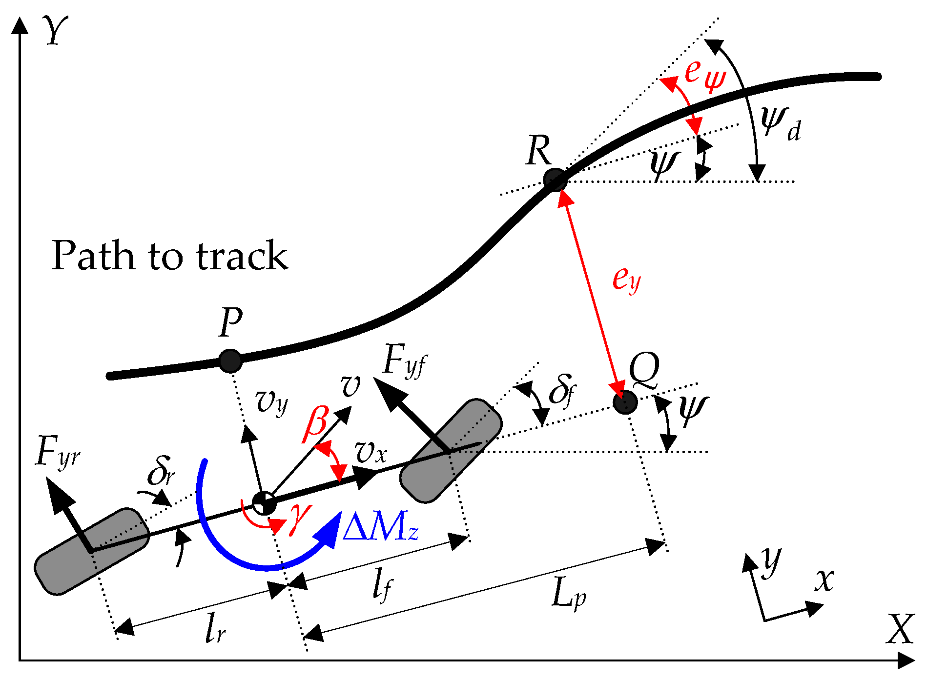
2.1. Derivation of State–Space Model

For path tracking, a 2-DOF bicycle model was chosen as the vehicle model, as discussed in the literature [12,14,15,16,17,18,19,20,21,22,23,24,25,26,28,30,33,35,36,37,38,48]. Figure 2 outlines the coordinates, geometry, and the parameters of the 2-DOF bicycle model. This model assumes that the longitudinal velocity (vx) is constant [49,50]. The state variables in the model are γ and β. The equations of motion (1) are established from the free-body diagram in Figure 2 [17,36,37,38,48]. The slip angles, θf and θr, are calculated in (2) at the front and rear wheels, and the lateral tire forces, Fyf and Fyr, are calculated in (3), assuming that they are linear. From (1), (2), and (3), the linear state–space model is derived in (4).
m v x β ˙ + γ = F y f + F y r I z γ ˙ = l f F y f l r F y r + Δ M z
θ f = δ f tan 1 β + l f γ v x δ f β l f γ v x θ r = δ r tan 1 β l r γ v x δ r β + l r γ v x
F y f = C f θ f , F y r = C r θ r
β ˙ = ς 1 m v x β + ς 2 m v x 2 1 γ + C f m v x δ f + C r m v x δ r γ ˙ = ς 2 I z β + ς 3 I z v x γ + l C f f I z δ f l C r r I z δ r + Δ M z I z ς 1 = C f C r , ς 2 = C f l f + C r l r , ς 3 = l f 2 C f l r 2 C r
Most of papers in the literature on path tracking have defined and used ey and eψ at point C, the vehicle’s CoG, as depicted in Figure 2. To improve the performance of path tracking, a preview function has been adopted, as proposed in previous studies [12,13,17,21,22,28,36,37,38]. The preview distance, Lp, is defined in (5), where kv is the velocity gain. In the previous work, without a preview function, the target heading angle is determined at point P. Different from the previous work, the preview point, Q, and point R on the target path are determined by using the preview distance, Lp, as shown in Figure 2. At point R, the target heading angle is defined as ψd. With the target heading angle and the heading one at point R, eψ is defined as the difference between them. Moreover, at point R, ey is also defined [12,13,21,22,28]. The derivatives of both ey and eψ are calculated, as described in (6), assuming eψ is small, at less than 15°. In (6), χ is the curvature of the target path at point R, which acts as a disturbance.
L p = k v v x
e ˙ y = v x sin ( e ψ ) v x β L p γ v x e ψ v x β L p γ e ˙ ψ = ψ ˙ d ψ ˙ = v x χ γ
With the state variables ey, eψ, β, and γ, the state vector, x, the disturbance, w, and control input u are defined in (7) [36,37,38]. By combining (4), (6) and (7), the state–space model for path tracking is obtained in (8), where the matrices A, B1, and B2 are given in (9). As shown in A and B2, it is assumed that vx is constant, which is not realistic. Moreover, the preview distance, Lp, in A is time-varying because it depends on vx. As a consequence, the state–space equation of (8) is uncertain and time-varying in real situations. To cope with the variation in Lp, an adaptive preview distance scheme was proposed in previous work [38]. The effects of the measurement error and noise in ey and eψ on the path tracking performance were analyzed in reference [9]. Robust control methodologies, such as guaranteed cost control or quadratic stabilization, can be applied to cope with uncertain and time-varying parameters in A and B2. However, this is out of scope in this paper.
x = e y e ψ β γ T , w = χ , u = δ f δ r Δ M z T
x ˙ = A x + B 1 w + B u 2
A = 0 v x v x L p 0 0 0 1 0 0 ς 1 m v x ς 2 m v x 2 1 0 0 ς 2 I z ς 3 I z v x , B 1 = 0 v x 0 0 , B 2 = 0 0 0 0 0 0 C f m v x C r m v x 0 l C f f I z l C r r I z 1 I z
The vector of the control inputs, u, in (7) consists of three elements: δf, δr, and ΔMz. These elements are used to define three distinct vectors of the control inputs, u1, u2, and u3, which correspond to the input configurations, IPC#1, IPC#2, and IPC#3, as given in references [36,37]. Derived from (9), the input matrices B21, B22, and B23 are determined in (10), where the matrix B2,k represents the k-th column of B2 in (9). In the case of IPC#3, ΔMz is generated by RWS, 4WIB, 4WID, and its seven combinations, i.e., RWS, 4WIB, 4WID, 4WIB+4WID, RWS+4WIB, RWS+4WID, and RWS+4WIB+4WID. For this reason, it is necessary to convert ΔMz into the rear steering angle, δr, and the braking and tractive torque, TBi and TDi, at each wheel. In this paper, TBi and TDi at wheel i are generated by 4WIB and 4WID, respectively.
u 1 = δ f B 21 = B 2 , 1 for I P C # 1 u 2 = δ f δ r T B 22 = B 2 , 1 B 2 , 2 for I P C # 2 u 3 = δ f Δ M z T B 23 = B 2 , 1 B 2 , 3 for I P C # 3

2.2. Design of LQR for Path Tracking

In the case of designing the LQR, an LQ cost function should be defined. The input configurations IPC#1, IPC#2, and IPC#3 have associated LQ cost functions, denoted as J1, J2, and J3, which are given in (11). These can be transformed into a vector–matrix form, as given in (12). The weighting matrices Q and Ri in (12) can be derived from (11), as given in (13). The weight, ρi, is determined through Bryson’s rule, as outlined in (14), where ξi represents the maximum allowable value (MAV) for the respective term [17,36,37,38,51]. By adjusting ξi, the path tracking performance can be tuned. For IPC#i, the control input, ui, of the LQR is calculated using formula (15), where Pi is the solution to the Riccati equation for IPC#i.
J 0 = 0 ρ 1 e y 2 + ρ 2 e φ 2 + ρ 3 β 2 + ρ 4 γ 2 d t J 1 = J 0 + 0 ρ 5 δ f 2 d t for I P C # 1 J 2 = J 0 + 0 ρ 5 δ f 2 + ρ 6 δ r 2 d t for I P C # 2 J 3 = J 0 + 0 ρ 5 δ f 2 + ρ 7 Δ M z 2 d t for I P C # 3
J i = = 0 x u i T Q 0 0 R i x u i d t , i = 1 , 2 , 3
Q = d i a g ρ 1 , ρ 2 , ρ 3 , ρ 4 , R 1 = ρ 5 for I P C # 1 R 2 = d i a g ρ 5 , ρ 6 for I P C # 2 R 3 = d i a g ρ 5 , ρ 7 for I P C # 3
ρ i = 1 ξ i 2
u i = K i x = R i 1 B 2 i T P i x , i = 1 , 2 , 3

2.3. Design of LQ SOF Controllers for Path Tracking

The sensor outputs for the SOF controller are defined in (16). As shown in (16), the vectors of sensor outputs, y2 and y3, use the lateral offset, heading errors, and yaw rate, respectively. The vectors, y2 and y3, have been used in previous works [44,47]. Using these vectors, the SOF controllers are defined in (17).
y 2 = e y e ψ = 1 0 0 0 0 1 0 0 x = C 2 x y 3 = e y e ψ γ = 1 0 0 0 0 1 0 0 0 0 0 1 x = C 3 x
u r , i = K r y r = K r C r x , i = 1 , 2 , 3 , r = 2 , 3
It is known that there are no analytical methods to find the optimal gain matrices K2 and K3 for the SOF controllers, which minimize the LQ cost functions [39]. For this reason, the optimization problem is formulated to find the K2 and K3, as in (18). In (18), Kr is either K2 or K3. The second row of the constraints in (18) means that the closed-loop system should be stable for the given Kr. The optimization problem (18) is known as non-convex, where a global optimum cannot be guaranteed [39]. To solve this problem, meta-heuristic methods, such as the genetic algorithm (GA), the evolutionary strategy (ES), and particle swarm optimization (PSO), have been proposed and successfully applied to date [52,53]. Among them, a meta-heuristic method, CMS-ES, is applied in this paper [54]. A detailed description of CMA-ES can be found in references [54,55]. Let the resulting SOF controllers using y2 and y3 from (18) be denoted as LQSOF2 and LQSOF3, respectively.
min K r J i = trace P i s . t . P i = P i T > 0 max Re A + B 2 i K r C r < 0 A + B 2 i K r C r T P i + P i A + B 2 i K r C r + Q + C r T K r T N i T + N i K r C r + C r T K r T R i K r C r = 0 i = 1 , 2 , 3 r = 2 , 3

2.4. Design of SOF SMC

To date, the SMC has been designed with a full-state feedback structure for path tracking [17,21]. With the vectors of outputs, y2 and y3, the SOF SMC is designed in this paper. The SMC also uses the state–space model (8). The sliding surface or error surface, s, to be minimized is defined in (19), where M is the matrix representing the weights on the state variables. Note that s is scalar. Generally, M is set to the row vector corresponding to the state vector, x. The convergence condition of the sliding surface is given in (20). In (20), KSMC is a parameter that is used to tune the convergence speed of s. Naturally, the larger the KSMC, the faster the convergence speed of s. By combining (19), (20) and (8), (21) is obtained. From (21), the control input of the full-state feedback SMC is derived in (22) [17,21]. In (22), (•)+ is the pseudo-inverse of a matrix (•). In this paper, the disturbance feedforward term, i.e., the second term on the right side of (22), is neglected. The design parameters of the SMC are M and KSMC.
s = M x
s ˙ = K S M C s K S M C > 0
s ˙ = M x ˙ = M A x + B 1 w + B u i 2 i = K S M C M x , i = 1 , 2
u i = M B 2 i + M A + K S M C I x M B 2 i + M B 1 w , i = 1 , 2
When designing the SMC for IPC#3, ΔMz is included in the control input, u3. In u3, there are large differences between the gains for FWS and ΔMz. For this reason, the control inputs, u1 and u3, for FWS and ΔMz, are separately designed, as given in (23) and (24), if IPC#3 is selected. Then, these control inputs are combined into u3, as given in (25).
s ˙ = M x ˙ = M A x + B 1 w + B u i 2 , i = K S M C M x , i = 1 , 3
u i = M B 2 , i + M A + K S M C I x M B 2 , i + M B 1 w , i = 1 , 3
u 3 = u 1 u 3 = M B 2 , 1 + M A + K S M C I M B 2 , 3 + M A + K S M C I x
In (22) and (25), the SMC has the full-state feedback form. For this reason, it should be transformed into the SOF form. By combining (17) with (22) or (25), (26) is obtained. By comparing the coefficients of both sides in (26), (27) is obtained. From (27), the gain matrix of the SOF SMC is obtained in (28). Let the resulting SOF controllers using y2 and y3 from (28) be denoted as the SOFSMC2 and SOFSMC3, respectively.
u i , r = K r y r = K r C r x = M B 2 + M A + K S M C I x , i = 1 , 2 , 3 , r = 2 , 3
K r C r = M B 2 i + M A + K S M C I , i = 1 , 2 , 3 , r = 2 , 3
K r = M B 2 i + M A + K S M C M C r + , i = 1 , 2 , 3 , r = 2 , 3

2.5. Constraints Related to Tire Slip Angle

In previous work, the constraints related to the tire slip angle were proposed to avoid the saturation of lateral tire force, Fy [37]. Fyf and Fyr are easily saturated by excessive steering as θ goes over θm, which is a value that gives the maximum Fy. As a result, as Fy decreases, path tracking performance deteriorates. The idea of the constraints related to the tire slip angle is simple, where δf and δr are constrained such that θ cannot exceed θm.
It is assumed that Fy has its maximum, Fy,max, at the tire slip angle θm. If θ is larger than θm, Fy is saturated and smaller than Fy,max [49,50]. In the case of this condition, a path tracking controller cannot provide the maximum performance. For this reason, θ should be constrained to be smaller than θmax, as given in (29). θmax is not necessarily identical to θm, where θm is determined by a particular tire model or carpet plot data, and θmax is set by a designer. By combining (29) with (2), (30) is derived. From (30), the constraints on δf and δr are obtained in (31). The constraints, (31), are applied to the steering angles obtained from the LQR, LQ SOF controller, and SOF SMC. In previous work, θmax was set to 5°.
As shown in (31), it is essential to measure or estimate β. However, it is hard to measure β with an onboard sensor in real vehicles. Moreover, the SOF controllers presented in (17) do not use β. For this reason, (31) cannot be used for the SOF controllers. However, from the experiences in the simulations, the front steering angles did not go over 8° on low-μ surfaces [17,36,37,38]. Following this fact, δf and δr are constrained, as in (32), where σmax is the maximum steering angle used to avoid the saturation of the lateral tire forces [37].
θ θ m a x
θ f = δ f β l f γ v x θ m a x , θ r = δ r β + l r γ v x θ m a x
θ m a x + β + l f γ v x δ f θ m a x + β + l f γ v x θ m a x + β l r γ v x δ r θ m a x + β l r γ v x
σ m a x δ f , δ r σ m a x

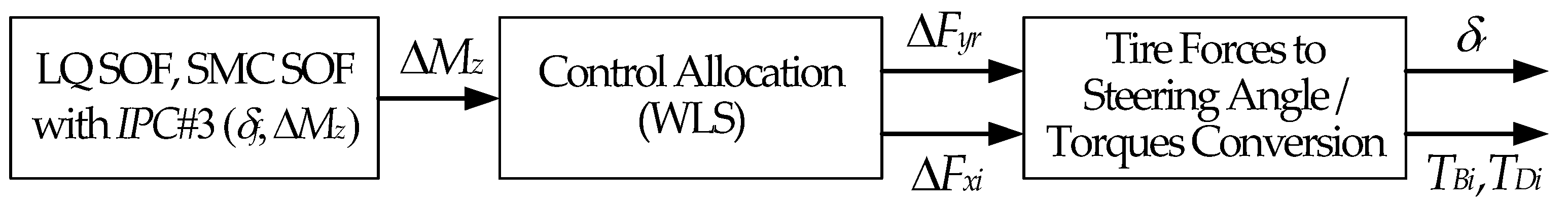
2.6. Control Allocation for LQR, LQ SOF Controllers, and SOF SMC

In accordance with (10), ΔMz is derived from IPC#3. After the controller obtains ΔMz, it should be transformed into additives, ΔFx and ΔFy, acting on the wheels. These forces are generated by seven actuator combinations consisting of RWS, 4WIB, and 4WID. Typically, this is accomplished by control allocation [15,17,20,21,22,23,24,28,29,33,35,36,37,38,44,47]. Following previous work, a weighted least squares-based method is employed for control allocation in this paper [20,21,23,29,35,44]. After obtaining the ΔFx and ΔFy acting on the wheels, they are transformed into the rear steering angle and braking and driving torques of the wheels. Figure 3 summarizes this procedure.
Figure 4 illustrates the geometric relationship among the tire forces, ΔFyr, ΔFx1, ΔFx2, ΔFx3, ΔFx4, and ΔMz, when ΔMz is positive [36,37,38]. In Figure 4, the wheel indices are 1, 2, 3, and 4, in order from the front left, front right, rear left, and rear right wheels, respectively. Within Figure 4, ΔFyr is generated by RWS. ΔFx1, ΔFx2, ΔFx3, and ΔFx4 are generated by 4WIB and 4WID. According to the sign of ΔFxi, it corresponds to the tractive torque TDi generated by 4WID or the braking torque TBi generated by 4WIB. These five tire forces need to be determined to generate ΔMz, and the weighted least squares (WLSs)-based method is utilized for this purpose.
The vectors for the five tire forces to generate ΔMz are shown in Figure 4, as expressed in (33) [36,37,38]. The components of vector z are given in (34).
c 1 c 2 c 3 c 4 c 5 z Δ F y r Δ F x 1 Δ F x 2 Δ F x 3 Δ F x 4 q = Δ M z
c 1 = 2 l r cos δ r , c 2 = l f sin δ f + 0.5 t f cos δ f , c 3 = l f sin δ f 0.5 t f cos δ f , c 4 = l r sin δ r + 0.5 t r cos δ r , c 5 = l r sin δ r 0.5 t r cos δ r
The quadratic form defines the cost function for weighted least squares, as in (35). In (35), ζi is the product of μ and Fzi at wheel i, i.e., μFzi, which represents the friction circle radius. In (35), the radii of the friction circles, μFzi, must be estimated. For the purpose of this paper, Fzi is estimated using longitudinal and lateral accelerations [56]. In addition to this, μ is assumed to be estimated using the observer proposed in reference [57]. The vector of virtual weights, denoted as κ, is introduced in (35) for the purpose of selecting the combination of actuators [36,37,38]. The equality constraint (33) is transformed into a quadratic form, as shown in (36). In previous research, the satisfaction of (33) was essential for generating ΔMz. The cost function (35) and the constraint (36) are unified into a single cost function (37) through the utilization of the Lagrange multiplier, η. In (37), it is imperative to set η to a value of 1 or higher; otherwise, the constraint (36) will not be met. The optimal solution for (37) is algebraically derived in (38) by taking the derivative of (37) with respect to q [36,37,38].
J Q = κ 2 Δ F x 1 2 ζ 1 2 + κ 3 Δ F x 2 2 ζ 2 2 + κ 1 Δ F y r 2 + κ 4 Δ F x 3 2 ζ 3 2 + κ 1 Δ F y r 2 + κ 5 Δ F x 4 2 ζ 4 2 = q T Θ q Θ = diag 1 ζ 3 2 + 1 ζ 4 2 , 1 ζ 1 2 , 1 ζ 2 2 , 1 ζ 3 2 , 1 ζ 4 2 κ κ = diag κ 1 κ 2 κ 3 κ 4 κ 5
J E C = z q Δ M z T z q Δ M z
J C A = J Q + η J E C = q T Θ q + η z q Δ M z T z q Δ M z
q o p t = η Θ + η z T z 1 z T Δ M z
When the weighted least squares are applied to the control allocations involving ΔMz, an arbitrary combination of actuators comprising RWS, 4WIB, and 4WID can be configured based on a specific input configuration. To account for this variability, the virtual weights, denoted as κi, can be customized to match a particular combination selected from RWS, 4WIB, 4WID, 4WIB+4WID, RWS+4WIB, RWS+4WID, and RWS+4WIB+4WID [36,37,38]. The vectors of the virtual weights regarding RWS are outlined in (39). Initially, all the virtual weights are set to 1. In (39), the value of ε is 10−4, and the terms marked with • insignificantly impact the steering actuator. The first term of κ in (39) corresponds to ΔFyr, which is converted into δr. When the first term of κ is adjusted to ε, ΔFyr is generated through the weighted least squares process, as depicted in the first row of (39).
RWS :       κ = diag ε No RWS : κ = diag 1
The vectors of the virtual weights regarding 4WIB and 4WID are provided in (40). As depicted in Figure 4, it becomes evident that only ΔFx2 and ΔFx4 should be generated in the event of a negative ΔMz and the availability of 4WIB. This scenario is illustrated by the second row of the first term, 4WID, in (40). If both 4WIB and 4WID are accessible for ΔMz generation, no restrictions are imposed on ΔFx’s, as indicated in the last row in (40). The virtual weights, as presented in (39) and (40), can be configured in accordance with the available combinations of actuators, RWS, 4WIB, 4WID, 4WIB+4WID, RWS+4WIB, RWS+4WID, and RWS+4WIB+4WID, intended for ΔMz generation.
4 WID : κ = diag 1 ε 1 ε if Δ M z > 0 κ = diag ε 1 ε 1 if Δ M z < 0 4 WIB : κ = diag ε 1 ε 1 if Δ M z > 0 κ = diag 1 ε 1 ε if Δ M z < 0 4 WID / 4 WIB : κ = diag ε ε ε ε
The sets of virtual weights corresponding to actuator combinations in IPC#3 are summarized in Table 1. As shown in Table 1, seven actuator combinations, AC#3, …, AC#8 and AC#9 in IPC#3, are selected by setting the vector of the virtual weights. For example, AC#6 or (FWS+RWS+4WID+4WIB) can be selected by setting κ to diag[ε ε ε ε ε].
In this paper, TBi and TDi for wheel i are computed based on the values of ΔFx1, ΔFx2, ΔFx3, and ΔFx4, which are determined through the weighted least squares-based method, specifically utilizing qopt, as presented in (41). Depending on the sign of ΔFxi, the calculations for TBi and TDi at wheel i are carried out as in (41), respectively [36,37,38].
T B i if Δ F x i < 0 T D i if Δ F x i > 0 = h r w i Δ F x i υ i , ω i , i = 1 , , 4
The calculation of δr is performed by utilizing the value of ΔFyr, acquired from qopt and the definitions found in (2) and (3). ΔFyr is transformed into the rear slip angle, θr, using the second term in (3). Through the utilization of (2), δr is subsequently determined, as outlined in (42) [45]. The SOF controllers using y2 and y3 cannot use β. For this reason, (43) is used instead of (42).
δ r = α r + β l r γ v x Δ F y r 2 C r + β l r γ v x
δ r Δ F y r 2 C r l r γ v x

3. Performance Evaluation for Path Tracking Control

In the domain of path tracking, ey and eψ have traditionally served as measures for assessing path tracking performance. Different from these measures, recent papers have proposed other measures by adopting a double lane change maneuver for collision avoidance as the target path [11,16,17,19,20,26,27,29,30,32,38,47]. This path is selected to assess the reachability and agility of path tracking [17,36,37,38]. Figure 5 presents the path to track and the actual trajectory of the vehicle. Five metrics, from D1 to D4 and DOS, are defined in (44), based on the points, from P1 to P3, on the path, and from A1 to A4 on the actual trajectory, as shown in Figure 5. In (44), D1 and D2 stand for the longitudinal and lateral offsets of the peak, respectively. D3 and D4 can be considered as the response delay and settling delay, both of which have units of meters, respectively. DOS is a measure of how much overshoot occurred. In (44), x and y, in the parentheses, correspond to the x- and y-positions of point •, respectively. Naturally, the smaller these metrics, the better the path tracking performance, except for D2.
D 1 = x A 1 x P 1 = x A 1 73.2 D 2 = y A 1 y P 1 = y A 1 3.53 D 3 = x A 2 x P 2 = x A 2 91.5 D 4 = x A 4 x P 3 = x A 4 190.0 D O S = y A 3 1.65 1.65 + 3.53 × 100
In Figure 5, the agility and reachability of the controller are measured by D1 and D2, respectively. In this paper, if D2 exceeds −0.05 m, the controller’s path tracking performance is regarded as satisfactory. DOS indicates the lateral damping capability, standing for its agility. In this paper, the performance is satisfactory if DOS remains below 16%. D3 represents the response delay, standing for the agility along the longitudinal motion. D4 can be interpreted as the settling time in transient responses, or the settling distance needed to converge to A4, indicating the convergence speed of the vehicle’s lateral motion toward the target y-position, i.e., −1.65 m. In this research, the performance is regarded as satisfactory if D4 is less than 16 m on low-friction surfaces. Generally, the best performance is attained when DOS is around 1%, provided that D2 exceeds −0.05 m. In this paper, the weights and kv in J1, J2, and J3 are tuned such that D2 is maintained near −0.02 m. In this case, DOS is always less than 1%. More comprehensive explanations of these measures can be found in references [17,36,37,38].
Generally, lateral stability is represented by β. In a real vehicle, it is regarded that lateral stability is maintained if β is controlled not to exceed 3° [36]. Generally, the smaller the β, the better. In this paper, let max β denote the maximum absolute value of β. In this way, the maximum absolute value of the angular rate of β is defined as max β ˙ .

4. Simulation and Discussion

To verify the effects of the SOF controllers and input configurations on path tracking performance, simulations were performed. The six path tracking controllers, i.e., two full-state feedback controllers, i.e., a full-state feedback LQR and a full-state feedback SMC, and four SOF controllers, i.e., LQSOF2, LQSOF3, SOFSMC2, and SOFSMC3, were implemented with MATLAB/Simulink 2019a, connected to CarSim 8.0 [58]. The test scenario was given in Figure 5. As a test vehicle, the F-segment sedan model in CarSim was selected [17,36,37,38]. This model is a nonlinear 27-DOF model with a single sprung mass, four wheels, suspensions, and a steering mechanism. In the model, nonlinear tire models, represented by a carpet plot, were used. The spring and the damper in this model are nonlinear, represented by piece-wise linear interpolation [56]. The parameters of the F-segment sedan are given in Table 2.
In this paper, it was assumed that the target vehicle had the actuators, FWS, RWS, 4WIB, and 4WID, which were modeled as a first-order system. The bandwidths for the steering actuators were set to 5 Hz, and the bandwidths for 4WIB and 4WID were set to 2 Hz, respectively. The initial speed was set to 60 km/h, which was maintained as a constant using a built-in speed controller provided in CarSim. The simulations were performed on high- and low-friction surfaces, where μ was 0.8 and 0.5, respectively. In this paper, speed variation is not considered because the path tracking performance of a controller at low speeds is better than that at high speeds. The simulation horizon was set to 10 s.
As pointed out in previous work, ΔMz should be limited to a smaller δr and β. From the maximum lateral tire forces and geometric information from CarSim, it was limited to 11,400 Nm [36]. When using full-state feedback controllers, θmax was set to 5°, which was obtained from CarSim tire data. When using the SOF controllers, σmax was set to 8°.
In the simulations, the weights in the LQ cost function, the gain of the SMC, and the preview distance were tuned for each controller and actuator combination until a satisfactory result was obtained. For this reason, the tuning parameters are different from one another, according to the selected controller and the actuator combination.
In the simulations, the LQR and SMC are used as a baseline. The other path tracking controllers, such as the pure pursuit method, Stanley method, PID control, LQR, MPC, and SMC, were compared, as in previous work [9,17]. As mentioned earlier, it is impossible to use MPC with an SOF control because the initial state variables for MPC cannot be obtained using SOF. Moreover, it was shown that the path tracking performance of the MPC is nearly identical to that of the LQR [17].

4.1. Simulation on High-Friction Surfaces

The first simulation was performed for six controllers on the road where μ was 0.8. The velocity gain, kv, was set to 0.18. The weights in the LQ cost function were tuned such that D2 was near −0.020 m and max β was less than 2°. As a result, D2 and DOS can be neglected because they were nearly identical values over several actuator combinations.
Table 3, Table 4, Table 5, Table 6, Table 7 and Table 8 show the simulation results for the LQR, LQSOF2, LQSOF3, SMC, SOFSMC2, and SOFSMC3, respectively. In these tables, AC#1, …, AC#8, and AC#9 in the second column represent the actuator combinations, FWS, 4WS, FWS+RWS, FWS+RWS+4WID, FWS+RWS+4WIB, FWS+RWS+4WID+4WIB, FWS+4WID, FWS+4WIB, and FWS+4WIB+4WID, respectively.
In terms of the LQOC, including the LQR and LQ SOF controllers, as given in Table 3, Table 4 and Table 5, the LQSOF2 is better than the LQR in terms of D1 and D3, and the LQSOF3 is better than the LQR in terms of D3 and D4. Moreover, when the LQSOF2 is applied, D1 and max β are inversely proportional to each other, as given in Table 4. A notable feature of the LQSOF2 is that it gives the smallest D1 and the largest max β among the three controllers. This is caused by the fact that β is not used in the LQSOF2. On the contrary, this fact does not hold for the LQR and LQSOF3. Compared to the LQSOF2, there are few differences between the LQR and LQSOF3. For this reason, the LQSOF2 is preferred over the LQSOF3. In other words, if the yaw rate, γ, is used for the LQSOF3, it shows a nearly identical performance to the LQR. For LQR, AC#7 is the best actuator combination. For LQSOF2, AC#1, AC#7, and AC#8 show the best performances. For the LQSOF3, AC#5 is the best actuator combination. These facts can be identified in Table 3, Table 4 and Table 5.
In view of the SMC, SOFSMC2 and SOFSMC3 are better than the SMC in terms of D1. On the contrary, there are few differences among the SMC, SOFSMC2, and SOFSMC3 in terms of D3 and D4. Similar to the LQSOF2, the SMCSOF2 gives the smallest D1 and the largest max β among the three controllers, and D1 and max β are inversely proportional to each other when using the SMCSOF2, as given in Table 7. This is caused by the fact that β is not used in the SMCSOF2. On the contrary, if the yaw rate, γ, is used for the SMCSOF3, it shows nearly identical performance to the SMC. For the SMC, AC#1 is the best actuator combination. For the SMCSOF2, AC#5 shows the best performance. For SMCSOF3, AC#8 is the best actuator combination.
As shown in Table 3, Table 4, Table 5, Table 6, Table 7 and Table 8, there are slight differences among the nine actuator combinations, AC#1, …, AC#8, and AC#9, given in IPC#1, IPC#2, and IPC#3 for a single controller. This is a natural consequence, as each tire can generate larger forces on high-friction surfaces. These results mean that the simplest actuator, i.e., AC#1, FWS, is recommended on high-friction surfaces. If collision avoidance is critical, then the LQSOF2 and SOFSMC2 are recommended because they give the smallest D1.
Figure 6 and Figure 7 show the simulation results for the LQSOF2 and SOFSMC2 for each actuator combination on high-friction surface. As shown in Figure 6 and Figure 7, there are few differences in vehicle trajectories and heading angles with the LQSOF2 and SMCSOF2 for the nine actuator combinations, AC#1, …, AC#8, and AC#9. This is caused by the fact that path tracking controllers show good performance on high-friction surfaces, regardless of controller design methodologies or control structures, and that the tuning parameters of the LQSOF and SOFSMC were finely tuned for each actuator combination. In other words, D1 and DOS were tuned to show nearly identical values to one another for actuator combinations, which resulted in nearly the same responses.

4.2. Simulation on Low-Friction Surfaces

The second simulation was performed for six controllers on the road, where μ was 0.4. The velocity gain, kv, was set to 0.25. The weights in the LQ cost function were tuned such that D2 was near −0.020 m and max β was less than 2°. As a result, D2 and DOS can be neglected because they were nearly identical values over several actuator combinations.
Table 9, Table 10, Table 11, Table 12 and Table 13 show the simulation results for the LQR, LQSOF3, SMC, SOFSMC2, and SOFSMC3, respectively. In the simulation, for the LQSOF2, it was impossible to find a controller gain that gave a convergent trajectory. In other words, it is not recommended that the LQ SOF control using (ey, eψ) be used for path tracking on low-friction surfaces. As shown in this case, the deviation between the controllers increases on low-friction surfaces. In these results, the LQR and SMC are used as a baseline.
Table 9 and Table 10 show the simulation results for the LQR and LQSOF3, respectively. As shown in these tables, the LQSOF3 shows slightly worse performance than the LQR. For example, the D1, D3, and D4 for the LQSOF3 were slightly increased, compared to those for the LQR. The D3 of the LQR varies from 7.90 to 8.91, while the D3 of the LQSOF3 varies from 8.52 to 10.35. The D4 of the LQR varies from 3.89 to 5.23 while the D3 of the LQSOF3 varies from 3.67 to 7.51. This is caused by the fact that β is not used for control. For this reason, the LQR is preferred over the LQSOF3 on low-friction surfaces. In view of the actuator combination, AC#2 and AC#3 show the best performance for the LQR, and AC#3 and AC#5 show the best performance for the LQSOF3.
Table 11, Table 12 and Table 13 show the simulation results for the SMC, SOFSMC2, and SOFSMC3, respectively. As shown in these tables, the SOFSMC2 outperforms the SMC and SOFSMC3 in terms of path tracking performance. Moreover, the SOFSMC2 outperforms the LQR. On the other hand, the SMC and SMCSOF3 show almost the same results as each other. In other words, if the yaw rate, γ, is used for the SMCSOF3, it shows nearly identical performance to the SMC. For this reason, the SMCSOF2 is preferred over the SMC and SMCSOF3 on low-friction surfaces.
In view of the actuator combination, the best actuator combinations for the SMC, SOFSMC2, and SOFSMC3 are AC#8, AC#5, and AC#8, respectively. From those results, it is recommended to use the SOFSMC2 using (ey, eψ) on low-friction surfaces and to select the actuator combination AC#8.
Figure 8 and Figure 9 show the simulation results for the LQSOF3 and SOFSMC3 for each actuator combination on low-friction surfaces. As shown in Figure 8 and Figure 9, there are few differences in vehicle trajectories and heading angles for the LQSOF3 and SMCSOF3 using the actuator combinations in spite of low-friction surfaces. It is natural that every actuator combination is tuned to give the best result. In other words, D1 and DOS were tuned to show nearly identical values to one another for actuator combinations, which resulted in nearly the same responses.

4.3. Discussion on Simulation Results

In Section 4.1 and Section 4.2, the proposed LQ SOF and SOF SMC controllers were verified through simulations using the vehicle simulation package. As a result, it was shown that both SOF controllers are effective in path tracking with multiple actuators. When implementing those controllers, there are obstacles, such as uncertain and time-varying parameters, measurement error, and noise. The most critical problem is to tune the velocity gain, kv, according to the tire–road friction. This was investigated in reference [38]. Another problem in the real-world implementation of these controllers is caused by parameter uncertainties, measurement error, and noise. The parameter uncertainty can be overcome by using a robust controller [5,6,8,9]. The measurement noise can be cancelled by a filter, which causes a delay in the output signals. The delay caused by a filter can severely deteriorate path tracking performance [8,9,59]. The last implementation issue is caused by controller fragility. The controller fragility of the LQ SOF and SOF SMC controllers presented in this paper can deteriorate path tracking performance. To date, there have been few approaches for non-fragile path tracking control. In the area of robot trajectory tracking control, a robust non-fragile controller has been designed [60,61].

5. Conclusions

This paper presented a method for designing a path tracking controller using a static output feedback control structure. From a 2-DOF bicycle model and a target path, a state–space model was derived. In the state–space model, three input configurations, representing nine actuator combinations, were defined. With the state-space model, the LQ cost functions, full-state feedback LQR, and full-state feedback SMC were designed. Two sets of sensor outputs were defined for the SOF control. Using these sets, the LQ SOF and SOF SMC controllers were designed by using LQOC and SMC methodology. To distribute ΔMz in IPC#3, the weighted least squares-based method was applied as a control allocation. To maximize the performance, the constraints related to the tire slip angle were imposed on the steering angles. To verify the performance of the path tracking controllers using the SOF control structure, simulations were performed in the vehicle simulation package, CarSim. From the simulation results, the following points were identified:
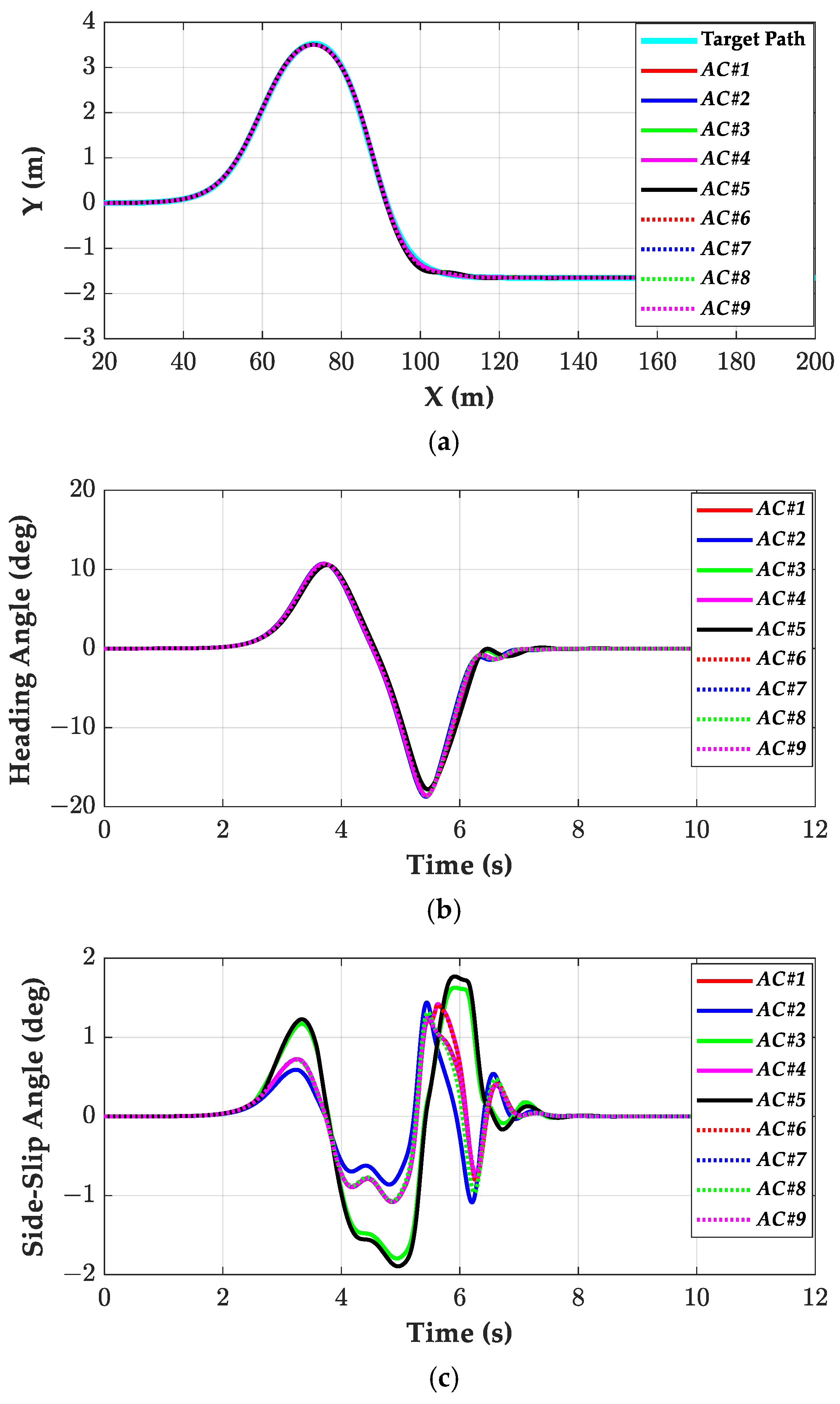
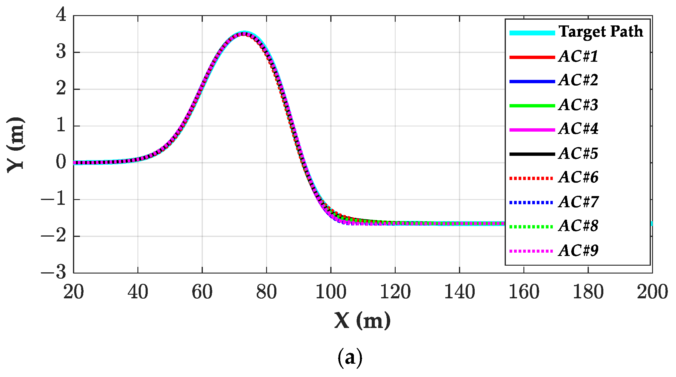
  • The LQ SOF and SOF SMC controllers, using three sensor outputs, can give equivalent performances as the full-state feedback controls, LQR, and SMC. In other words, the LQ SOF and SOF SMC show nearly identical performance to the LQR and SMC if the yaw rate is used for the control, respectively. On the contrary, the SOF controllers using two sensor signals show the smallest D1 and the largest side-slip angle because the side-slip angle is not used in the control. From the simulation results, small differences in terms of path tracking performance can be identified. This means that the side-slip angle and the yaw-rate signals are not needed for path tracking. In other words, the LQ SOF and SOF SMC controllers with two sensor signals, i.e., the LQSOF2 and SMCSOF2, are recommended for path tracking.
  • In view of the actuator combination, it was shown that there are small differences among actuator combinations derived from three input configurations. This is caused by the fact that each tire can generate a larger lateral force on high-friction surfaces, and that each tire can generate a very small lateral force on low-friction surfaces. On high-friction surfaces, the simplest actuator, i.e., FWS, is recommended among the actuator combinations. If collision avoidance is critical, then the LQSOF2 and SOFSMC2 are recommended because they can reduce D1. On low-friction surfaces, IPC#3 (FWS+RWS) is recommended for the LQR and LQSOF3, and IPC#3 (FWS+4WIB) is recommended for the SOFSMC2.
Based on the above results, it is desirable to use the LQSOF2 or SMCSOF2 with the actuator combinations FWS, FWS+RWS, or FWS+4WIB. Among the three actuator combinations, the third is preferred because 4WIB is mandatory to be installed on a real vehicle.
As mentioned earlier, parameter uncertainty, measurement error, and noise can deteriorate path tracking performance. Moreover, the controller gains of the LQ SOF and SOF SMC controllers are sensitive to their variations. To cope with these problems, a robust and non-fragile controller will be designed in future research.

Author Contributions

Conceptualization, M.P. and S.Y.; methodology, S.Y.; software, M.P.; validation, M.P. and S.Y.; formal analysis, S.Y.; investigation, M.P.; resources, M.P.; data curation, S.Y.; writing—original draft preparation, S.Y.; writing—review and editing, M.P.; visualization, S.Y.; supervision, M.P.; project administration, M.P.; funding acquisition, M.P. All authors have read and agreed to the published version of the manuscript.

Funding

This work was supported by the Ministry of Trade, Industry and Energy (MOTIE, Republic of Korea). [Project Name: Development of Fail Operation Technology in Lv.4 Autonomous Driving Systems/ Project Number: 20018055]. This work was supported by the Ministry of Trade, Industry, and Energy (MOTIE, Republic of Korea). [Project Name: Development of Demand-Responsive Automatic Parking and Service Technology/Project Number: 20018448].

Data Availability Statement

The original contributions presented in this study are included in the article. Further inquiries can be directed to the corresponding author.

Conflicts of Interest

The authors declare no conflicts of interest.

Abbreviations

The following abbreviations are used in this manuscript:
4WIBfour-wheel independent braking
4WIDfour-wheel independent driving
4WSfour-wheel steer = FWS + RWS
CoGcenter of gravity
ESCelectronic stability control
EVelectric vehicle
FWSfront wheel steering
IPCinput configuration
LQOClinear quadratic optimal control
LQRlinear quadratic regulator
LSClateral stability control
MPCmodel predictive control
RWSrear wheel steering
SMCsliding mode control
SOFstatic output feedback
TVFtorque vectoring function
VSCvehicle stability control
WLSsweighted least squares
YRTyaw rate tracking
Nomenclature
Cf, Crcornering stiffness of front/rear tires (N/rad)
D1, D2longitudinal and lateral offsets (m)
D3, D4response and settling delays (m)
DOSpercentage overshoot
ey, eψlateral offset error (m) and heading error (rad)
Fyf, Fyrlateral tire forces of front and rear wheels (N)
Fzivertical tire force of wheel i (N)
ggravitational acceleration constant (=9.81 m/s2)
Izyaw moment of inertia (kg·m2)
kvvelocity gain or preview period in the lookahead distance (s)
Lplookahead or preview distance (m)
lf, lrdistance from C.G. to front and rear axles (m)
mvehicle total mass (kg)
vvehicle speed (m/s)
vx, vylongitudinal and lateral velocities at CoG of a vehicle (m/s)
ylateral displacement (m) from the preview point to the target path
βside-slip angle (rad)
ΔFxicontrol longitudinal tire force of wheel i (N)
ΔFyrcontrol lateral tire force of rear wheels (N)
ΔMzcontrol yaw moment (N·m)
δf, δrfront and rear steering angles (rad)
εvery small value, 10−4
χcurvature (1/m)
κivirtual weight on i-th term in the objective function of control allocation
κvector of virtual weights
γyaw rate (rad/s)
ξimaximum allowable value (MAV) of weight in LQ objective function
μtire–road friction coefficient
ψheading angle (rad)
ψdtarget heading angle (rad)
ρiweight in LQ objective function
σmaxmaximum steering angle used to limit the lateral tire force (rad)
θf, θrtire slip angles of front and rear wheels (rad)
θmaxmaximum tire slip angle used to limit the lateral tire force (rad)

References

  1. Montanaro, U.; Dixit, S.; Fallaha, S.; Dianatib, M.; Stevensc, A.; Oxtobyd, D.; Mouzakitisd, A. Towards connected autonomous driving: Review of use-cases. Veh. Syst. Dyn. 2019, 57, 779–814. [Google Scholar] [CrossRef]
  2. Yurtsever, E.; Lambert, J.; Carballo, A.; Takeda, K. A survey of autonomous driving: Common practices and emerging technologies. IEEE Access. 2020, 8, 58443–58469. [Google Scholar] [CrossRef]
  3. Omeiza, D.; Webb, H.; Jirotka, M.; Kunze, M. Explanations in autonomous driving: A survey. IEEE Trans. Intell. Transp. Syst. 2022, 23, 10142–10162. [Google Scholar] [CrossRef]
  4. Paden, B.; Cap, M.; Yong, S.Z.; Yershov, D.; Frazzoli, E. A survey of motion planning and control techniques for self-driving urban vehicles. IEEE Trans. Intell. Veh. 2016, 1, 33–55. [Google Scholar] [CrossRef]
  5. Sorniotti, A.; Barber, P.; De Pinto, S. Path tracking for automated driving: A tutorial on control system formulations and ongoing research. In Automated Driving; Watzenig, D., Horn, M., Eds.; Springer: Cham, Switzerland, 2017. [Google Scholar]
  6. Amer, N.H.; Hudha, H.Z.K.; Kadir, Z.A. Modelling and control strategies in path tracking control for autonomous ground vehicles: A review of state of the art and challenges. J. Intell. Robot. Syst. 2017, 86, 225–254. [Google Scholar] [CrossRef]
  7. Bai, G.; Meng, Y.; Liu, L.; Luo, W.; Gu, Q.; Liu, L. Review and comparison of path tracking based on model predictive control. Electronics 2019, 8, 1077. [Google Scholar] [CrossRef]
  8. Yao, Q.; Tian, Y.; Wang, Q.; Wang, S. Control strategies on path tracking for autonomous vehicle: State of the art and future challenges. IEEE Access. 2020, 8, 161211–161222. [Google Scholar] [CrossRef]
  9. Rokonuzzaman, M.; Mohajer, N.; Nahavandi, S.; Mohamed, S. Review and performance evaluation of path tracking controllers of autonomous vehicles. IET Intell. Transp. Syst. 2021, 15, 646–670. [Google Scholar] [CrossRef]
  10. Stano, P.; Montanaro, U.; Tavernini, D.; Tufo, M.; Fiengo, G.; Novella, L.; Sorniotti, A. Model predictive path tracking control for automated road vehicles: A review. Annu. Rev. Control 2022, 55, 194–236. [Google Scholar] [CrossRef]
  11. Yakub, F.; Mori, Y. Comparative study of autonomous path-following vehicle control via model predictive control and linear quadratic control. Proc. Inst. Mech. Eng. Part D J. Automob. Eng. 2015, 229, 1695–1714. [Google Scholar] [CrossRef]
  12. Wang, R.; Yin, G.; Zhuang, J.; Zhang, N.; Chen, J. The path tracking of four-wheel steering autonomous vehicles via sliding mode control. In Proceedings of the 2016 IEEE Vehicle Power and Propulsion Conference (VPPC), Hangzhou, China, 17–20 October 2016. [Google Scholar]
  13. Lee, K.; Jeon, S.; Kim, H.; Kum, D. Optimal path tracking control of autonomous vehicle: Adaptive full-state linear quadratic gaussian (LQG) control. IEEE Access 2019, 7, 109120–109133. [Google Scholar] [CrossRef]
  14. Hang, P.; Chen, X. Path tracking control of 4-wheel steering autonomous ground vehicles based on linear parameter-varying system with experimental verification. Proc. Inst. Mech. Eng. Part I J. Syst. Control. Eng. 2021, 235, 411–423. [Google Scholar] [CrossRef]
  15. Barari, A.; Afshari, S.S.; Liang, X. Coordinated control for path-following of an autonomous four in-wheel motor drive electric vehicle. Proc. Inst. Mech. Eng. Part C J. Mech. Eng. Sci. 2022, 236, 6335–6346. [Google Scholar] [CrossRef] [PubMed]
  16. Du, Q.; Zhu, C.; Li, Q.; Tian, B.; Li, L. Optimal path tracking control for intelligent four-wheel steering vehicles based on MPC and state estimation. Proc. Inst. Mech. Eng. Part D J. Automob. Eng. 2022, 236, 1964–1976. [Google Scholar] [CrossRef]
  17. Lee, J.; Yim, S. comparative study of path tracking controllers on low friction roads for autonomous vehicles. Machines 2023, 11, 403. [Google Scholar] [CrossRef]
  18. Wang, R.; Yin, G.; Jin, X. Robust adaptive sliding mode control for nonlinear four-wheel steering autonomous Vehicles path tracking systems. In Proceedings of the 2016 IEEE 8th International Power Electronics and Motion Control Conference, Hefei, China, 22–26 May 2016; pp. 2999–3006. [Google Scholar]
  19. Hang, P.; Luo, F.; Fang, S.; Chen, X. path tracking control of a four-wheel-independent-steering electric vehicle based on model predictive control. In Proceedings of the 2017 36th Chinese Control Conference (CCC), Dalian, China, 26–28 July 2017. [Google Scholar]
  20. Hang, P.; Chen, X.; Luo, F. Path-Tracking Controller Design for a 4WIS and 4WID Electric Vehicle with Steer-By-Wire System; SAE Technical Paper 2017-01-1954; SAE International: Warrendale, PA, USA, 2017. [Google Scholar]
  21. Guo, J.; Luo, Y.; Li, K. An adaptive hierarchical trajectory following control approach of autonomous four-wheel independent drive electric vehicles. IEEE Trans. Intell. Transp. Syst. 2018, 19, 2482–2492. [Google Scholar] [CrossRef]
  22. Guo, J.; Luo, Y.; Li, K.; Dai, Y. Coordinated path-following and direct yaw-moment control of autonomous electric vehicles with sideslip angle estimation. Mech. Syst. Sig. Proc. 2018, 105, 183–199. [Google Scholar] [CrossRef]
  23. Hang, P.; Chen, X.; Luo, F. LPV/H controller design for path tracking of autonomous ground vehicles through four-wheel steering and direct yaw-moment control. Int. J. Automot. Technol. 2019, 20, 9. [Google Scholar] [CrossRef]
  24. Ren, Y.; Zheng, L.; Khajepour, A. Integrated model predictive and torque vectoring control for path tracking of 4-wheeldriven autonomous vehicles. IET Intell. Transp. Syst. 2019, 13, 98–107. [Google Scholar] [CrossRef]
  25. Sun, C.; Zhang, X.; Zhou, Q.; Tian, Y. A model predictive controller with switched tracking error for autonomous vehicle path tracking. IEEE Access 2019, 7, 53103–53114. [Google Scholar] [CrossRef]
  26. Chen, X.; Peng, Y.; Hang, P.; Tang, T. Path tracking control of four-wheel independent steering electric vehicles based on optimal control. In Proceedings of the 2020 39th Chinese Control Conference (CCC), Shenyang, China, 27–30 July 2020; pp. 5436–5442. [Google Scholar]
  27. Wu, H.; Si, Z.; Li, Z. Trajectory tracking control for four-wheel independent drive intelligent vehicle based on model predictive control. IEEE Access 2020, 8, 73071–73081. [Google Scholar] [CrossRef]
  28. Peng, H.; Wang, W.; An, Q.; Xiang, C.; Li, L. path tracking and direct yaw moment coordinated control based on robust MPC with the finite time horizon for autonomous independent-drive vehicles. IEEE Trans. Veh. Technol. 2020, 69, 6053–6066. [Google Scholar] [CrossRef]
  29. Xiang, C.; Peng, H.; Wang, W.; Li, L.; An, Q.; Cheng, S. Path tracking coordinated control strategy for autonomous four in-wheel-motor independent-drive vehicles with consideration of lateral stability. Proc. Inst. Mech. Eng. Part D J. Automob. Eng. 2021, 235, 1023–1036. [Google Scholar] [CrossRef]
  30. Yang, K.; Tang, X.; Qin, Y.; Huang, Y.; Wang, H.; Pu, H. Comparative study of trajectory tracking control for automated vehicles via model predictive control and robust H-infinity state feedback control. Chin. J. Mech. Eng. 2021, 34, 74. [Google Scholar] [CrossRef]
  31. Wang, G.; Liu, L.; Meng, Y.; Gu, Q.; Bai, G. Integrated path tracking control of steering and braking based on holistic MPC. IFAC PapersOnLine 2021, 54, 45–50. [Google Scholar] [CrossRef]
  32. Xie, J.; Xu, X.; Wang, F.; Tang, Z.; Chen, L. Coordinated control based path following of distributed drive autonomous electric vehicles with yaw-moment control. Cont. Eng. Prac. 2021, 106, 104659. [Google Scholar] [CrossRef]
  33. Ahn, T.; Lee, Y.; Park, K. Design of integrated autonomous driving control system that incorporates chassis controllers for improving path tracking performance and vehicle stability. Electronics 2021, 10, 144. [Google Scholar] [CrossRef]
  34. Wang, G.; Liu, L.; Meng, Y.; Gu, Q.; Bai, G. Integrated path tracking control of steering and differential braking based on tire force distribution. Int. J. Control Autom. Syst. 2022, 20, 536–550. [Google Scholar] [CrossRef]
  35. Wang, W.; Zhang, Y.; Yang, C.; Qie, T.; Ma, M. Adaptive model predictive control-based path following control for four-wheel independent drive automated vehicles. IEEE Trans. Intell. Transp. Syst. 2022, 23, 14399–14412. [Google Scholar] [CrossRef]
  36. Park, M.; Yim, S. comparative study on coordinated control of path tracking and vehicle stability for autonomous vehicles on low-friction roads. Actuators 2023, 12, 398. [Google Scholar] [CrossRef]
  37. Lee, J.; Yim, S. path tracking control with constraint on tire slip angles under low-friction road conditions. Appl. Sci. 2024, 14, 1066. [Google Scholar] [CrossRef]
  38. Park, M.; Yim, S. Design of a path-tracking controller with an adaptive preview distance scheme for autonomous vehicles. Machines 2024, 12, 764. [Google Scholar] [CrossRef]
  39. Syrmos, V.L.; Abdallah, C.T.; Dorato, P.; Grigoriadis, K. Static output feedback—A survey. Automatica 1997, 33, 125–137. [Google Scholar] [CrossRef]
  40. Benton, R.E.; Smith, D. A static-output-feedback design procedure for robust emergency lateral control of a highway vehicle. IEEE Trans. Control. Syst. Technol. 2005, 13, 618–623. [Google Scholar] [CrossRef]
  41. Hu, C.; Jing, H.; Wang, R.; Yan, F.; Chadli, M. Robust H output-feedback control for path following of autonomous ground vehicles. Mech. Syst. Signal Process. 2016, 70–71, 414–427. [Google Scholar] [CrossRef]
  42. Chen, J.; Lin, C.; Chen, B. An improved path-following method for solving static output feedback control problems. Optim. Control. Appl. Methods 2016, 37, 1193–1206. [Google Scholar] [CrossRef]
  43. Nguyen, A.; Sentouh, C.; Zhang, H.; Popieul, J. Fuzzy static output feedback control for path following of autonomous vehicles with transient performance improvements. IEEE Trans. Intell. Transp. Syst. 2020, 21, 3069–3079. [Google Scholar] [CrossRef]
  44. Liang, Y.; Li, Y.; Zheng, L.; Yu, Y.; Ren, Y. Yaw rate tracking-based path-following control for four-wheel independent driving and four-wheel independent steering autonomous vehicles considering the coordination with dynamics stability. Proc. Inst. Mech. Eng. Part D J. Automob. Eng. 2021, 235, 260–272. [Google Scholar] [CrossRef]
  45. Kennouche, A.; Saifia, D.; Chadli, M.; Labiod, S. Multi-objective H2/H saturated non-PDC static output feedback control for path tracking of autonomous vehicle. Trans. Inst. Meas. Control. 2022, 44, 2235–2247. [Google Scholar] [CrossRef]
  46. Xue, W.; Lian, B.; Fan, J.; Chai, T.; Lewis, F.L. Inverse reinforcement learning for trajectory imitation using static output feedback control. IEEE Trans. Cybern. 2024, 54, 1695–1707. [Google Scholar] [CrossRef]
  47. Wu, H.; Li, Z.; Si, Z. Trajectory tracking control for four-wheel independent drive intelligent vehicle based on model predictive control and sliding mode control. Adv. Mech. Eng. 2021, 13, 1–17. [Google Scholar] [CrossRef]
  48. Liang, J.; Tian, Q.; Feng, J.; Pi, D.; Yin, G. Polytopic model-based robust predictive control scheme for path tracking of autonomous vehicles. IEEE Trans. Intell. Veh. 2024, 9, 3928–3939. [Google Scholar] [CrossRef]
  49. Wong, H.Y. Theory of Ground Vehicles, 3rd ed.; John Wiley and Sons, Inc.: New York, NY, USA, 2001. [Google Scholar]
  50. Rajamani, R. Vehicle Dynamics and Control; Springer: New York, NY, USA, 2006. [Google Scholar]
  51. Bryson, A.E.; Ho, Y.C. Applied Optimal Control; Hemisphere: New York, NY, USA, 1975. [Google Scholar]
  52. da Silva, A.P.A.; Falcão, D.M. Fundamentals of genetic algorithms. In Modern Heuristic Optimization Techniques: Theory and Applications to Power Systems, 1st ed.; Lee, K.Y., El-Sharkawi, M.A., Eds.; John Wiley and Sons: Hoboken, NJ, USA, 2008; Chapter 2; pp. 25–42. [Google Scholar]
  53. Bozorg-Haddad, O.; Solgi, M.; Loáiciga, H.A. Meta-Heuristic and Evolutionary Algorithms for Engineering Optimization; John Wiley and Sons: Hoboken, NJ, USA, 2008; Chapter 4; pp. 53–67. [Google Scholar]
  54. Hansen, N.; Muller, S.D.; Koumoutsakos, P. Reducing the time complexity of the derandomized evolution strategy with covariance matrix adaptation (CMA-ES). Evol. Comput. 2003, 11, 1–18. [Google Scholar] [CrossRef]
  55. Jeong, Y.; Sohn, Y.; Chang, S.; Yim, S. Design of static output feedback controllers for an active suspension system. IEEE Access 2022, 10, 26948–26964. [Google Scholar] [CrossRef]
  56. Rezaeian, A.; Zarringhalam, R.; Fallah, S.; Melek, W.; Khajepour, A.; Chen, S.-K.; Moshchuck, N.; Litkouhi, B. Novel tire force estimation strategy for real-time implementation on vehicle applications. IEEE Trans. Veh. Technol. 2015, 64, 2231–2241. [Google Scholar] [CrossRef]
  57. Wang, Y.; Hu, J.; Wang, F.; Dong, H.; Yan, Y.; Ren, Y.; Zhou, C.; Yin, G. Tire road friction coefficient estimation: Review and research perspectives. Chin. J. Mech. Eng. 2022, 35, 6. [Google Scholar] [CrossRef]
  58. Mechanical Simulation Corporation. VS Browser: Reference Manual, The Graphical User Interfaces of BikeSim, CarSim, and TruckSim; Mechanical Simulation Corporation: Ann Arbor, MI, USA, 2009. [Google Scholar]
  59. Heredia, G.; Ollero, A. Stability of autonomous vehicle path tracking with pure delays in the control loop. Adv. Robot. 2007, 21, 23–50. [Google Scholar] [CrossRef]
  60. Oya, H.; Hagino, K. Trajectory-based design of robust non-fragile controllers for a class of uncertain linear continuous-time systems. Int. J. Control. 2007, 80, 1849–1862. [Google Scholar] [CrossRef]
  61. Liu, S.; Li, Z.; Luo, X.; Zhang, M.; Zhang, Z. Non-fragile adaptive sliding tracking control for a nonlinear uncertain robotic system with unknown actuator nonlinearities. Int. J. Robust Nonlinear Control. 2025. early access. [Google Scholar] [CrossRef]
Figure 1. Schematic diagram with SOF controllers and actuators for path tracking.
Processes 13 01335 g001
Figure 2. Coordinates and parameters of the 2-DOF bicycle model and the target path for path tracking.
Processes 13 01335 g002
Figure 3. Control allocation procedure from ΔMz to steering angle and braking and driving torques.
Processes 13 01335 g003
Figure 4. Coordinate of tire forces to generate ΔMz.
Processes 13 01335 g004
Figure 5. Measures for path tracking performance.
Processes 13 01335 g005
Figure 6. Simulation results for LQSOF2 for each actuator configuration on high-friction surface: (a) vehicle trajectories; (b) heading angles; and (c) side-slip angles.
Processes 13 01335 g006
Figure 7. Simulation results for SOFSMC2 for each actuator configuration on high-friction surface: (a) vehicle trajectories; (b) heading angles; and (c) side-slip angles.
Processes 13 01335 g007aProcesses 13 01335 g007b
Figure 8. Simulation results for LQSOF3 for each actuator configuration on low-friction surface: (a) vehicle trajectories; (b) heading angles; and (c) side-slip angles.
Processes 13 01335 g008aProcesses 13 01335 g008b
Figure 9. Simulation results for SOFSMC3 for each actuator configuration on low-friction surface: (a) vehicle trajectories; (b) heading angles; and (c) side-slip angles.
Processes 13 01335 g009aProcesses 13 01335 g009b
Table 1. Sets of virtual weights in control allocation method.
Actuator CombinationsVector of Virtual Weights
IPC#1AC#1FWS
IPC#2AC#24WS
IPC#3
FWS
AC#3+RWS κ = diag ε 1 1 1 1
AC#4+RWS+4WID κ = diag ε 1 ε 1 ε if Δ M z > 0 κ = diag ε ε 1 ε 1 if Δ M z < 0
AC#5+RWS+4WIB κ = diag ε ε 1 ε 1 if Δ M z > 0 κ = diag ε 1 ε 1 ε if Δ M z < 0
AC#6+RWS+4WID+4WIB κ = diag ε ε ε ε ε
AC#7+4WID κ = diag 1 1 ε 1 ε if Δ M z > 0 κ = diag 1 ε 1 ε 1 if Δ M z < 0
AC#8+4WIB κ = diag 1 ε 1 ε 1 if Δ M z > 0 κ = diag 1 1 ε 1 ε if Δ M z < 0
AC#9+4WID+4WIB κ = diag 1 ε ε ε ε
Table 2. Parameters of F-segment sedan in CarSim.
ParameterValueParameterValue
ms1823 kgIz6286 kg-m2
lf1.27 mlr1.90 m
tf42,000 N/radtr62,000 N/rad
Cf1.6 mCr1.6 m
Table 3. Simulation results for LQR on high-friction surface.
Actuator
Combinations
D1
(m)
D2
(m)
DOS
(%)
D3
(m)
D4
(m)
max β
(deg)
max β ˙
(deg/s)
IPC#1AC#1FWS0.31−0.0210.30.91−2.690.957.3
IPC#2AC#24WS0.33−0.0200.30.93−2.771.017.61
IPC#3
FWS
AC#3+RWS0.46−0.0210.61.07−2.311.448.02
AC#4+RWS+4WID0.47−0.0210.61.07−2.321.438.01
AC#5+RWS+4WIB0.47−0.0200.61.13−2.211.427.99
AC#6+RWS+4WID+4WIB0.48−0.0200.61.08−2.361.428.01
AC#7+4WID0.32−0.0200.41.30−3.280.807.28
AC#8+4WIB0.18−0.0210.51.19−2.471.097.60
AC#9+4WID+4WIB0.18−0.0200.61.15−2.801.037.60
Table 4. Simulation results for LQSOF2 on high-friction surface.
Actuator
Combinations
D1
(m)
D2
(m)
DOS
(%)
D3
(m)
D4
(m)
max β
(deg)
max β ˙
(deg/s)
IPC#1AC#1FWS−0.15−0.0210.0−0.080.771.239.57
IPC#2AC#24WS−0.13−0.0210.0−0.050.471.449.32
IPC#3
FWS
AC#3+RWS−0.30−0.0210.0−0.182.291.798.65
AC#4+RWS+4WID−0.15−0.0210.0−0.060.741.429.57
AC#5+RWS+4WIB−0.30−0.0200.1−0.182.451.898.79
AC#6+RWS+4WID+4WIB−0.15−0.0210.0−0.060.771.419.51
AC#7+4WID−0.16−0.0200.0−0.070.791.259.61
AC#8+4WIB−0.15−0.0210.0−0.080.771.239.57
AC#9+4WID+4WIB−0.13−0.0210.0−0.050.471.449.32
Table 5. Simulation results for LQSOF3 on high-friction surface.
Actuator
Combinations
D1
(m)
D2
(m)
DOS
(%)
D3
(m)
D4
(m)
max β
(deg)
max β ˙
(deg/s)
IPC#1AC#1FWS0.57−0.0210.90.98−3.810.984.28
IPC#2AC#24WS0.58−0.0200.90.99−3.151.755.76
IPC#3
FWS
AC#3+RWS0.30−0.0210.20.52−3.301.448.36
AC#4+RWS+4WID0.30−0.0200.20.45−3.261.799.19
AC#5+RWS+4WIB0.29−0.0200.20.55−2.891.104.01
AC#6+RWS+4WID+4WIB0.30−0.0200.20.57−3.321.074.38
AC#7+4WID0.47−0.0200.71.07−3.710.887.12
AC#8+4WIB0.41−0.0210.50.73−3.371.164.71
AC#9+4WID+4WIB0.40−0.0210.60.73−3.631.074.91
Table 6. Simulation results for SMC on high-friction surface.
Actuator
Combinations
D1
(m)
D2
(m)
DOS
(%)
D3
(m)
D4
(m)
max β
(deg)
max β ˙
(deg/s)
IPC#1AC#1FWS−0.18−0.0200.00.31−3.820.977.50
IPC#2AC#24WS−0.06−0.0200.00.62−3.241.5112.55
IPC#3
FWS
AC#3+RWS0.07−0.0200.10.67−1.361.076.77
AC#4+RWS+4WID0.19−0.0200.91.17−3.751.098.29
AC#5+RWS+4WIB0.07−0.0200.10.67−1.361.076.77
AC#6+RWS+4WID+4WIB0.06−0.0200.00.68−1.221.126.68
AC#7+4WID0.25−0.0210.71.49−3.911.0511.27
AC#8+4WIB0.10−0.0200.00.73−2.730.816.68
AC#9+4WID+4WIB0.11−0.0200.00.73−3.030.977.17
Table 7. Simulation results for SOFSMC2 on high-friction surface.
Actuator
Combinations
D1
(m)
D2
(m)
DOS
(%)
D3
(m)
D4
(m)
max β
(deg)
max β ˙
(deg/s)
IPC#1AC#1FWS−0.26−0.0200.00.022.261.026.73
IPC#2AC#24WS−0.25−0.0200.00.051.651.136.19
IPC#3
FWS
AC#3+RWS−0.42−0.0200.0−0.154.561.726.41
AC#4+RWS+4WID−0.42−0.0210.0−0.06−5.521.857.87
AC#5+RWS+4WIB−0.36−0.0210.0−0.143.981.176.50
AC#6+RWS+4WID+4WIB−0.49−0.0200.3−0.290.371.4310.05
AC#7+4WID−0.23−0.0200.20.20−6.131.419.13
AC#8+4WIB−0.27−0.0200.00.033.211.067.10
AC#9+4WID+4WIB−0.26−0.0200.20.021.971.026.61
Table 8. Simulation results for SOFSMC3 on high-friction surface.
Actuator
Combinations
D1
(m)
D2
(m)
DOS
(%)
D3
(m)
D4
(m)
max β
(deg)
max β ˙
(deg/s)
IPC#1AC#1FWS0.08−0.0200.00.37−1.440.995.97
IPC#2AC#24WS−0.04−0.0200.00.290.061.015.48
IPC#3
FWS
AC#3+RWS−0.13−0.0200.00.160.221.305.92
AC#4+RWS+4WID−0.15−0.0200.00.21−2.431.698.11
AC#5+RWS+4WIB−0.17−0.0200.00.111.241.366.08
AC#6+RWS+4WID+4WIB−0.70−0.0210.7−0.06−2.721.3112.89
AC#7+4WID0.02−0.0210.00.52−4.151.369.13
AC#8+4WIB−0.04−0.0200.00.29−0.060.956.71
AC#9+4WID+4WIB−0.03−0.0200.10.28−0.611.006.15
Table 9. Simulation results for LQR on low-friction surface.
Actuator
Combinations
D1
(m)
D2
(m)
DOS
(%)
D3
(m)
D4
(m)
max β
(deg)
max β ˙
(deg/s)
IPC#1AC#1FWS1.82−0.0210.58.054.610.5812.66
IPC#2AC#24WS1.82−0.0200.97.993.891.6413.46
IPC#3
FWS
AC#3+RWS1.74−0.0210.57.903.931.6512.16
AC#4+RWS+4WID1.72−0.0210.57.944.141.4612.04
AC#5+RWS+4WIB1.87−0.0210.88.604.291.5312.13
AC#6+RWS+4WID+4WIB1.79−0.0200.68.214.281.3212.11
AC#7+4WID1.91−0.0200.98.905.230.6312.52
AC#8+4WIB2.10−0.0210.78.914.230.6613.06
AC#9+4WID+4WIB1.99−0.0200.98.454.440.6312.84
Table 10. Simulation results for LQSOF3 on low-friction surface.
Actuator
Combinations
D1
(m)
D2
(m)
DOS
(%)
D3
(m)
D4
(m)
max β
(deg)
max β ˙
(deg/s)
IPC#1AC#1FWS2.22−0.0210.99.115.350.5713.19
IPC#2AC#24WS2.27−0.0200.99.115.371.1113.34
IPC#3
FWS
AC#3+RWS2.17−0.0210.48.524.391.078.25
AC#4+RWS+4WID2.30−0.0210.69.115.090.859.93
AC#5+RWS+4WIB2.04−0.0210.88.243.671.6910.74
AC#6+RWS+4WID+4WIB2.12−0.0200.69.155.541.8911.64
AC#7+4WID2.38−0.0210.710.357.510.6012.97
AC#8+4WIB2.51−0.0210.810.296.310.6613.40
AC#9+4WID+4WIB2.37−0.0210.99.576.130.6213.34
Table 11. Simulation results for SMC on low-friction surface.
Actuator
Combinations
D1
(m)
D2
(m)
DOS
(%)
D3
(m)
D4
(m)
max β
(deg)
max β ˙
(deg/s)
IPC#1AC#1FWS1.54−0.0210.47.764.360.5812.46
IPC#2AC#24WS1.74−0.0200.98.114.331.5615.92
IPC#3
FWS
AC#3+RWS1.52−0.0210.77.593.281.0012.38
AC#4+RWS+4WID1.74−0.0210.69.005.460.7611.59
AC#5+RWS+4WIB1.42−0.0210.07.394.761.5812.51
AC#6+RWS+4WID+4WIB1.72−0.0200.89.366.661.5011.42
AC#7+4WID2.22−0.0211.010.076.950.5712.31
AC#8+4WIB1.34−0.0200.87.182.610.7311.57
AC#9+4WID+4WIB1.41−0.0210.67.603.370.6212.13
Table 12. Simulation results for SOFSMC2 on low-friction surface.
Actuator
Combinations
D1
(m)
D2
(m)
DOS
(%)
D3
(m)
D4
(m)
max β
(deg)
max β ˙
(deg/s)
IPC#1AC#1FWS0.81−0.0200.47.693.530.5910.89
IPC#2AC#24WS0.65−0.0210.77.603.251.2013.16
IPC#3
FWS
AC#3+RWS0.51−0.0210.27.043.030.5710.59
AC#4+RWS+4WID0.37−0.0210.97.563.580.8710.68
AC#5+RWS+4WIB−0.32−0.0200.05.792.130.8811.61
AC#6+RWS+4WID+4WIB−0.17−0.0210.97.133.470.9411.29
AC#7+4WID0.65−0.0201.07.092.410.6011.09
AC#8+4WIB0.63−0.0200.66.822.140.6410.85
AC#9+4WID+4WIB0.58−0.0210.66.922.460.6411.12
Table 13. Simulation results for SOFSMC3 on low-friction surface.
Actuator
Combinations
D1
(m)
D2
(m)
DOS
(%)
D3
(m)
D4
(m)
max β
(deg)
max β ˙
IPC#1AC#1FWS2.32−0.0200.89.235.700.5613.33
IPC#2AC#24WS2.02−0.0200.98.554.681.0214.38
IPC#3
FWS
AC#3+RWS1.61−0.0210.87.993.480.8312.01
AC#4+RWS+4WID1.66−0.0200.68.885.430.8711.53
AC#5+RWS+4WIB1.44−0.0210.07.564.900.7911.89
AC#6+RWS+4WID+4WIB1.49−0.0210.48.455.430.9011.42
AC#7+4WID1.69−0.0210.38.174.970.5812.47
AC#8+4WIB1.55−0.0200.57.543.610.7311.70
AC#9+4WID+4WIB1.82−0.0210.38.735.320.6212.38
Disclaimer/Publisher’s Note: The statements, opinions and data contained in all publications are solely those of the individual author(s) and contributor(s) and not of MDPI and/or the editor(s). MDPI and/or the editor(s) disclaim responsibility for any injury to people or property resulting from any ideas, methods, instructions or products referred to in the content.

