Abstract
The aging of supercapacitors (SCs) depends on several factors, with temperature being one of the most important. When this is high, degradation of the electrolyte occurs. The impurities generated in its decomposition reduce the accessibility of the ions to the porous structure on the surface of the electrode, which reduces its capacity and increases its internal resistance. In some applications, such as electric vehicles whose storage system consists of SCs, fast chargers, which supply very high power, are used. This can lead to an increase in temperature and accelerated aging of the cells. Therefore, it is important to know how the temperature of the SCs evolves in these cases and what parameters it depends on, both electrical and thermal. In this contribution, mathematical formulae have been developed to determine the evolution of the temperature in time and its maximum value during the transient state. The formulae for obtaining the mean and maximum temperature, once the thermal steady state (TSS) has been reached, are also shown, considering that the charger cells are recharged from the grid at a constant current. Based on this formulation, the thermal analysis of a specific case is determined.
1. Introduction
1.1. Characteristics and Application of the SCs
Nowadays, energy storage systems have become very important in the industry. Of all of them, SCs are the ideal choice in multiple applications due to their special qualities, which are high power density, low internal resistance, high number of charge/discharge cycles, high dynamic response, wide working temperature range, and environmental protection, because their components are highly recyclable [1,2]. Because of all these characteristics, SCs are often hybridized with other storage systems with higher energy density but slower dynamic response, such as batteries or fuel cells [3,4,5,6,7].
In recent years, microgrids have gained great importance due to a demand for higher energy sources standards, which need to be superior in quality, safety, and reliability. In these, energy storage is of vital importance, for which SCs are of great utility [8,9,10,11]. SCs are also used in other applications as a storage system, such as in renewable energy systems (wind and solar) [12,13,14,15], recreational vehicles [16], marine transportation [17], and even different types of hybrid vehicles, such as military vehicles [18] or others [19,20,21,22]. In some applications, instead of using hybrid vehicles, it is preferable to replace them with 100% electric vehicles, as, for example, in the case of urban buses. On the one hand, since it does not have a combustion engine, passenger comfort is improved, as starting and braking are smoother. In addition, the noise level is lower. This kind of vehicle is a good option for city driving in low-emission or tourist areas, as well as for delivery tasks of goods [23,24].
Of all the applications where it is convenient to use 100% electric vehicles, there are those that make short trips, at low speed, normally with a fixed route and in which there are multiple stops with little distance between them. Examples of this are urban buses, garbage collection trucks, or recycling trucks. These vehicles are subjected to multiple accelerations and decelerations, which implies high energy consumption. In these specific cases, SCs can be used as the only storage system since it has significant advantages over conventional batteries. On the one hand, SCs are lighter, which means that the vehicle will consume less energy to transport them. In addition, their low internal resistance causes them to dissipate very low energy, which results in a higher efficiency of the whole. Another great advantage of SCs is that they are capable of absorbing and generating high currents, as they have high specific power. This quality makes it possible to use fast chargers, which can recharge the cells to 100% in very short times (less than a minute), something that would not be possible with a conventional battery. In addition, this allows them to recover more kinetic energy in the regenerative braking process. Their high discharge power provides the vehicle with greater acceleration, thus improving starting in heavy vehicles, such as trucks or buses, without the cells suffering any damage. SCs have a wider working temperature range than batteries, as well as a number of charge/discharge cycles several orders of magnitude higher, which means that their replacement due to aging will be less frequent, thus reducing maintenance costs. In addition, at the end of their useful life, they can be easily recycled, as they do not contain toxic or contaminant chemical elements. The main component of porous membranes is carbon, an abundant material that is also compostable. For all these advantages, SCs are a very interesting option with great future prospects in urban electric vehicles [25,26].
However, these vehicles have low autonomy due to the low energy density of SCs, so they need to be recharged more frequently than batteries. In the case these urban vehicles, this inconvenience can be solved by taking advantage of some of the stops along the route to recharge the cells, so that in 20–30 s, the necessary energy can be obtained to reach the next recharging point, for which it is necessary to use fast chargers. In the literature, there are different topologies of fast chargers based on electronic converters [27,28]. The main drawback of these converters is that, due to the high power demanded, they can cause disturbances in the network to which they are coupled, such as voltage drops, flicker, and harmonic distortion [29].
To minimize such distortions, new types of fast chargers have been developed in recent years that use an intermediate SC bank. Their principle of operation is very simple; this bank of SCs is charged slowly with a current low enough not to cause problems in the main grid. When an electric vehicle arrives at the station, the SCs charger quickly offloads part of their energy on the electric vehicle’s accumulator, which is another bank of SCs. In this way, a very high charging power is achieved without causing distortions to the grid [30,31,32].
Since very high power will be handled in these applications, it is necessary to ensure that the cells do not reach dangerous temperatures. If these temperatures exceed 60–65 °C, irreversible damage may occur. In addition, if the cells are permanently working at high temperatures, aging will be accelerated. Ayadi et al. [33] tested SCs in the temperature range of 40–60 °C, and the results showed that the degradation rate of SCs accelerated significantly with increasing temperature. This is because, as temperature increases, the chemical activity of each SC component is stimulated and the decomposition of the electrolyte is accelerated, leading to a decrease in ion concentration. In addition, the impurities generated in the decomposition block the pores of the active material and the electrode, thus reducing the accessibility of the ion to the porous structure on the electrode surface, leading to a decrease in capacitance and an increase in the SCs’ internal resistance. G. Alcicek et al. [34] proposed an empirical formula to predict the lifespan as a function of their operating temperature. For a given voltage, the aging can be modeled from the Arrhenius law, and its parameters can be obtained empirically. From the measurements performed, it was found that the number of years of useful life decreases almost linearly with temperature. There are other causes of aging, besides the one mentioned above, such as operating voltage [35,36,37,38,39,40,41], manufacturing defects, and the self-accelerating effect of aging, due to variations occurring in the SC parameters (capacitance and internal resistance) [42].
1.2. Objectives of the Study
The objective of this study is to determinate how the cell temperature of a fast charger based on SCs, with the topology described in [32], would evolve. The study can be applied to both charger and electric vehicle cells. From the theoretical formulae developed, the maximum temperature reached and the instant at which it occurs will be determined. The study will also show what the minimum, mean, and maximum temperatures would be once the thermal steady state is reached, assuming that, between one discharge to a vehicle and the next, the charger is recharged from the main power supply with constant current, with different charging times. This study will make it possible to check whether this type of charger is viable from the thermal point of view and, if not, it will make it possible to establish what actions should be taken to ensure that none of its cells reach the temperature limit recommended by the manufacturer.
The paper has been organized in the following sections: Section 2.1 will show, as a summary, the main electrical magnitudes (current, voltages, etc.) of the fast charger described in [32]. Section 2.2 will show the mathematical development to obtain the instantaneous temperature of any of the cells of the system (charger or vehicle), as well as its maximum value and the instant in which it occurs. In this section, only for the charger cells, it will also be shown how the minimum, average, and maximum temperature would be if, after discharge on the electric vehicle, its cells were recharged from the main source at constant current and these charge/discharge cycles were maintained until the thermal steady state was reached. Section 3 will show the results of several simulations, where the analyzed charger releases part of its energy on a Gulliver U500TM bus, which has a hybrid energy storage system consisting of a lead acid battery and a bank of SCs, which can be connected to the fast charger by means of a pantograph. Based on the results of the simulations, the conclusions of the study will be shown.
2. Materials and Methods
2.1. Electrical Analysis of an SC Working in a Fast-Charging System
This section will briefly describe the topology and main values of the fast charger of the type described in [32]. The capacitor bank is made of npc parallel branches or “strings”, some of which can be disconnected by means of switches or relays according to each moment’s needs, which will be determined by the initial voltage, U02, that the electric vehicle has when it arrives at the charging station. The minimum number of parallel branches of the charger will be denoted by npcmin, and the maximum by npcmax. Each string of the charger is made up of nsc cells connected in series, considered as conventional capacitors of constant capacitance Ccell and internal resistance Rcell. By the time the vehicle arrives at the charging station, the charger is considered to have an initial voltage, U01. As soon as the charger transfers some of its energy over the vehicle, it must be recharged so that its cells reach that same voltage again and are ready for the arrival of the next vehicle. Table 1 shows the values of the charger designed in [32], which will be used, as an example, for the thermal analysis in Section 3.

Table 1.
Charger data.
Between the charger and the electric vehicle, there will be a smoothing inductor to limit the peak current that occurs when connecting both circuits. This inductor is considered to have an inductance L = 2.71 mH and an internal resistance RL = 166.4 mΩ.
The capacitor bank that is mounted on the vehicle shall generally consist of npv branches in parallel, and each of them shall contain nsv elements in series. Each individual cell will have Cv capacitance and Rv internal resistance. The rated voltage of this block is U2N. It is assumed that the vehicle’s SC battery, on arrival at the charging station, has an initial voltage U02, which will be between the following limits: 0.5∙U2N ≥ U02 ≥ 0.8∙U2N. In the specific example studied in [32], the data for the electric vehicle are as shown in Table 2.
Table 2.
Data of the vehicle’ SCs.
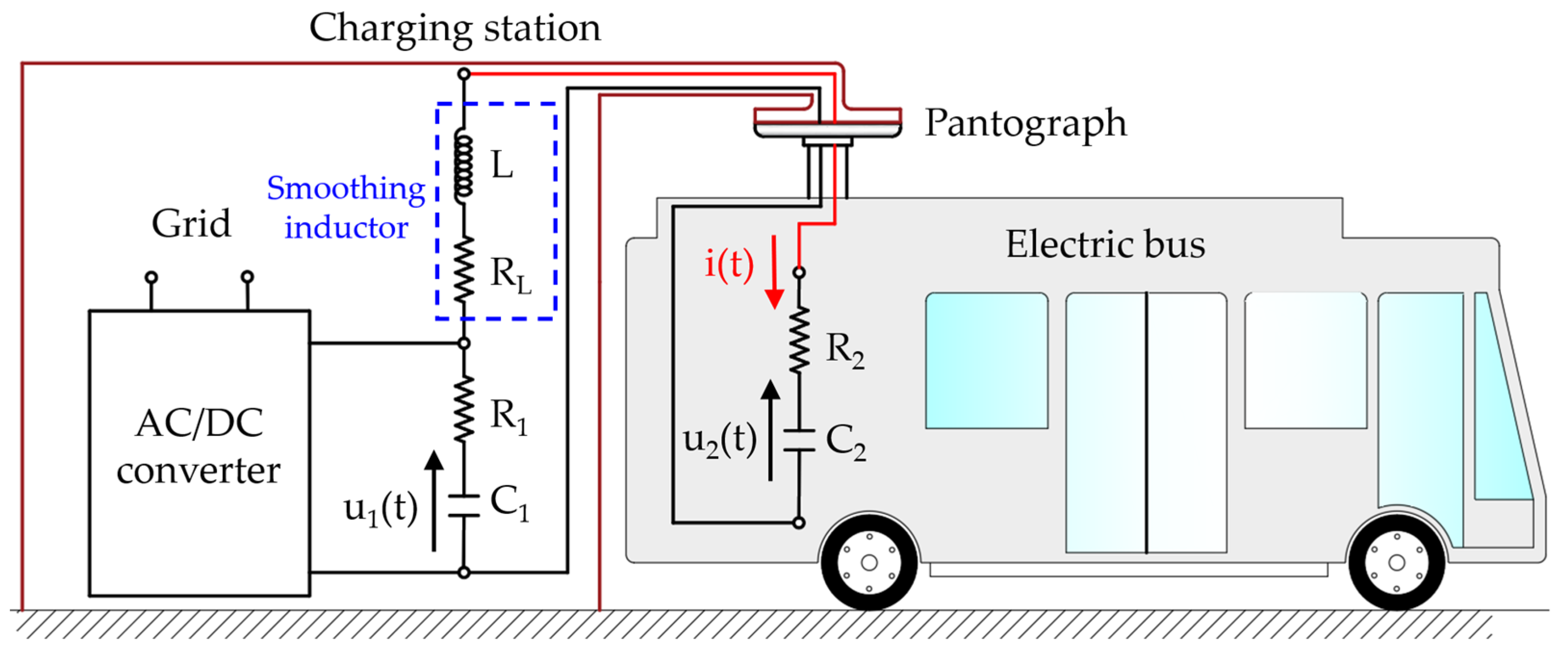
J. F. Pedrayes et al. [32] detail the complete procedure for sizing the charger capacitor bank (npc, nsc, Rcell, Ccell, and U01) and smoothing inductor (RL and L). To do this, it is necessary to know the maximum time allowed to charge the vehicle, tcharge; the maximum peak current allowed during charging, Imax; and the values of the capacitor bank of the electric vehicle (npv, nsv, Cv, and Rv). The calculation of the latter will depend on the demanded power profile by the vehicle and the range to be given, for which the dimensioning method proposed in [43] can be used. In the design of the charger and the smoothing inductor, the aging of the cells (both the charger and the electric vehicle) has been considered, as it will produce changes in the capacitance and internal resistance of both. Figure 1 shows a complete schematic of the fast-charging station (charger-smoothing inductor-electric vehicle), with all branches in parallel. Figure 2 shows a simplified schematic of the set. The AC/DC converter is responsible for raising the voltage of the charger cells to the U01 voltage, once it has discharged part of its energy into the cells of the electric vehicle.
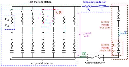
Figure 1.
Wiring diagram of the fast-charging station.
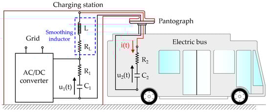
Figure 2.
Simplified diagram of the assembly, once the fast charger is connected to the electric vehicle’s SC bank.
The equivalent resistance and capacitance of the charger (R1 and C1 respective) have the following values:
Once the fast charger is built, the number of serial elements of each string, nsc, will be fixed. However, the number npc of parallel branches that the charger has will vary depending on the initial voltage of the vehicle’s SC bank at the time of connection of both blocks, u2 (t = 0) = U02. Therefore, the R1 and C1 values will be variable. However, in the SC bank of the electric vehicle, both the number of elements in series, nsv, and branches in parallel, npv, will be constant, so that their equivalent resistance and capacitance, R2 and C2, are as follows:
For the thermal analysis, R2 and C2 will be considered constant and with the corresponding values at the beginning of their useful life (0% degree of aging) since this will be the most unfavorable case for the charger from the thermal point of view. However, in the design of the charger, the possible aging of the cells of the electric vehicle has already been taken into account. It is usually considered that, at the end of the useful life, the cells will have doubled the value of their internal resistance, compared with their initial value, while the capacity will have been reduced by 20%. These values may vary slightly depending on the manufacturer, but they are the most common, and these will be considered for charger cells. For the smoothing inductor, no variation in its parameters due to aging has been applied. Knowing that it has a known internal resistance of RL value, the total resistance of the circuit, RT, is as follows:
The equivalent capacitance of the set, Ceq, has the following value:
The total circuit has two energy storage elements: the equivalent capacitance, Ceq, and the smoothing inductor, L. When they are connected by means of the pantograph, a current i(t) will appear (Figure 1), whose time evolution responds to the following second-order ordinary differential equation (ODE):
As indicated in [32], the elements of the fast charger must be sized so that, during the transient state, the assembly behaves as an overdamped system, in order to avoid dangerous voltages, which could damage any of the cells of the assembly, and to minimize the charging time of the electric vehicle.
If the initial voltage of the charger, u1 (t = 0) = U01, and the initial voltage of the vehicle’s SC bank, u2 (t = 0) = U02, are known (U01 > U02), and defining the difference between both as ΔU = U01 − U02, the solution of the ODE given in (7) is as follows:
In expression (8), sinh () is the hyperbolic sine function. The α constant is the damping coefficient of the circuit, which is measured in (s−1). Its value is given by the following:
The resonant pulsation of the circuit is ω0 (s−1), which depends only on the inductor and equivalent capacitance of the circuit, according to the following expression:
The coefficient β that appears in i(t) is defined as damped pulsation and has the same units as α and ω0. Its value is as follows:
From the total current i(t), it is easy to deduce the value of the instantaneous current going through each branch of the charger, isc(t), and each branch of the vehicle’s SC bank, isv(t), as shown in Figure 1, which are as follows:
The time it takes for the energy to be transferred from the charger to the electric vehicle, which will be denoted as tdch, will be equal to the time it takes for both currents to be extinguished. Considering that exponential functions fall to zero after a time whose value is approximately equal to seven times the time constant of the circuit, this time can be calculated with the following expression:
After the tdch time, the circuit will have reached the steady state. All charger values designed in [32] have been chosen so that tdch ≤ tcharge = 30 s, regardless of the initial value of the vehicle’s initial voltage U02 or the degree of aging of any of the cells in the assembly. Other values can be chosen in the design of the fast charger, depending on the needs of the application.
The instantaneous voltages of the equivalent capacitance of the charger, C1, and of the electric vehicle, C2, u1(t) and u2(t), respectively, are obtained directly from the current given in (8) and using the relationship between it and these capacitances. The values of both voltages (Figure 2) are given by the following functions:
If the circuit is allowed to reach the steady state, the two capacitances will converge to the same voltage, the final value of which, Ufinal, will be the following:
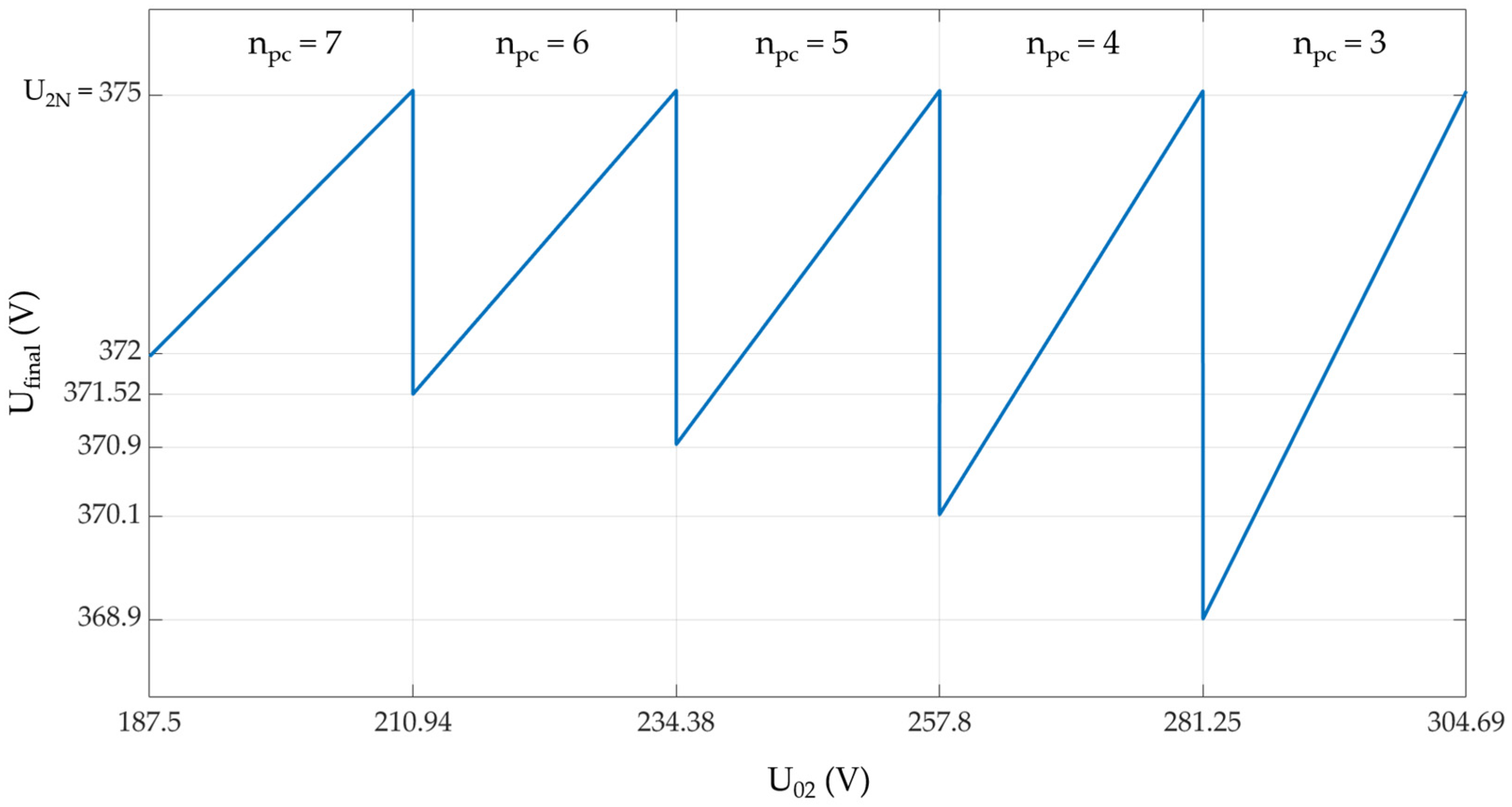
As can be deduced from expression (17), the equivalent capacitance of the charger, C1, must be variable, so that it adapts its value according to the voltage with which the vehicle arrives at the station, U02, so that the final voltage of the assembly, Ufinal, is a value as close as possible to U2N. That is the reason the charger designed in [32] has seven branches connected in parallel, four of which can be disconnected by means of switches. Figure 3 shows what the Ufinal value will be based on the initial voltage of the vehicle, U02, and depending on the number of branches connected to the charger, npc.
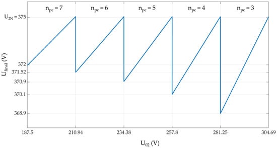
Figure 3.
Ufinal as a function of U02, for different values of npc, which vary between 3 and 7, with the charger and electric vehicle cells being at the beginning of their useful life (0% aging).
2.2. Thermal Analysis of an SC, Working in a Fast-Charging System
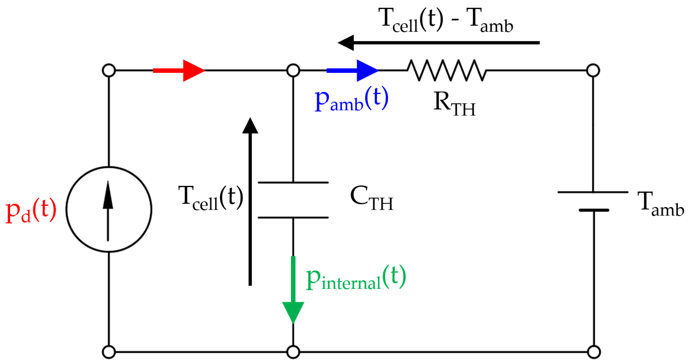
The most used heat transfer model is the equivalent circuit model, which is based on the analogy between a thermal circuit and an electrical circuit (Figure 4). In this model, the dissipated power in the internal resistance of the SC, which is transformed into heat, pd(t), is represented as a current source. The ambient temperature, Tamb, which will be considered constant, is modeled as a voltage source. The passive elements of the model are the thermal resistance, RTH [°C/W], and the thermal capacitance, CTH [J/°C], which appear in the datasheets provided by the manufacturers. In this model, pamb(t) represents the heat dissipated to the environment and pinternal(t) represents the power that increases the internal energy of the cell, i.e., the power that causes an increase in temperature.

Figure 4.
Thermal model of an SC based on an analogy with an electrical circuit [32].
The differential equation that determines the thermal behavior of the cell is as follows:
In (18), θ(t) represents the thermal jump or temperature difference between the cell envelope and the environment temperature, the latter being considered constant.
If an SC of the charger, with internal resistance Rcell, is permanently charged and discharged with the same constant current, Ich, it will dissipate a constant power, with the next value:
If pd(t) is substituted in (18), the value of the thermal jump as a function of time, θ(t), can be obtained by simple integration, and it will have the following function:
The value θ0 in (21) is the initial thermal jump, and τTH being the cells’ thermal time constant, measured in seconds, and equal to the product of the thermal resistance, RTH, multiplied by the thermal capacity, CTH. If the cell is charged and discharged with the same current, Ich, after a long time (between five and seven times the value of τTH), the exponential function will have practically been extinguished, thus reaching a stabilized thermal jump, so that the final temperature of the cell will converge to the following value:
The value given in (22) appears in the datasheets of the commercial cells provided by manufacturers and is usually indicated for various values of the Ich current.
Since the energy transfer from the charger cells to the electric vehicle cells will take only a few seconds, the ambient temperature will be considered to remain constant in that short interval of time. For each individual cell from one of the npc parallel branches that the charger has, whose thermal parameters (thermal resistance and capacitance) are RTH and CTH, respectively, the following ordinary differential equation of constant coefficients can be established, from which the thermal jump, θ(t), can be obtained during the vehicle charging process:
Substituting the value of the current, isc(t), in (23), for its time expression given in (12), yields the following equation:
The ODE given in (24) can easily be transformed into an exact differential equation if it is multiplied by an integrating factor that depends only on time, whose value is as follows:
In this way, the general solution of the equation can be obtained, and the result of which is as follows:
In θ(t), C is the integration constant, which depends on the value of the initial thermal jump. Assuming that θ (t = 0) = θ0, that constant has the next value:
In order to simplify the final expression of θ(t), the following constants can be defined:
The constant k has units [s−1], the constant k1 has units [°C∙s2], and the constants kθ1 and kθ2 are both measured in [°C]. By means of these values, the thermal jump, θ(t), is expressed in a simplified way by the following time function:
This solution gives the same results as if it were solved (24) by numerical methods, without making any approximation. In general, the values of α and β that appear in the function θ(t) have a high value. In addition, α is slightly higher than β. This means that the terms where the exponents of exponential functions are (2∙(α + β)∙t) and (2∙α∙t) decay to zero very quickly, even with very low time values, in the order of milliseconds. For times greater than 1 s, both exponential functions will have practically disappeared, so the thermal jump, θ(t), can be evaluated by the following approximate function:
2.2.1. Internal Power and Power Dissipated to the Environment
The power that is dissipated to the environment expressed as a function of time is equal to the thermal jump divided by the thermal resistance of the cell, as follows:
The power used to raise the internal energy of the cell, i.e., to increase its temperature, is equal to the thermal capacitance multiplied by the derivative with respect to the time of the thermal jump.
In this application of fast chargers, it habitually happens that Pinternal (t) >> Pamb (t), because the discharge times are very short compared with the value of the thermal time constant of any cell in the set. This implies that almost all the power dissipated in the internal resistance of any cell, pd(t), will be used to raise its temperature and will hardly exchange thermal energy with the environment, so that the process can be considered practically adiabatic.
2.2.2. Maximum Temperature Reached during the Electrical Vehicle Charging Process
When the charger is connected to the electric vehicle, a sudden discharge occurs that results in a very high current peak (several hundred amps), which can cause the temperature of the cells, both the charger and the charge, to rise rapidly. It is important to know the maximum temperature that the SCs will reach, as this should not exceed, in most commercial cells, the value of 60 °C. Exceeding this limit would cause irreversible damage. The maximum temperature will take place at the same instant that the temperature jump is maximum. This instant will be denoted by tθmax. Using the approximate expression given in (33), tθmax can be obtained from the following equality:
Solving Equation (36) yields the value of time, :
In expression (37), log(x) represents the natural logarithm of x. The maximum thermal jump is obtained by substituting the value of the given time in (37) into expression (33), after which the following result is obtained:
The constant δ in (38) is dimensionless and has the following value:
The maximum temperature reached by the cell will be equal to the ambient temperature plus this maximum thermal jump.
This formula can be applied to both charger and electric vehicle cells. If the maximum temperature of a charger cell is being evaluated, the calculation of the constant k1 given in (29) will put the number of parallel branches that the charger has at that time in the npc variable, since the total current passing through a branch of the charger will be equal to the total, i(t), divided by that number. If the temperature of an electric vehicle cell is being analyzed, for the same reason, in the calculation of k1, the npc value will be replaced by the npv value, which is the number of parallel branches of the vehicle’s SC bank. This calculation makes it possible to know if, during the discharge of energy from the charger to the vehicle, knowing the initial temperature of the cell analyzed and the ambient temperature, the cell could suffer an overheating that could be dangerous to its integrity.
2.2.3. Minimum, Average, and Maximum Temperature of Fast Charger Cells in TSS
As soon as the charger releases a part of its stored energy to the cells of the electric vehicle, after which it will have reached a final voltage, Ufinal, it must be recharged to recover the initial voltage, U01, and be ready to perform a new discharge on the next vehicle that arrives at the station. Therefore, the time available to the charger, which will be denoted by tch, to reach that U01 voltage again, starting from the Ufinal voltage, will be less than or equal to the time it takes for the next vehicle to arrive at the charging point. This time will be related to different mobility criteria and depends on many factors, such as the number of vehicles in the line, the average distance between one stop and the next, traffic conditions, the average arrival time that the transport company decides to set for a given stop, the estimated number of passengers to be transported on a route, or even the time of day. Knowing its value will require a complex study that is beyond the scope of this article; however, nowadays, in large cities, it is possible to establish direct communication between each vehicle and its next charging station. Depending on the circumstances at any given time, it is possible to estimate, in real time, how long it would take for a vehicle to reach its next stop. Since these times depend on many factors, this study will consider several values with which to draw conclusions.
Normally, the recharging of the fast charger will be carried out at a constant current, Ich. If the time available for recharging is high, it can be done with a low current, which will improve performance. This will also make the average temperature of the charger’s SCs lower, which will extend its useful life. Therefore, in this application, it will be considered that the charger takes advantage of the maximum time it has, tch, to charge with the minimum possible current, since it is the best option, both from the thermal point of view and from the efficiency of the charging process. The value of the current Ich needed to increase the voltage from Ufinal to U01 at time tch is as follows:
In (41), it should be noted that the C1 value will depend on how many branches in parallel need to be recharged, since it is possible that not all of them would have been connected in the previous discharge to the electric vehicle, if the latter had arrived with a high initial voltage. The lower the Ufinal voltage and the shorter the available charging time, tch, the higher the Ich current.
If the fast charger must supply energy to a fleet of vehicles that are constantly on the road, working 12 or more hours a day [44], its cells will be cyclically subjected to constant charging currents and high discharge currents on the vehicles. If this is maintained over time, the TSS will be reached, in which the temperature of the charger cells will stabilize and oscillate around an average value, reaching a maximum at the end of the heating stage (during discharge to the electric vehicle) and a minimum at the end of charging from the grid at a constant current. The maximum, minimum, and average temperature values will depend on the time available to recharge from the main supply source, tch, and the ambient temperature, among other factors.
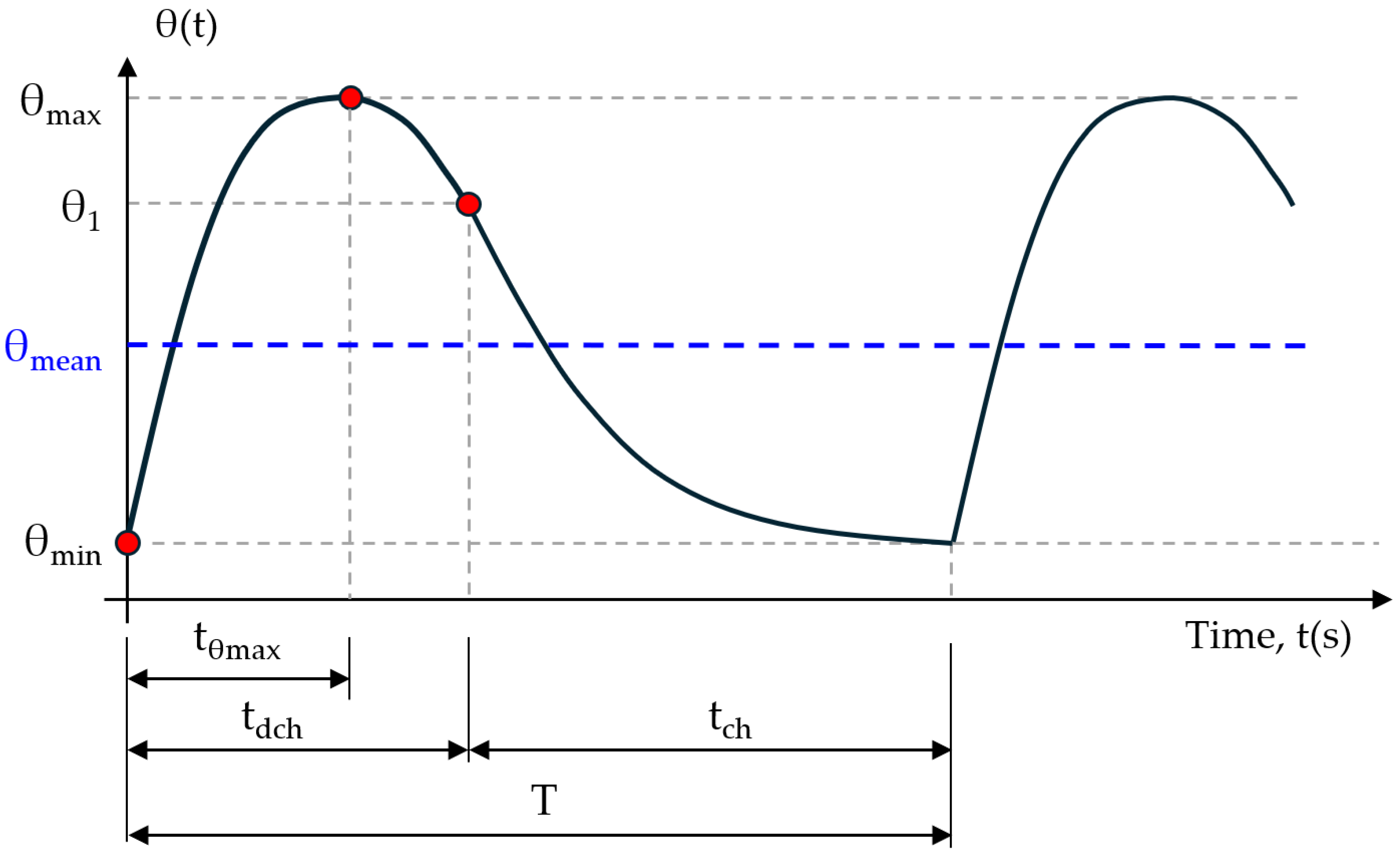
If the charger cells are in TSS with a minimum thermal jump θmin, and at that moment they transfer back their energy on the vehicle cells, when the discharge time, tdch, has elapsed, they will have reached a thermal jump θ1, which, in general, will not be equal to the maximum value (this last one shall take place at the instant < tdch) (Figure 5). Next, if the cells of the charger are recharged from the grid with a constant current of value Ich, a current of value Ich/npc will flow through each cell of a string, where npc is the number of parallel branches the charger has at that moment. Considering that, as soon as the charging process from the grid is finished, the energy is transferred back into a vehicle arriving at the station, without intermediate rest intervals, after the charging time, tch, the cells will have cooled down to the initial value, θmin, and the process will be repeated cyclically. Under these circumstances, the current and temperature waves in a cell of the charger will be periodic functions of the period T = tch + tdch. Figure 5 shows the thermal jump evolution once the TSS is reached.
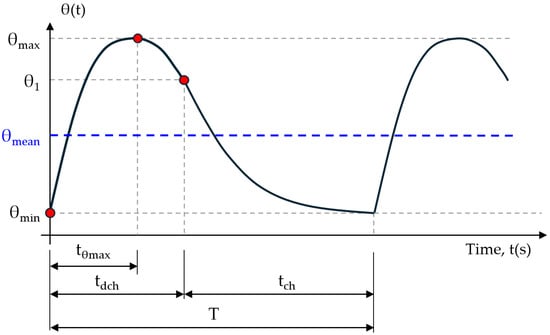
Figure 5.
Thermal jump, θ(t), for one of the cells of the fast charger once steady state is reached.
In order to obtain the value θmin, it is necessary to solve the following system of equations:
The value θ1 is not important, although this additional equation is necessary to determinate θmin, which in turn will be needed to calculate the maximum thermal jump, θmax, and the mean thermal jump, θmean, which are the ones that are important to know. In this case, the approximate function for the calculation of θ(t) has been used (33), in the vehicle discharging phase, since, at the instant tdch, the difference between the value provided by this function and the one obtained with the exact formula (32) is practically zero. Solving the system given in (42) gives the following result for θ1 and θmin:
In both θ1 and θmin, the term of the exponential function whose exponent is negative and of a very high absolute value has been neglected since it is practically zero. To obtain the maximum thermal jump, θmax, it must be taken into account that the function θ(t) during the heating phase can be expressed as follows:
The maximum value can be calculated from Formulae (38) and (39) by simply replacing the initial thermal jump, θ0, by the minimum thermal jump, θmin, given in (44). The mean thermal jump, θmean, that the cell will reach can be obtained by considering the function of power dissipated in the cell as a function of time. This function can be defined in sections as follows:
The mean dissipated power will then be given by the following integral:
Solving (47) and taking into account that, for the instant tdch, the value of the function exp(−2∙α∙tdch) can be considered practically zero, it is finally concluded that the mean value of the power dissipated is as follows:
The mean thermal jump will be equal to the product of the mean dissipated power and the thermal resistance. Substituting the values of α and β according to expressions (9) and (11), it finally follows that
The mean temperature of the analyzed cell will then be as follows:
3. Results and Discussion
In this section, several simulations will be carried out to assess how the temperature of the cells of the charger and the electric vehicle would evolve under different circumstances, and the results obtained will be compared with the formulae developed in Section 2 in order to check their validity. For this purpose, the data of the fast charger sized in [32] will be used, which has been designed for the discharge of part of its energy on an electric minibus of the brand Tecnobus Gulliver U500TM, which is a hybrid vehicle consisting of a 120 Ah (72 V) lead-acid battery and a bank of SCs of the manufacturer Maxwell TechnologiesTM of 375 V nominal voltage and 21 F capacity. The minibus has a pantograph from the manufacturer SchunkTM to connect to the fast charging station. All its features can be found in [30], where the testing of a fast charging prototype, also based on SCs, but with a slightly different topology from the one proposed in [32], is analyzed.
3.1. Single Discharge with No Repetition
In this first example, it will be considered that the initial voltage of the vehicle’s SC bank is U02 = 187.5 V; therefore, the charger will have all the branches connected in parallel (npc = 7), which will provide the maximum capacitance of the charger. It will be assumed that both the charger and the electrical bus cells are at the beginning of their useful life, so that their degree of aging is nil. From the cells data of the charger and the electric vehicle, shown in Table 1 and Table 2, the values corresponding to the internal resistance and equivalent capacitance of the charger (R1, C1) and the electric vehicle (R2, C2) are obtained. These data are shown in Table 3, as well as the values corresponding to the smoothing inductance (L, RL), the initial voltage of the charger (U01), and the electric vehicle (U02).
Table 3.
Equivalent circuit data.
From the data shown in Table 3, the parameters RT, Ceq, α, ω0, and β, calculated from expressions (5), (6), (9), (10), and (11), respectively, are derived, which are necessary to calculate the total circuit current, i(t), and the temperature of the cells. These values are shown in Table 4. There also appears the value of the time that it is needed to charge to the electric vehicle, tdch, given by (14).
Table 4.
Equivalent circuit data (RT, Ceq, α, ω0, β, tdch, and ∆U).
For the charger design, cells of the same type as those of the electric vehicle have been selected. These cells are manufactured by Maxwell TechnologiesTM and possess a nominal capacitance of 3000 F and an internal resistance of 0.15 mΩ. Therefore, the thermal parameters of these cells are identical for the fast charger cells as for the electric vehicle SC bank. These parameters are summarized in Table 5, which also includes the ambient temperature, Tamb, utilized in this example, as well as the constants k, k1, kθ1, and kθ2 as defined in (28), (29), (30), and (31), respectively.
Table 5.
Thermal data (RTH, CTH, τTH, k, k1, kθ1, kθ2, and Tamb).
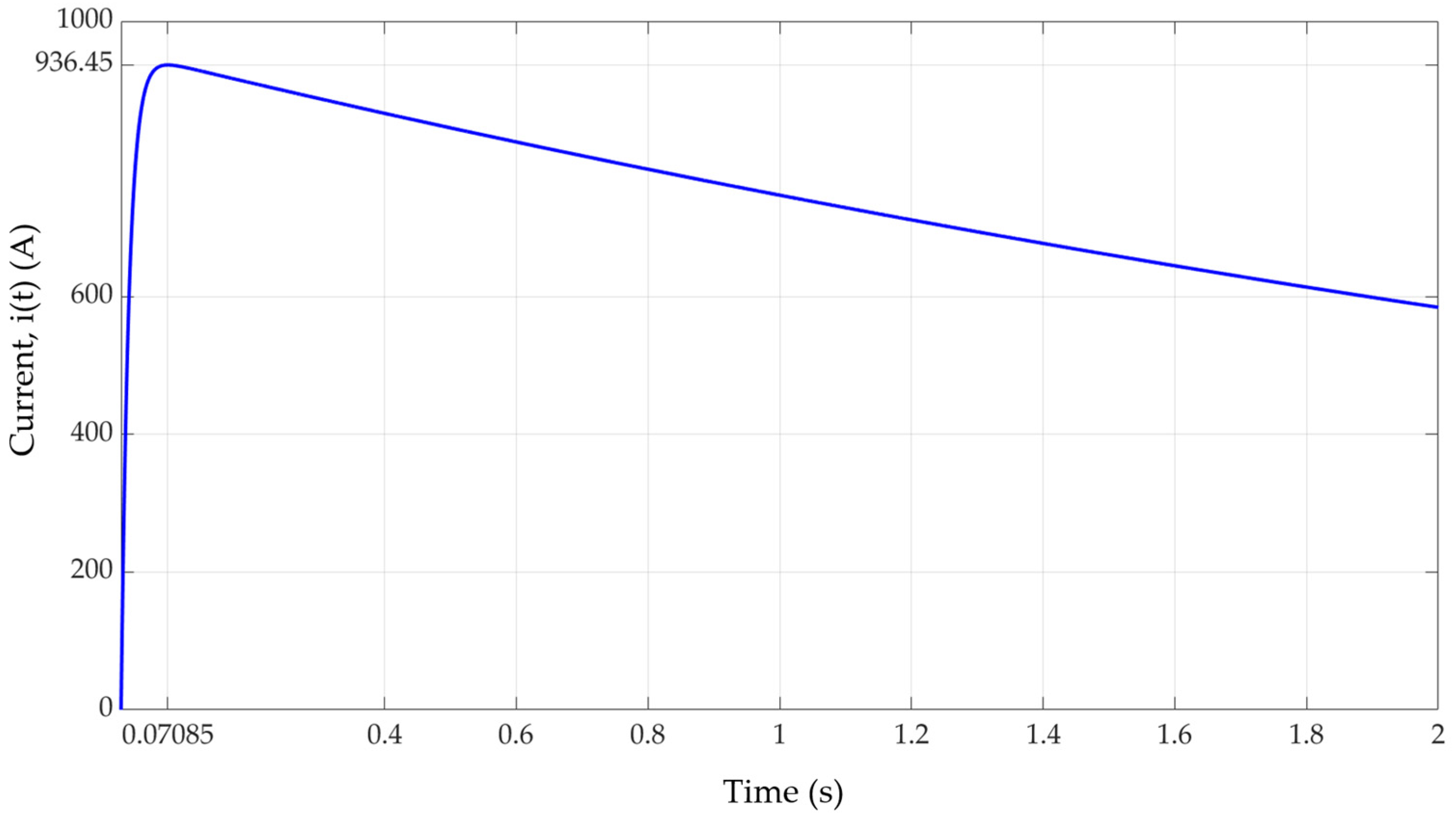
Referring to the information presented in Table 5, when examining a single cell from the electric vehicle, and considering that, in this scenario, npv = 1, the current passing through it equals the total current, denoted as i(t). The time function of this current, derived from the expression provided in (8), is described as follows:
Figure 6 shows how the current i(t) evolves in the first 2 s, which reaches a maximum value of 936.45 A at the instant t = 70.85 ms.

Figure 6.
Circuit current, i(t), as a function of time, for the first 2 s.
Taking into consideration that the cell begins at ambient temperature (θ0 = 0 °C) and referencing the data provided in Table 5, the thermal jump can be computed over time, using the expression specified in (32):
The approximate thermal jump follows a similar function, achieved by eliminating the terms where the exponents of the exponential functions are larger. Its function would look like this:
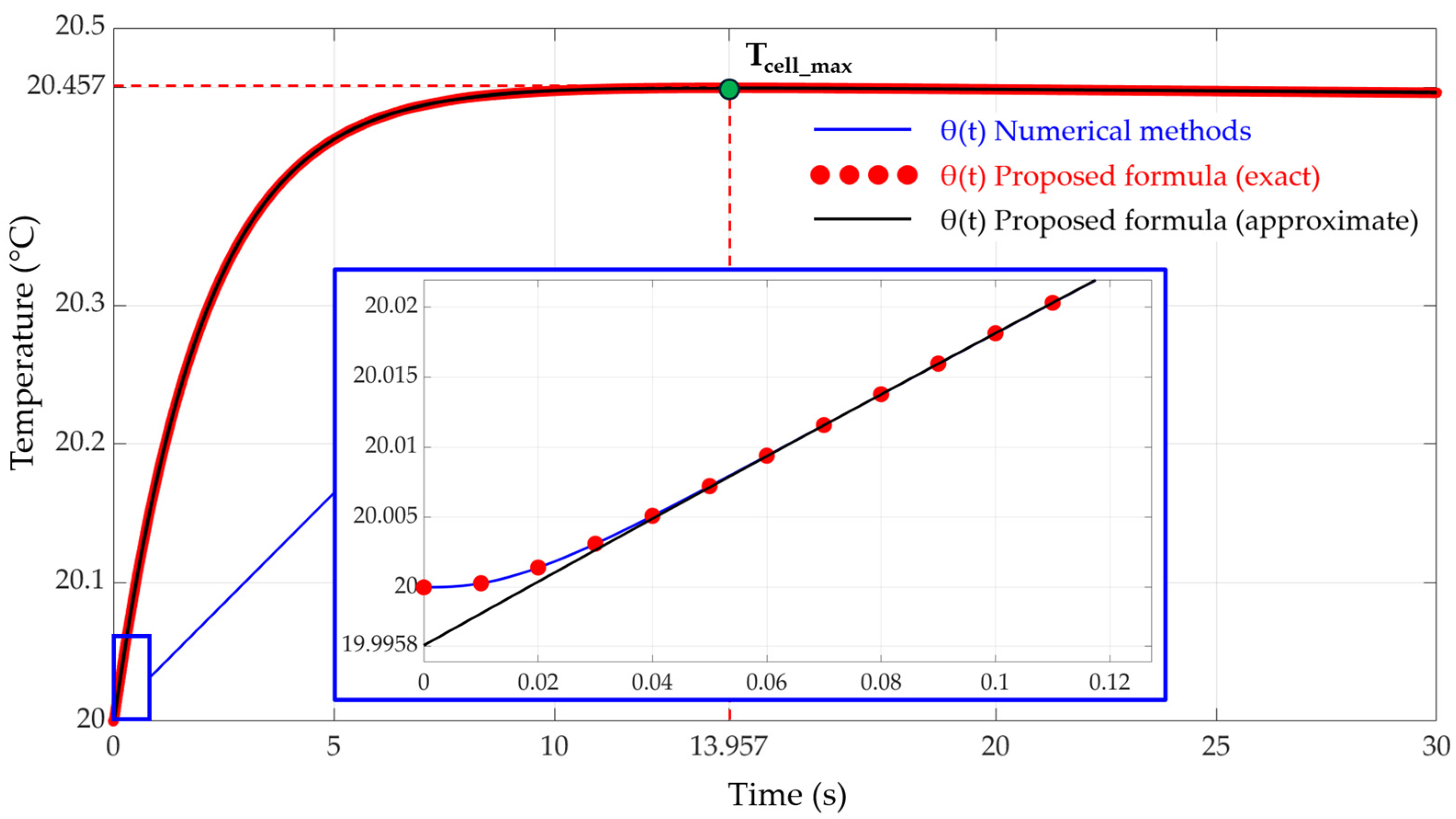
The cell temperature is determined by adding the ambient temperature to the thermal jump. Figure 7 illustrates the temperature profile of an electric vehicle cell, considering θ(t) using the exact Formula (52) (represented by red dots), the approximate Formula (53) (depicted by a black line), and the solution obtained by numerically solving the differential Equation (24) (illustrated by a blue line).
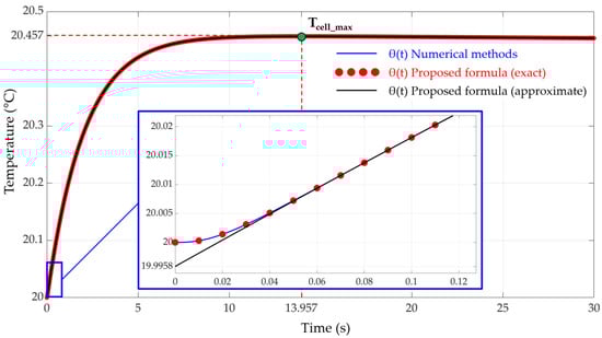
Figure 7.
Temperature evolution over time of one of the cells of the electric vehicle, using numerical methods (blue line), the exact proposed formulation (32) (red dots), and the approximate formula (33) (black line).
The approximate function deviates only slightly from the exact function in the initial milliseconds. However, from 50 ms onwards, all three functions converge and become identical. The instant at which the maximum temperature value occurs can be calculated from expression (37), which, in this example, gives the value . The temperature evaluated at that instant, using the exact (32) or approximate (33) formula, gives 20.457 °C, as can be seen in Figure 7.
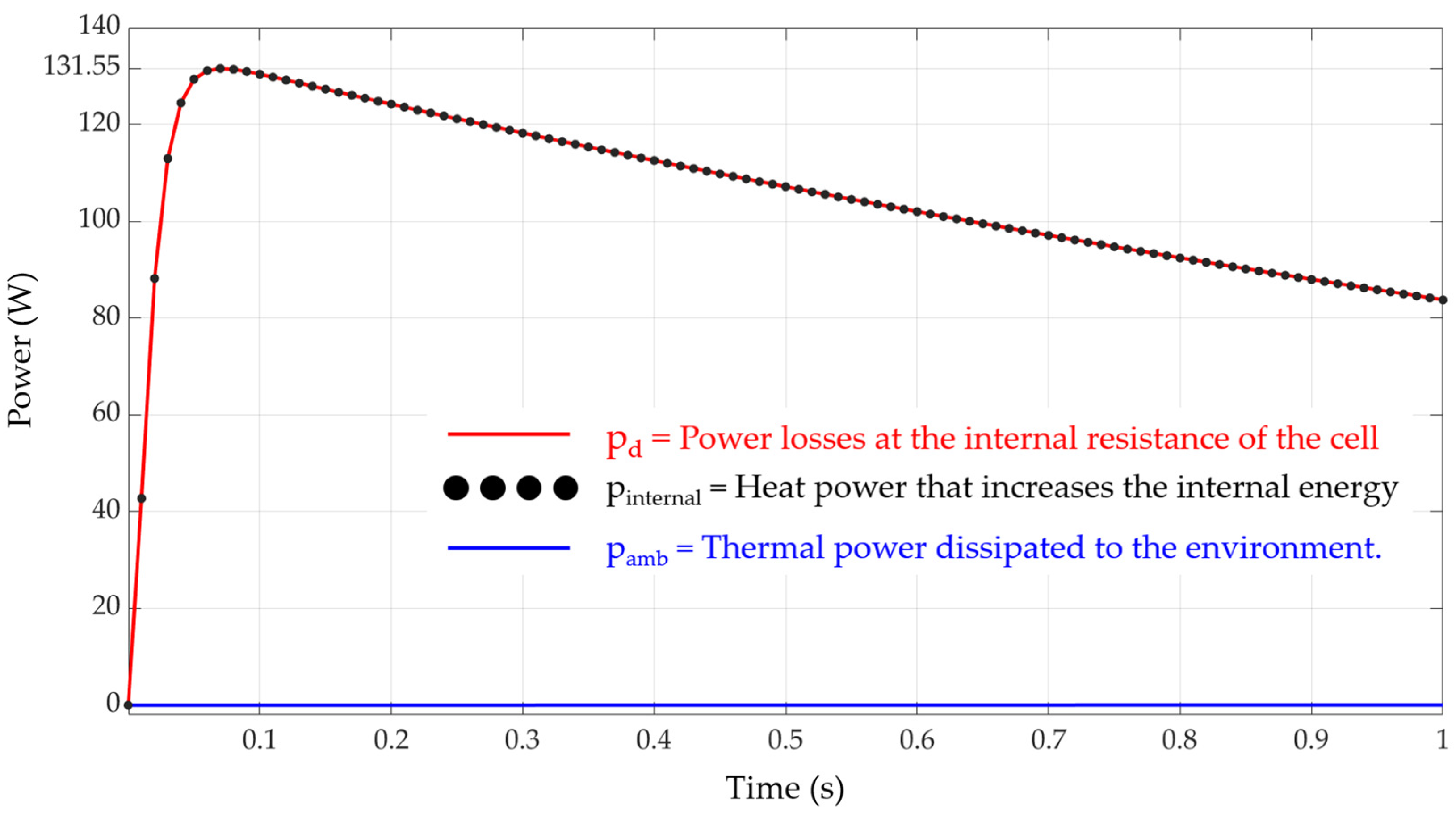
Figure 8 shows the power dissipated to the environment, pamb(t), given by (34) (blue line); the internal power, pinternal(t), responsible for the temperature rise (black dots), calculated with expression (35); and the power dissipated within the internal resistance of the cell, pd(t) (red line), which is the sum of the two previous ones, as shown in the thermal model of Figure 4. As can be seen, the power dissipated in the cell is almost equal to the internal power, so the heating process can be considered practically adiabatic.

Figure 8.
Power generated in the internal resistance of the cell, pd(t) (red line); heat power that increases the internal temperature of the cell, pinternal(t) (black dots); and power dissipated to the environment, pamb(t) (blue line).
3.2. Continuous Charging and Discharging of the Charger until the TSS Is Reached
In this second example, the simulation will show the temperature evolution of the charger cells when subjected from the grid to constant current charging Ich, over a time tch, succeeded by discharging onto the electric vehicle. This process will be repeated until reaching the TSS. The electric vehicle will again be assumed to arrive at the charging station with the initial voltage U02 = 187.5 V. In the charger, all seven branches will be connected (considering all cells at the beginning of their lifetime); therefore, it will have an equivalent capacitance C1 = 138,158 F, and the final voltage at which the set (charger and electric vehicle) will reach will be equal to Ufinal = 372 V (Figure 3).
If it is considered that the time for the charger to go from Ufinal to U01 = 400 V is tch = 300 s, the charging current required for this, according to expression (41), will be Ich = 12.895 A. This current can be considered sufficiently low so as not to cause any harmful effect on the grid to which the converter supplying it will be connected. Since the discharge time on the vehicle, under these circumstances, is tdch = 28.45 s (Table 4), the cell temperature will be a periodic function of period T = 328.45 s. The TSS would be reached after approximately the 5∙τth value = 9600 s (2 h 40 min).
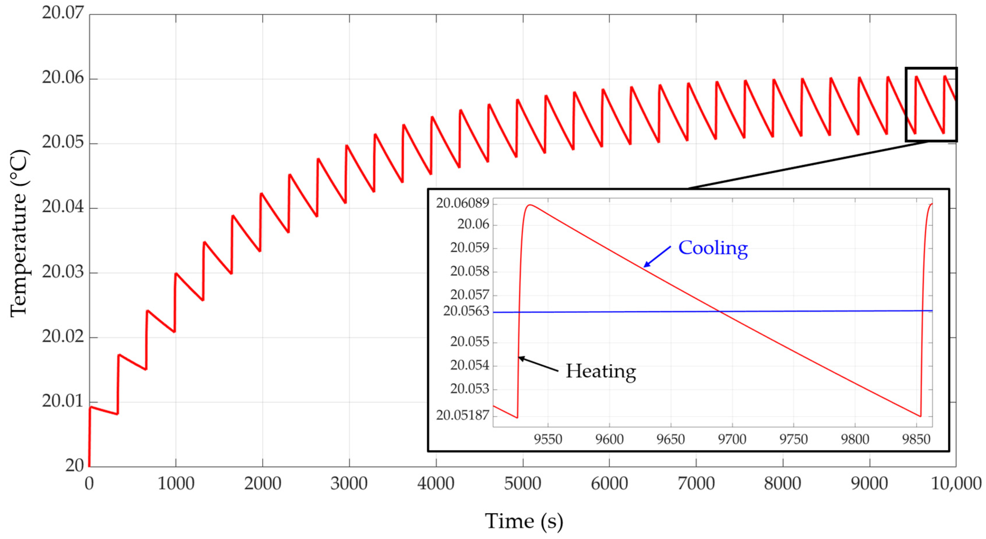
Figure 9 shows the evolution of the temperature of the charger cells over time, working continuously under these circumstances. In this case, the graph has been obtained using numerical methods. It can be seen that, once the TSS has been reached, the mean temperature will be Tmean = 20.0563 °C, which can be calculated by means of expression (50). The minimum and maximum temperatures, which are obtained by adding to the ambient temperature the minimum and maximum thermal jumps, given in (44) and (38), respectively, are Tmin = 20.05187 °C and Tmax = 20.06089 °C, as can be seen in the same figure. During the phase of energy transfer to the vehicle (heating), the temperature of the cells will transition from Tmin to Tmax. Conversely, during the constant current charging phase from the grid, the cells will transition from Tmax to Tmin (cooling), thus completing the entire cycle. Based on these findings, it is evident that, despite the passage of current through the cells, with a maximum value reaching 133.78 A (Imax/7), their temperature increase relative to the ambient environment is minimal. Therefore, with proper control, there is no risk of the charger cells sustaining damage due to overheating.
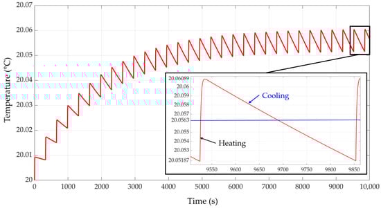
Figure 9.
Temperature evolution of the charger cells, considering a time tch = 300 s with a current Ich = 12.895 A, until the TSS is reached.
The above example is not the most unfavorable case for charger cells from a thermal point of view. If both these and those of the electric vehicle are at the beginning of their lifetime (0% aging) and all seven charger branches are connected, the peak value of the total current i(t), Imax, will be the highest possible (936.45 A). Figure 6 shows the time evolution of i(t), in which this maximum can be verified. Figure 10 shows the Imax value for different degrees of aging of the fast charger cells and the electric vehicle cells depending on the number of modules connected to the fast charger during discharge to the electric vehicle.
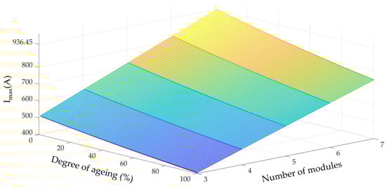
Figure 10.
Peak value of total current i(t), Imax (A), for a different number of modules and different degrees of aging of the cells.
If the charger, instead of seven connected branches, had six, which would be the case if the electric vehicle had arrived at the station with an initial voltage U02 between 210.94 V and 234.38 V (Figure 3), the ∆U value would be lower and the total resistance, RT, would be higher. These two factors would reduce the total current, but it should be noted that, according to the expression for isc(t) given in (12), this would be equal to i(t) divided by six, rather than by seven. This would make the current of each branch of the charger, isc(t), higher. Of the three factors, the last one has the most influence, so if the number of parallel branches of the charger is reduced, although the total current i(t) decreases, the current of each branch, isc(t), will increase.
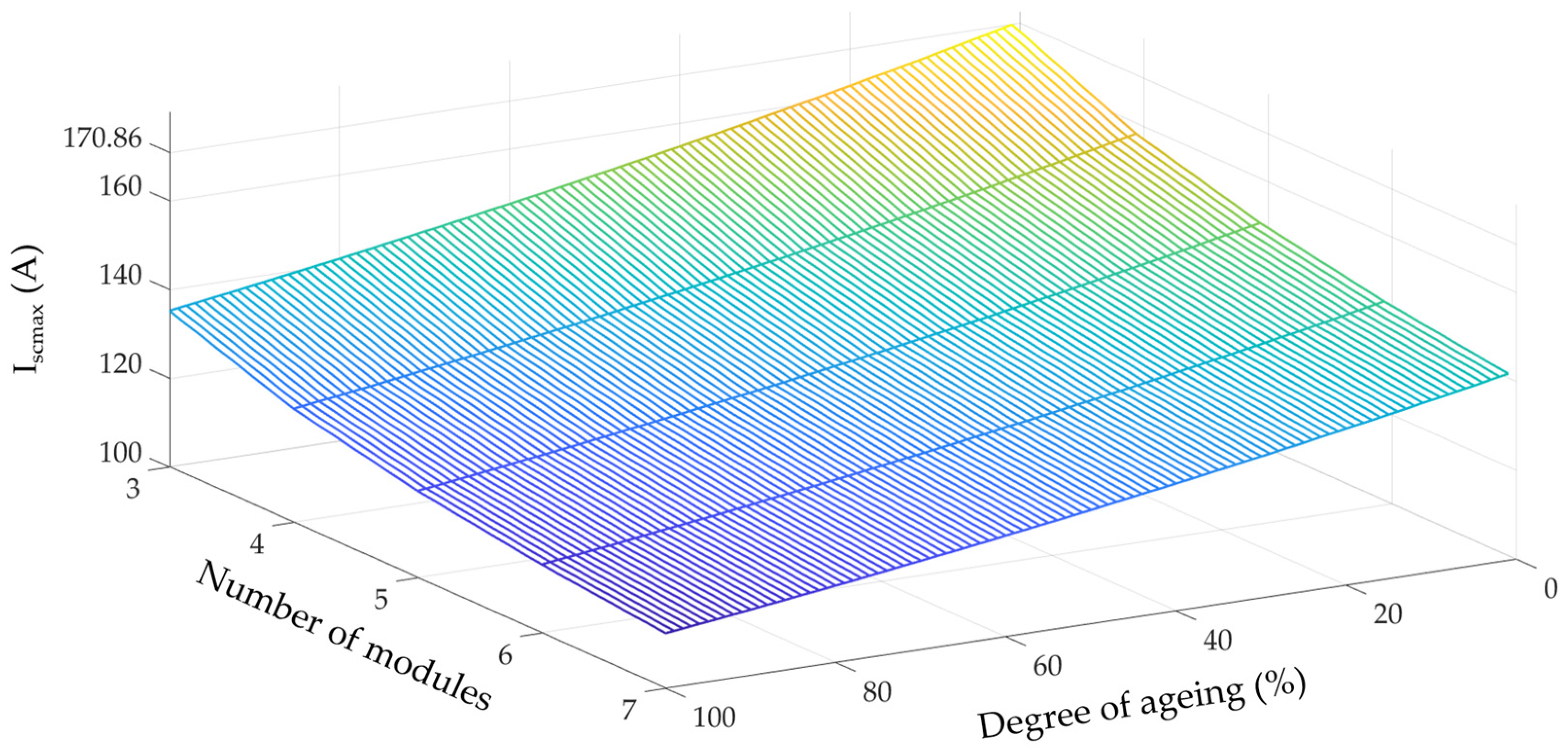
Figure 11 shows the peak current value of any of the charger branches, Iscmax, as a function of the number of branches connected and the degree of aging of the cells, both in the charger and in the electrical vehicle. The highest value of Iscmax would be given with the minimum possible number of parallel branches of the charger (nsc = 3) and with all the cells of the whole set at the beginning of their lifetime, reaching 170.86 A in this example.
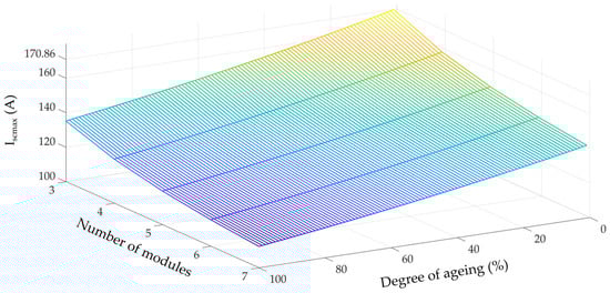
Figure 11.
Maximum current that would appear on each branch of the charger, Iscmax (A), for a different number of modules and different degrees of aging of the cells.
However, this is not the worst possible scenario either. If the charger cells were at the end of their useful life (100% aging), their resistance would be double the resistance they had at the beginning of their useful life, but this would have little effect on the total resistance, RT, since the resistance of the electric vehicle, R2 (which has fewer branches in parallel than the charger, in this particular case), and the smoothing inductance, RL, have the greatest influence. This means that RT would be only slightly higher than if all cells were new, so the current in each branch, isc(t), would be almost the same with new or aged charger cells, while the power dissipated in each charger cell, which is Rcell ∙ isc(t)2, would be much higher as the value of Rcell doubles due to aging. Figure 12 shows the maximum power dissipated in a charger cell, Pdmax (W), considering the charger cells aged at 100% and the electric vehicle cells aged at 0%. The maximum value reached in this case would be 8.17 kW.
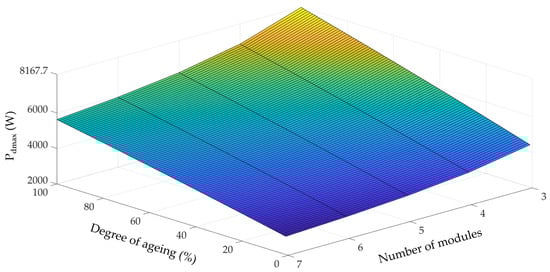
Figure 12.
Maximum power dissipation, Pdmax (W), in each charger cell, for a different number of modules and different degrees of aging of the cells.
From the point of view of the heating of the charger cells, the worst possible scenario would be one in which the electric vehicle arrives with the lowest possible voltage within the interval in which the charger is obliged to connect the minimum number of branches (nsc = 3), which in the example given in [32] would be U02 = 281.25 V (∆U = 118.75 V) and, in addition, in which the cells of the electric vehicle have an aging level of 0% and those of the charger are at 100% (practically at the end of their useful life). In this case, the capacitance of the charger would be C1 = 47.368 F, which means that the final voltage at which the assembly will arrive, according to (17), will be Ufinal = 363.524 V. Although this situation is highly unlikely, it would lead to the maximum power dissipation in the charger cells and, consequently, the highest attainable temperature.
Based on this hypothetical situation, which is the most unfavorable, the following shows the minimum, mean, and maximum thermal jump of the charger cells, operating in continuous mode and having reached the TSS, as a function of the charging time, tch. The values needed to simulate this case are shown in Table 6 and Table 7. No variation of the thermal parameters (RTH and CTH) due to cell aging has been considered.
Table 6.
Charger data (with 100% aging) and equivalent circuit data.
Table 7.
Thermal data (RTH, CTH, τTH, k, k1, kθ1, and δ).
The functions θmin(tch), θmean(tch), and θmax(tch) are obtained from the formulae shown in (44), (49), and (38), respectively. Their values are as follows:
Figure 13 shows the θmin(tch), θmean(tch), and θmax(tch) functions for values of tch between 200 and 600 s. The values of the three functions are shown for charging times, tch = 200 s, tch = 300 s, and tch = 500 s.
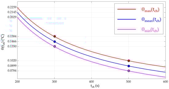
Figure 13.
Functions θmin(tch) (lower), θmean(tch) (middle), and θmax(tch) (upper), corresponding to expressions (54), (55), and (56), respectively, for values of tch between 200 and 600 s.
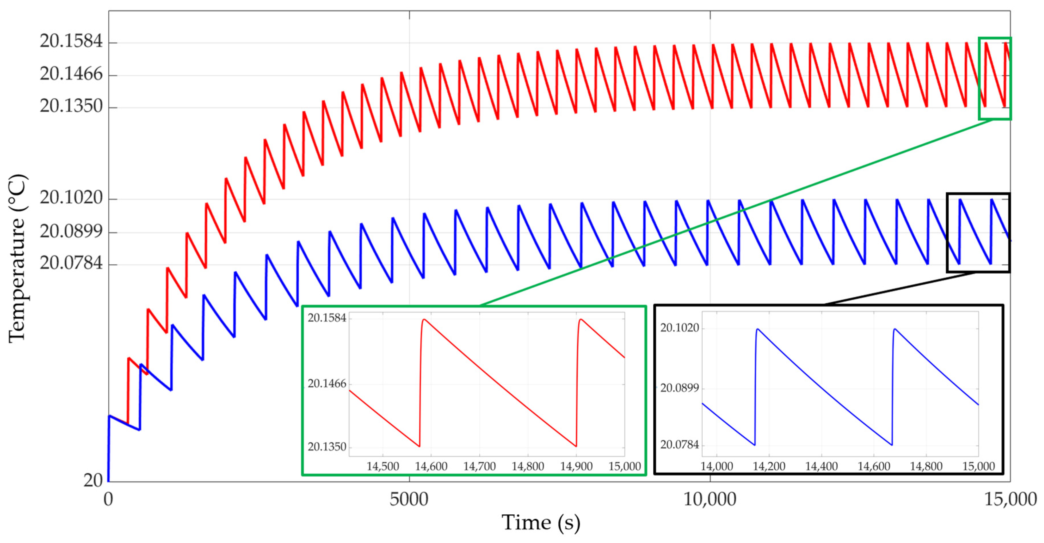
Figure 14 illustrates the temperature profile of one of the charger cells for two different recharge time values, tch = 300 s and tch = 500 s, obtained by simulation and considering Tamb = 20 °C. The θmin, θmean, and θmax values achieved can be seen in Figure 13. The higher the tch value, the lower the three values.
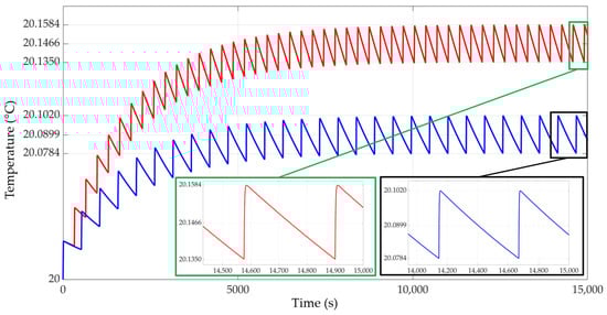
Figure 14.
Temperature of a 100% aged cell of the fast charger, working in steady state, with npc = 3 and considering Tamb = 20 °C, for charging times tch = 300 s (red line) and tch = 500 s (blue line), with U02 = 281.25 V.
4. Conclusions
In this contribution, the analytical expressions necessary for the calculation of the instantaneous temperature of the SCs of a fast charger during the energy discharge process on the electric vehicle have been obtained. The formulae are equally valid for the SCs mounted on the latter. The analysis includes the calculation of the maximum temperature value and the instant at which it occurs, as well as the average, minimum, and maximum temperature values for the charger cells once the thermal steady state is reached, considering charging at a constant current and with different recharge times. The results of the formulae have been compared with those obtained using numerical methods in order to check their validity. These formulae can be used for any charger using the topology described in [32].
Based on the theoretical analysis, the thermal behavior of the charger has been studied under different circumstances—different charging times, different degrees of cell aging, etc. The maximum temperature that the cells of the electric vehicle would reach during the charging process has also been calculated.
Based on the analysis of the example and the results obtained from simulations, it is evident that, with this charger topology, none of its cells will ever reach dangerous temperature levels that could cause damage, even under scenarios involving very short recharge times or extremely high current peaks during discharge to the electric vehicle. It has also been verified that, when the charger is operating in continuous mode and once the TSS has been reached, even in the most unfavorable situation, the mean temperature of the cells will hardly be increased by its operation in the fast charger, and it will be only slightly higher than the ambient temperature. This means that cell aging will be determined mainly by environmental conditions. Finally, it can also be deduced that this system would not need any forced cooling system, since its thermal jump with respect to the environment would be very low, so that, under normal conditions, the cells will remain below 60 °C.
Author Contributions
Conceptualization, J.F.P.; methodology, J.F.P. and M.F.Q.; software, M.F.Q., M.F.C. and E.E.V.Z.; validation, M.F.Q., G.A.O. and M.F.C.; formal analysis, J.F.P. and M.F.C.; investigation, M.F.Q., J.F.P. and G.A.O.; writing—original draft preparation, J.F.P.; writing—review and editing, E.E.V.Z., G.A.O., M.G.M. and M.F.C.; supervision, E.E.V.Z. and M.G.M.; project administration, M.G.M. and M.F.Q.; funding acquisition, M.G.M. and G.A.O. All authors have read and agreed to the published version of the manuscript.
Funding
This work was supported by the Spanish Government, MCIN/AEI/FEDER, and the EU, under grants PID2021-122704OB-I00 and TED2021-131498B-I00.
Institutional Review Board Statement
Not applicable.
Informed Consent Statement
Not applicable.
Data Availability Statement
Data are contained within the article.
Conflicts of Interest
The authors declare no conflicts of interest.
Glossary
| R1 | equivalent charger resistance [Ω] |
| C1 | equivalent charger capacitance [F] |
| Ccell | capacitance of each SC of the charger [F] |
| Rcell | resistance of each SC of the charger [Ω] |
| npc | number of charger branches (strings) connected in parallel |
| npcmin | minimum number of charger branches (strings) connected in parallel |
| npcmax | maximum number of charger branches (strings) connected in parallel |
| nsc | number of cells connected in series on each branch of the charger |
| R2 | equivalent resistance of the vehicle accumulator [Ω] |
| C2 | equivalent capacitance of the vehicle accumulator [F] |
| npv | number of branches connected in parallel of the vehicle SC bank |
| nsv | number of cells connected in series on each branch of the vehicle SC bank |
| Rv | resistance of each SC of the vehicle SC bank [Ω] |
| Cv | capacitance of each SC of the vehicle SC bank [F] |
| Ceq | equivalent capacitance of the whole system [F] |
| L | inductance of the smoothing inductor [H] |
| RL | internal resistance of the smoothing inductor [Ω] |
| RT | equivalent resistance of the whole system [Ω] |
| u1(t) | internal instantaneous voltage of the charger [V] |
| U01 = u1(t = 0) | initial internal voltage of the charger [V] |
| u2(t) | internal instantaneous voltage of the vehicle accumulator [V] |
| U02 = u2(t = 0) | initial internal voltage of the vehicle accumulator [V] |
| U02min | minimum initial internal voltage of the vehicle accumulator [V] |
| U02max | maximum initial internal voltage of the vehicle accumulator [V] |
| U2N | rated voltage of the vehicle accumulator [V] |
| ΔU | initial voltage difference between charger and vehicle accumulator = U01 − U02 [V] |
| Ufinal | final voltage of charger and vehicle accumulator (steady state) [V] |
| i(t) | overall instantaneous current [A] |
| α | damping coefficient = 0.5 RT/L [s−1] |
| ω0 | resonance pulsation = (L·Ceq)−0.5 [s−1] |
| β | damped pulsation = (α2 − ω02)0.5 [s−1] |
| τ | electrical time constant of the whole system = (α − β)−1 [s] |
| tch | time available to the charger to raise its voltage from Ufinal to U01 [s] |
| Ich | constant current used to recharge the fast charger [A] |
| tdch | time it takes to discharge from the charger to the electric vehicle [s] |
| T | period of Tcell (t) and i(t) once reached thermal steady state [s] |
| tcharge | maximum charging time [s] |
| tImax | time instant at which the maximum overall instantaneous current occurs [s] |
| Imax | maximum circuit current [A] |
| isc(t) | current passing through one of the charger’s branches [A] |
| isv(t) | current passing through one of the branches of the electric vehicle’s SC bank [A] |
| Iscmax | maximum current reached in one of the charger branches [A] |
| pamb(t) | thermal power dissipated to the environment [W] |
| pd(t) | instantaneous dissipated power [W] |
| Pdmean | mean power dissipated once the thermal steady state has been reached [W] |
| Pdmax | maximum power dissipated in one of the charger cells [W] |
| pinternal(t) | heat power that increases the thermal energy stored in the SC [W] |
| Tcell (t) | instantaneous cell temperature [°C] |
| T0 | initial cell temperature [°C] |
| Tmax | maximum cell temperature [°C] |
| Tmean | mean cell temperature once the thermal steady state has been reached [°C] |
| Tamb | ambient temperature [°C] |
| θ(t) | thermal jump [°C] = Tcell − Tamb |
| θ0 | initial thermal jump [°C] = T0 − Tamb |
| θmin | minimum thermal jump once the thermal steady state has been reached [°C] |
| θmean | mean thermal jump once the thermal steady state has been reached [°C] |
| θmax | maximum thermal jump once the thermal steady state has been reached [°C] |
| θ1 | thermal jump after the tdch time has elapsed [°C] |
| RTH | thermal resistance of an individual charger cell [°C/W] |
| CTH | thermal capacitance of an individual charger cell [J/°C] |
| τTH | thermal time constant of an individual charger cell [s] |
| k | constant [s−1] |
| k1 | constant [°C∙s2] |
| kθ1 | constant [°C] |
| kθ2 | constant [°C] |
| δ | dimensionless constant |
References
- Yang, Y.; Han, Y.; Jiang, W.; Zhang, Y.; Xu, Y.; Ahmed, A.M. Application of the Supercapacitor for Energy Storage in China: Role and Strategy. Appl. Sci. 2022, 12, 354. [Google Scholar] [CrossRef]
- Muzaffar, A.; Ahamed, M.B.; Deshmukh, K.; Thirumalai, J. A review on recent advances in hybrid supercapacitors: Design, fabrication and applications. Renew. Sustain. Energy Rev. 2019, 101, 123–145. [Google Scholar] [CrossRef]
- Peng, H.; Wang, J.; Shen, W.; Shi, D.; Huang, Y. Compound control for energy management of the hybrid ultracapacitor-battery electric drive systems. Energy 2019, 175, 309–319. [Google Scholar] [CrossRef]
- Joshi, M.C.; Samanta, S. Improved Energy Management Algorithm With Time-Share-Based Ultracapacitor Charging/Discharging for Hybrid Energy Storage System. IEEE Trans. Ind. Electron. 2019, 66, 6032–6043. [Google Scholar] [CrossRef]
- Bolborici, V.; Dawson, F.P.; Lian, K.K. Hybrid Energy Storage Systems: Connecting Batteries in Parallel with Ultracapacitors for Higher Power Density. IEEE Ind. Appl. Mag. 2014, 20, 31–40. [Google Scholar] [CrossRef]
- Zhao, C.; Yin, H.; Ma, C. Equivalent Series Resistance-based Real-time Control of Battery-Ultracapacitor Hybrid Energy Storage Systems. IEEE Trans. Ind. Electron. 2020, 67, 1999–2008. [Google Scholar] [CrossRef]
- Zahedi, R.; Ardehali, M.M. Power management for storage mechanisms including battery, supercapacitor, and hydrogen of autonomous hybrid green power system utilizing multiple optimally—Designed fuzzy logic controllers. Energy 2020, 204, 117935. [Google Scholar] [CrossRef]
- Zhang, L.; Hu, X.S.; Wang, Z.P.; Ruan, J.G.; Ma, C.B.; Song, Z.Y.; Dorrell, D.G.; Pecht, M.G. Hybrid electrochemical energy storage systems: An overview for smart grid and electrified vehicle applications. Renew. Sustain. Energy Rev. 2021, 13, 1105819. [Google Scholar] [CrossRef]
- Yang, B.; Wang, J.; Sang, Y.; Yu, L.; Shu, H.; Li, S.; He, T.; Yang, L.; Zhang, X.; Yu, T. Applications of supercapacitor energy storage systems in microgrid with distributed generators via passive fractional-order sliding-mode control. Energy 2019, 187, 115905. [Google Scholar] [CrossRef]
- Bhosale, R.; Agarwal, V. Fuzzy Logic Control of the Ultracapacitor Interface for Enhanced Transient Response and Voltage Stability of a DC Microgrid. IEEE Trans. Ind. Appl. 2019, 55, 712–720. [Google Scholar] [CrossRef]
- Di Noia, L.P.; Genduso, F.; Miceli, R.; Rizzo, R. Optimal Integration of Hybrid Supercapacitor and IPT System for a Free-Catenary Tramway. IEEE Trans. Ind. Appl. 2019, 55, 794–801. [Google Scholar] [CrossRef]
- Yue, X.; Kiely, J.; Gibson, D.; Drakakis, E.M. Charge-Based Supercapacitor Storage Estimation for Indoor Sub-mW Photovoltaic Energy Harvesting PoweredWireless Sensor Nodes. IEEE Trans. Ind. Electron. 2020, 67, 2411–2421. [Google Scholar] [CrossRef]
- Palla, N.; Kumar, V.S.S. Coordinated Control of PV-Ultracapacitor System for Enhanced Operation under Variable Solar Irradiance and Short-Term Voltage Dips. IEEE Access 2020, 8, 211809–211819. [Google Scholar] [CrossRef]
- Roy, P.; He, J.; Liao, Y. Cost Minimization of Battery-Supercapacitor Hybrid Energy Storage for Hourly Dispatching Wind-Solar Hybrid Power System. IEEE Access 2020, 8, 210099–210115. [Google Scholar] [CrossRef]
- Akta¸s, A.; Kırçiçek, Y. A novel optimal energy management strategy for offshore wind/marine current/battery/ultracapacitor hybrid renewable energy system. Energy 2020, 199, 117425. [Google Scholar] [CrossRef]
- Macias, A.; Kandidayeni, M.; Boulon, L.; Trovão, J.P. Fuel cell-supercapacitor topologies benchmark for a three-wheel electric vehicle powertrain. Energy 2021, 224, 120234. [Google Scholar] [CrossRef]
- Chen, H.; Zhang, Z.; Guan, C.; Gao, H. Optimization of sizing and frequency control in battery/supercapacitor hybrid energy storage system for fuel cell ship. Energy 2020, 197, 117285. [Google Scholar] [CrossRef]
- Mamun, A.; Liu, Z.; Rizzo, D.M.; Onori, S. An Integrated Design and Control Optimization Framework for Hybrid Military Vehicle Using Lithium-Ion Battery and Supercapacitor as Energy Storage Devices. IEEE Trans. Transp. Electrif. 2019, 5, 239–251. [Google Scholar] [CrossRef]
- Kouchachvili, L.; Yaïci, W.; Entchev, E. Hybrid battery/supercapacitor energy storage system for the electric vehicles. J. Power Sources 2018, 374, 237–348. [Google Scholar] [CrossRef]
- Song, Z.; Hou, J.; Hofmann, H.; Li, J.; Ouyang, M. Sliding-mode and Lyapunov function-based control for battery/supercapacitor hybrid energy storage system used in electric vehicles. Energy 2017, 122, 601–617. [Google Scholar] [CrossRef]
- Yu, H.; Tarsitano, D.; Hu, X.; Cheli, F. Real time energy management strategy for a fast-charging electric urban bus powered by hybrid energy storage system. Energy 2016, 112, 322–331. [Google Scholar] [CrossRef]
- Naseri, F.; Farjah, E.; Ghanbari, T. An efficient regenerative braking system based on battery/supercapacitor for electric, hybrid, and plug-in hybrid electric vehicles with bldc motor. IEEE Trans Veh. Technol. 2017, 66, 3724–3738. [Google Scholar] [CrossRef]
- Mahmoud, M.; Garnett, R.; Ferguson, M.; Kanaroglou, P. Electric buses: A review of alternative powertrains. Renew. Sustain. Energy Rev. 2016, 62, 673–684. [Google Scholar] [CrossRef]
- Manzolli, J.A.; Trovão, J.P.; Antunes, C.H. A review of electric bus vehicles research topics—Methods and trends. Renew. Sustain. Energy Rev. 2022, 159, 112211. [Google Scholar] [CrossRef]
- Upadhyaya, A.; Mahanta, C. An Overview of Battery Based Electric Vehicle Technologies with Emphasis on Energy Sources, Their Configuration Topologies and Management Strategies. IEEE Trans. Intell. Transp. Syst. 2024, 25, 1087–1111. [Google Scholar] [CrossRef]
- Kühne, R. Electric buses—An energy efficient urban transportation means. Energy 2010, 35, 4510–4513. [Google Scholar] [CrossRef]
- Zheng, Z.; Wang, K.; Xu, L.; Li, Y. A Hybrid Cascaded Multilevel Converter for Battery Energy Management Applied in Electric Vehicles. IEEE Trans. Power Electron. 2014, 29, 3537–3546. [Google Scholar] [CrossRef]
- Mateen, S.; Amir, M.; Haque, A.; Bakhsh, F.I. Ultra-fast charging of electric vehicles: A review of power electronics converter, grid stability and optimal battery consideration in multi-energy systems. Sustain. Energy Grids Netw. 2023, 35, 101112. [Google Scholar] [CrossRef]
- Su, C.L.; Yu, J.T.; Chin, H.M.; Kuo, C.L. Evaluation of power-quality field measurements of an electric bus charging station using remote monitoring systems. In Proceedings of the 2016 10th International Conference on Compatibility, Power Electronics and Power Engineering (CPE-POWERENG), Bydgoszcz, Poland, 29 June–1 July 2016; pp. 58–63. [Google Scholar]
- Ortenzi, F.; Pasquali, M.; Prosini, P.P.; Lidozzi, A.; Di Benedetto, M. Design and Validation of Ultra-Fast Charging Infrastructures Based on Supercapacitors for Urban Public Transportation Applications. Energies 2019, 12, 2348. [Google Scholar] [CrossRef]
- Benedetto, M.D.; Ortenzi, F.; Lidozzi, A.; Solero, L. Design and Implementation of Reduced Grid Impact Charging Station for Public Transportation Applications. World Electr. Veh. J. 2021, 12, 28. [Google Scholar] [CrossRef]
- Pedrayes, J.F.; Melero, M.G.; Cabanas, M.F.; Quintana, M.F.; Orcajo, G.A.; González, A.S. Sizing Methodology of a Fast Charger for Public Service Electric Vehicles Based on Supercapacitors. Appl. Sci. 2023, 13, 5398. [Google Scholar] [CrossRef]
- Ayadi, M.; Briat, B.; Lallemand, R.; Eddahech, A.; German, R.; Coquery, G.; Vinassa, J.M. Description of supercapacitor performance degradation rate during thermal cycling under constant voltage ageing test. Microelectron. Reliab. 2014, 54, 1944–1948. [Google Scholar] [CrossRef]
- Alcicek, G.; Gualous, H.; Venet, P.; Gallay, R. Experimental study of temperature effect on ultracapacitor ageing. In Proceedings of the 2007 European Conference on Power Electronics and Applications, Aalborg, Denmark, 2–5 September 2007; pp. 1–7. [Google Scholar]
- Bittner, A.M.; Zhu, M.; Yang, Y.; Waibel, H.F.; Konuma, M.; Starke, U.; Weber, C.J. Ageing of electrochemical double layer capacitors. J. Power Sources 2012, 203, 262–273. [Google Scholar] [CrossRef]
- Gualous, H.; Gallay, R.; Alcicek, G.; Tala-Ighil, B.; Oukaour, A.; Boudart, B.; Makany, P. Supercapacitor ageing at constant temperature and constant voltage and thermal shock. Microelectron. Reliab. 2010, 50, 1783–1788. [Google Scholar] [CrossRef]
- Miller, J.R.; Butler, S. Capacitor system life reduction caused by cell temperature variation. In Proceedings of the Advanced Capacitor World Summit, San Diego, CA, USA, 17–19 July 2006. [Google Scholar]
- Bohlen, O.; Kowal, J.; Sauer, D.U. Ageing behaviour of electrochemical double layer capacitors Part I. Experimental study and ageing model. J. Power Sources 2007, 172, 468–475. [Google Scholar] [CrossRef]
- Bohlen, O.; Kowal, J.; Sauer, D.U. Ageing behaviour of electrochemical double layer capacitors Part II. Lifetime simulation model for dynamic applications. J. Power Sources 2007, 173, 626–632. [Google Scholar] [CrossRef]
- Technologies, M. Application Note, Life Duration Estimation. Available online: https://maxwell.com/wp-content/uploads/2021/08/applicationnote_1012839_1.pdf (accessed on 26 October 2021).
- Murray, D.B.; Hayes, J.G. Cycle testing of supercapacitors for Long-Life Robust Applications. IEEE Trans. Power Electron. 2015, 30, 2505–2516. [Google Scholar] [CrossRef]
- Sedlakova, V.; Sikula, J.; Majzner, J.; Sedlak, P.; Kuparowitz, T.; Buergler, B.; Vasina, P. Supercapacitor degradation assesment by power cycling and calendar life tests. Metrol. Meas. Syst. 2016, 23, 345–358. [Google Scholar] [CrossRef]
- Pedrayes, J.F.; Melero, M.G.; Cano, J.M.; Norniella, J.G.; Orcajo, G.A.; Cabanas, M.F.; Rojas, C.H. Optimization of supercapacitor sizing for high-fluctuating power applications by means of an internal-voltage-based method. Energy 2019, 183, 504–513. [Google Scholar] [CrossRef]
- Gao, Z.; Lin, Z.; LaClair, T.J.; Liu, C.; Li, J.-M.; Alicia, K.; Birky; Ward, J. Battery capacity and recharging needs for electric buses in city transit service. Energy 2017, 122, 588–600. [Google Scholar] [CrossRef]


Disclaimer/Publisher’s Note: The statements, opinions and data contained in all publications are solely those of the individual author(s) and contributor(s) and not of MDPI and/or the editor(s). MDPI and/or the editor(s) disclaim responsibility for any injury to people or property resulting from any ideas, methods, instructions or products referred to in the content. |
© 2024 by the authors. Licensee MDPI, Basel, Switzerland. This article is an open access article distributed under the terms and conditions of the Creative Commons Attribution (CC BY) license (https://creativecommons.org/licenses/by/4.0/).