


On a Faster Iterative Method for Solving Fractional Delay Differential Equations in Banach Spaces

 ,
,  ,
,
Abstract
1. Introduction
2. Preliminaries
- (i)
- If fulfills condition (C) then satisfies (2).
- (ii)
- (iii)
- (iv)
3. Weak and Strong Convergence Theorems
- (i)
- If , ;
- (ii)
- If , ;
- (iii)
- If and ;
4. An Application to Fractional Delay Differential Equations in the Caputo Sense
- (C1)
- The Lipschitz constant exists withfor each and ;
- (C2)
- A constant exists with .
5. Conclusions
Author Contributions
Funding
Data Availability Statement
Conflicts of Interest
References
- Suzuki, T. Fixed point theorems and convergence theorems for some generalized nonexpansive mappings. J. Math. Anal. Appl. 2008, 340, 1088–1095. [Google Scholar] [CrossRef]
- Pant, R.; Shukla, R. Approximating fixed points of generalized α–nonexpansive mappings in Banach spaces. Numer. Funct. Anal. Optim. 2017, 38, 248–266. [Google Scholar] [CrossRef]
- Garodia, C.; Uddin, I. A new iterative method for solving split feasibility problem. J. Appl. Anal. Comput. 2020, 10, 986–1004. [Google Scholar] [CrossRef] [PubMed]
- Iqbal, H.; Abbas, M.; Husnine, S.M. Existence and approximation of fixed points of multivalued generalized α-nonexpansive mappings in Banach spaces. Numer. Algorithms 2020, 85, 1029–1049. [Google Scholar] [CrossRef]
- Ali, J.; Ali, F. A new iterative scheme to approximating fixed points and the solution of a delay differential equation. J. Nonlinear Convex Anal. 2020, 21, 2151–2163. [Google Scholar]
- Ofem, A.E.; Udofia, U.E.; Igbokwe, D.I. A robust iterative approach for solving nonlinear Volterra Delay integro-differential equations. Ural Math. J. 2021, 7, 59–85. [Google Scholar] [CrossRef]
- Okeke, G.A.; Ofem, A.E.; Abdeljawad, T.; Alqudah, M.A.; Khan, A. A solution of a nonlinear Volterra integral equation with delay via a faster iteration method. AIMS Math. 2023, 8, 102–124. [Google Scholar] [CrossRef]
- Ullah, K.; Ayaz, F.; Ahmad, J. Some convergence results of M iterative process in Banach spaces. Asian-Eur. J. Math. 2021, 14, 2150017. [Google Scholar] [CrossRef]
- Okeke, G.A.; Abbas, M. A solution of delay differential equations via Picard–Krasnoselskii hybrid iterative process. Arab. J. Math. 2017, 6, 21–29. [Google Scholar] [CrossRef]
- Picard, E. Memoire sur la theorie des equations aux derivees partielles et la methode des approximations successives. J. Math. Pures Appl. 1890, 6, 145–210. [Google Scholar]
- Thakur, B.S.; Thakur, D.; Postolache, M. A new iteration scheme for approximating fixed points of nonexpansive mappings. Filomat 2016, 30, 2711–2720. [Google Scholar] [CrossRef]
- Okeke, G.A.; Ofem, A.E. A novel iterative scheme for solving delay differential equations and nonlinear integral equations in Banach spaces. Math. Methods Appl. Sci. 2022, 45, 5111–5134. [Google Scholar] [CrossRef]
- Ofem, A.E.; Abuchu, J.A.; George, R.; Ugwunnadi, G.C.; Narain, O.K. Some new results on convergence, weak w2–stability and data dependence of two multivalued almost contractive mappings in hyperbolic spaces. Mathematics 2023, 10, 3720. [Google Scholar] [CrossRef]
- Mann, W.R. Mean value methods in iteration. Proc. Am. Math. Soc. 1953, 4, 506–510. [Google Scholar] [CrossRef]
- Ishikawa, S. Fixed points by a new iteration method. Proc. Am. Math. Soc. 1974, 44, 147–150. [Google Scholar] [CrossRef]
- Noor, M.A. New approximation schemes for general variational inequalities. J.Math.Anal. Appl. 2000, 251, 217–229. [Google Scholar] [CrossRef]
- Agarwal, R.P.; Regan, D.O.; Sahu, D.R. Iterative construction of fixed points of nearly asymptotically nonexpansive mappings. J. Nonlinear Convex Anal. 2007, 8, 61–79. [Google Scholar]
- Khan, S.H. A Picard-Mann hybrid iterative process. Fixed Point Theory Appl. 2013, 2013, 69. [Google Scholar] [CrossRef]
- Abbas, M.; Nazir, T. A new faster iteration process applied to constrained minimization and feasibility problems. Mat. Vesn. 2014, 66, 223–234. [Google Scholar]
- Okeke, G.A. Convergence analysis of the Picard–Ishikawa hybrid iterative process with applications. Afr. Mat. 2019, 30, 817–835. [Google Scholar] [CrossRef]
- Kulish, V.V.; Lage, J.L. Application of fractional calculus to fluid mechanics. J. Fluids Eng. 2002, 123, 803–806. [Google Scholar] [CrossRef]
- Lederman, C.; Roquejoffre, J.M.; Wolanski, N. Mathematical justification of a nonlinear integro-differential equation for the propagation of spherical flames. Ann. Mat. Pura Appl. 2004, 183, 173–239. [Google Scholar] [CrossRef]
- Naeem, M.; Zidan, A.M.; Nonlaopon, K.M.; Syam, I.; Al–Zhour, Z.; Shah, R. A new analysis of fractional-order equal-width equations via novel techniques. Symmetry 2021, 13, 886. [Google Scholar] [CrossRef]
- Bagley, R.L.; Torvik, P.J. Fractional calculus in the transient analysis of viscoelastically damped structures. AIAA J. 1985, 23, 918–925. [Google Scholar] [CrossRef]
- Engheta, N. On fractional calculus and fractional multipoles in electromagnetism. IEEE Trans. Antennas Propag. 1996, 44, 554–566. [Google Scholar] [CrossRef]
- Esuabana, I.M.; Abasiekwere, U.A.; Ugboh, J.A.; Lipcsey, Z. Equivalent construction of ordinary differential equations from impulsive system. Acad. J. Appl. Math. Sci. 2018, 4, 77–89. [Google Scholar]
- Lipcsey, Z.; Esuabana, I.M.; Ugboh, J.A.; Isaac, I.O. Integral representation of functions of bounded variation. J. Math. 2019, 2019, 1065946. [Google Scholar] [CrossRef]
- Effanga, E.O.; Ugboh, J.A.; Enang, E.I.; Eno, B.E.A. A tool for constructing pair-wise balanced incomplete block design. J. Mod. Math. Stat. 2009, 3, 69–72. [Google Scholar]
- Naeem, S.M.; Ullah, R.; Mustafa, S.; Bariq, A. Analysis of the fractional-order delay differential equations by the numerical method. Complexity 2022, 2022, 3218213. [Google Scholar] [CrossRef]
- Schu, J. Weak and strong convergence to fixed points of asymptotically nonexpansive mappings. Bull. Aust. Math. Soc. 1991, 43, 153–159. [Google Scholar] [CrossRef]
- Soltuz, S.M.; Grosan, T. Data dependence for Ishikawa iteration when dealing with contractive like operators. Fixed Point Theory Appl. 2008, 2008, 242916. [Google Scholar] [CrossRef]
- Senter, H.F.; Dotson, W.G. Approximating fixed points of nonexpansive mapping. Proc. Amer. Math. Soc. 1974, 44, 375–380. [Google Scholar] [CrossRef]
- Wang, F.F.; Chen, D.Y.; Zhang, X.G.; Wu, Y. The existence and uniqueness theorem of the solution to a class of nonlinear fractional order system with time delay. Appl. Math. Lett. 2016, 53, 45–51. [Google Scholar] [CrossRef]
- Babakhani, A.; Baleanu, D.; Agarwal, R.P. The existence and uniqueness of solutions for a class of nonlinear fractional differential equations with infinite delay. Abstr. Appl. Anal. 2013, 2013, 592964. [Google Scholar] [CrossRef]
- Kilbas, A.; Marzan, S. Cauchy problem for differential equation with Caputo derivative. Fract. Calc. Appl. Anal. 2004, 7, 297–321. [Google Scholar]


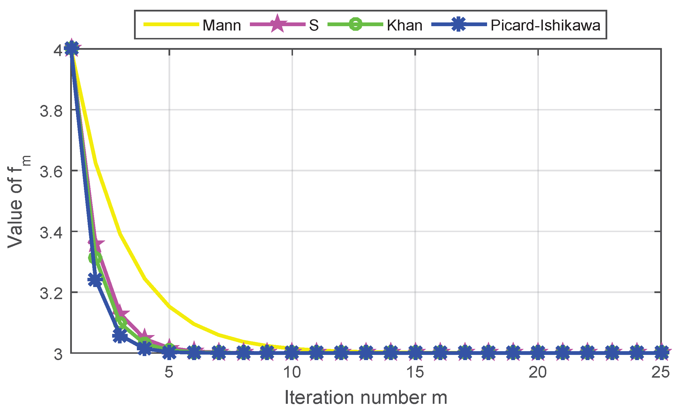
| Step | Mann | S | Khan | Picard–Ishikawa |
|---|---|---|---|---|
| 1 | 4.0000000000 | 4.0000000000 | 4.0000000000 | 4.0000000000 |
| 2 | 3.6250000000 | 3.3593750000 | 3.3125000000 | 3.2421875000 |
| 3 | 3.3906250000 | 3.1291503906 | 3.0976562500 | 3.0586547852 |
| 4 | 3.2441406250 | 3.0464134216 | 3.0305175781 | 3.0142054558 |
| 5 | 3.1525878906 | 3.0166798234 | 3.0095367432 | 3.0034403838 |
| 6 | 3.0953674316 | 3.0059943115 | 3.0029802322 | 3.0008332180 |
| 7 | 3.0596046448 | 3.0021542057 | 3.0009313226 | 3.0002017950 |
| 8 | 3.0372529030 | 3.0007741677 | 3.0002910383 | 3.0000488722 |
| 9 | 3.0232830644 | 3.0002782165 | 3.0000909495 | 3.0000118362 |
| 10 | 3.0145519152 | 3.0000999841 | 3.0000284217 | 3.0000028666 |
| 11 | 3.0090949470 | 3.0000359318 | 3.0000088818 | 3.0000006943 |
| 12 | 3.0056843419 | 3.0000129130 | 3.0000027756 | 3.0000001681 |
| 13 | 3.0035527137 | 3.0000046406 | 3.0000008674 | 3.0000000407 |
| 14 | 3.0022204460 | 3.0000016677 | 3.0000002711 | 3.0000000099 |
| 15 | 3.0013877788 | 3.0000005993 | 3.0000000847 | 3.0000000024 |
| 16 | 3.0008673617 | 3.0000002154 | 3.0000000265 | 3.0000000006 |
| 17 | 3.0005421011 | 3.0000000774 | 3.0000000083 | 3.0000000001 |
| 18 | 3.0003388132 | 3.0000000278 | 3.0000000026 | 3.0000000000 |
| 19 | 3.0002117582 | 3.0000000100 | 3.0000000008 | 3.0000000000 |
| 20 | 3.0001323489 | 3.0000000036 | 3.0000000003 | 3.0000000000 |
| 21 | 3.0000827181 | 3.0000000013 | 3.0000000001 | 3.0000000000 |
| 22 | 3.0000516988 | 3.0000000005 | 3.0000000000 | 3.0000000000 |
| 23 | 3.0000323117 | 3.0000000002 | 3.0000000000 | 3.0000000000 |
| 24 | 3.0000201948 | 3.0000000001 | 3.0000000000 | 3.0000000000 |
| 25 | 3.0000126218 | 3.0000000000 | 3.0000000000 | 3.0000000000 |
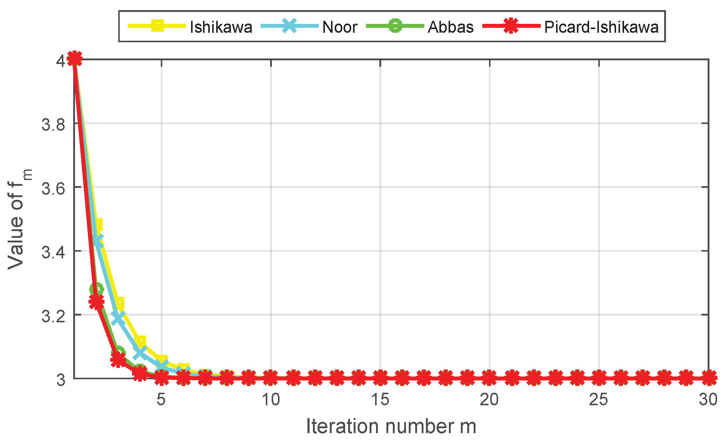
| Step | Ishikawa | Noor | Abbas | Picard–Ishikawa |
|---|---|---|---|---|
| 1 | 4.0000000000 | 4.0000000000 | 4.0000000000 | 4.0000000000 |
| 2 | 3.4843750000 | 3.4316406250 | 3.2792968750 | 3.2421875000 |
| 3 | 3.2346191406 | 3.1863136292 | 3.0780067444 | 3.0586547852 |
| 4 | 3.1136436462 | 3.0804205313 | 3.0217870399 | 3.0142054558 |
| 5 | 3.0550461411 | 3.0347127684 | 3.0060850522 | 3.0034403838 |
| 6 | 3.0266629746 | 3.0149834411 | 3.0016995361 | 3.0008332180 |
| 7 | 3.0129148783 | 3.0064674619 | 3.0004746751 | 3.0002017950 |
| 8 | 3.0062556442 | 3.0027916193 | 3.0001325753 | 3.0000488722 |
| 9 | 3.0030300777 | 3.0012049763 | 3.0000370279 | 3.0000118362 |
| 10 | 3.0014676939 | 3.0005201167 | 3.0000103418 | 3.0000028666 |
| 11 | 3.0007109142 | 3.0002245035 | 3.0000028884 | 3.0000006943 |
| 12 | 3.0003443491 | 3.0000969048 | 3.0000008067 | 3.0000001681 |
| 13 | 3.0001667941 | 3.0000418281 | 3.0000002253 | 3.0000000407 |
| 14 | 3.0000807909 | 3.0000180547 | 3.0000000629 | 3.0000000099 |
| 15 | 3.0000391331 | 3.0000077931 | 3.0000000176 | 3.0000000024 |
| 16 | 3.0000189551 | 3.0000033638 | 3.0000000049 | 3.0000000006 |
| 17 | 3.0000091814 | 3.0000014520 | 3.0000000014 | 3.0000000001 |
| 18 | 3.0000044472 | 3.0000006267 | 3.0000000004 | 3.0000000000 |
| 19 | 3.0000021541 | 3.0000002705 | 3.0000000001 | 3.0000000000 |
| 20 | 3.0000010434 | 3.0000001168 | 3.0000000000 | 3.0000000000 |
| 21 | 3.0000005054 | 3.0000000504 | 3.0000000000 | 3.0000000000 |
| 22 | 3.0000002448 | 3.0000000218 | 3.0000000000 | 3.0000000000 |
| 23 | 3.0000001186 | 3.0000000094 | 3.0000000000 | 3.0000000000 |
| 24 | 3.0000000574 | 3.0000000041 | 3.0000000000 | 3.0000000000 |
| 25 | 3.0000000278 | 3.0000000017 | 3.0000000000 | 3.0000000000 |
| 26 | 3.0000000135 | 3.0000000008 | 3.0000000000 | 3.0000000000 |
| 27 | 3.0000000065 | 3.0000000003 | 3.0000000000 | 3.0000000000 |
| 28 | 3.0000000032 | 3.0000000001 | 3.0000000000 | 3.0000000000 |
| 29 | 3.0000000015 | 3.0000000001 | 3.0000000000 | 3.0000000000 |
| 30 | 3.0000000007 | 3.0000000000 | 3.0000000000 | 3.0000000000 |
Disclaimer/Publisher’s Note: The statements, opinions and data contained in all publications are solely those of the individual author(s) and contributor(s) and not of MDPI and/or the editor(s). MDPI and/or the editor(s) disclaim responsibility for any injury to people or property resulting from any ideas, methods, instructions or products referred to in the content. |
© 2024 by the authors. Licensee MDPI, Basel, Switzerland. This article is an open access article distributed under the terms and conditions of the Creative Commons Attribution (CC BY) license (https://creativecommons.org/licenses/by/4.0/).
Share and Cite
Ugboh, J.A.; Oboyi, J.; Udo, M.O.; Nabwey, H.A.; Ofem, A.E.; Narain, O.K. On a Faster Iterative Method for Solving Fractional Delay Differential Equations in Banach Spaces. Fractal Fract. 2024, 8, 166. https://doi.org/10.3390/fractalfract8030166
Ugboh JA, Oboyi J, Udo MO, Nabwey HA, Ofem AE, Narain OK. On a Faster Iterative Method for Solving Fractional Delay Differential Equations in Banach Spaces. Fractal and Fractional. 2024; 8(3):166. https://doi.org/10.3390/fractalfract8030166
Chicago/Turabian StyleUgboh, James Abah, Joseph Oboyi, Mfon Okon Udo, Hossam A. Nabwey, Austine Efut Ofem, and Ojen Kumar Narain. 2024. "On a Faster Iterative Method for Solving Fractional Delay Differential Equations in Banach Spaces" Fractal and Fractional 8, no. 3: 166. https://doi.org/10.3390/fractalfract8030166
APA StyleUgboh, J. A., Oboyi, J., Udo, M. O., Nabwey, H. A., Ofem, A. E., & Narain, O. K. (2024). On a Faster Iterative Method for Solving Fractional Delay Differential Equations in Banach Spaces. Fractal and Fractional, 8(3), 166. https://doi.org/10.3390/fractalfract8030166