Accelerated Gradient Descent Driven by Lévy Perturbations

Abstract

In this paper, we mainly consider two kinds of perturbed accelerated gradient descents driven by Lévy perturbations, which is of great importance for enhancing the global search ability. By using Lévy representation, Lévy perturbations can be divided into two parts: small jumps and large jumps, whose properties are then carefully discussed. By introducing the concept of attraction domain for local minima, Makovian transition properties are proven for the proposed two perturbed accelerated gradient descents with different infinitesimal matrices. Finally, all the results are extended to the vector case and two simulation examples are provided to validate all the conclusions.

1. Introduction

Nowadays, optimization problems can be found almost everywhere, for instance, (1) Modeling: minimize some given cost function to find the optimal parameters for describing a system [1]; (2) Optimal control: find the optimal controller parameters for different goals, such as most energy-saving, most time-saving, or the fastest response rate [2]; (3) Machine learning: an important task of machine learning is to train the neural network to find a set of parameters that minimize the mismatching rate [3].

The key to an optimization problem is the optimization algorithm. Among all the existing optimization algorithms, gradient descent (GD) [4,5] is a basic but popular optimization algorithm and plays an important role in all kinds of problems. Moreover, to overcome the shortcomings of GD, many variants have been proposed. For instance, accelerated GDs (AGDs) including GD with momentum [6,7] and Nesterov acceleration [8], have been proposed to increase the convergence speed. Unlike AGD which is accelerated by introducing one more variable, second-order algorithms such as Newton method and quasi-Newton method [9], increase the convergence speed by modifying the iteration direction. Moreover, it has been shown that AGDs can be described by a second-order transfer function and its properties can be derived using system theory [7,10]. Some methods for estimating the Hessian matrix have also been provided to make Newton method more applicable [11,12].

As is known, GD is a local algorithm since gradient information is local, for which GD can easily fall into a local minimum point and it will be quite tough for escaping from a saddle point. To increase the global search ability of GD for non-convex optimization, perturbed GDs (PGDs) have then been proposed. The PGD driven by Brownian noise can be viewed as the discrete form of the Langevin equation in physics [13], which is used to interpret particle’s transition between different potential wells [14]. Each potential well plays the same role as an attraction domain of a local minimum point in optimization, thus PGD can help jumping out a local minimum and existing PGD driven by Brownian motion has been proven to jump out a local minimum but the first exist time depends exponentially on the depth of the well [15]. Moreover, PGD can also help escaping the saddle point and the property for faster escaping from saddle point was carefully discussed in [16,17]. To help jumping out the local minima more efficiently, the perturbation is then replaced by the Lévy perturbations, which is a heavy-tailed distribution and has been proven to be efficient in global searching for intelligent algorithms. Compared with the Brownian motion, the variance of Lévy perturbations is infinite and more frequently large jump sizes will take place, which contributes to jumping out the local minima a lot [18]. In [19,20], dedicated analyses were given to the simulated annealing driven by Lévy perturbations by dividing the Lévy perturbations into large jump sizes and small jump sizes. In [21], it is proven that the first exit time for escaping from a local minimum point driven by Lévy perturbations is polynomial.

Stochastic GD (SGD) was originally proposed to increase the training speed in deep learning, where it uses a random mini-batch instead of the whole data to generate an update [22,23]. SGD has the same format of the commonly used GDs in convex optimization and looks different from PGD, but they are the same in essence. Ref. [24] provided the detailed deduction for the relation between SGD and PGD by assuming that the error of the mini-batch gradient and the real gradient was distributed according to some distribution. Recently, in [24], it is found that the stochastic noise can be better described with a Lévy distribution. Moreover, in [25,26], it is found that the first exist time from a local minimum is only polynomial with the width of the well, which is conflict to the existing results. Thus GD driven by Lévy perturbations is then get increasing attention. In [27], the Langevin Monte Carlo driven by Lévy perturbations was carefully discussed and by carefully designing the drift item, the convergence to the invariant measure was proven. On this basis, in [28], the results were extended to the overdamped Langevin Monte Carlo, where an additional momentum item was included to accelerate the convergence speed to the invariant measure.

AGD has already been widely used in deep learning. Similar to the procedures provided in [24] where stochastic GD is reformulated as the conventional PGD, accelerated PGD (PAGD) can be derived. There have already been some work about the properties of PAGD driven by Brownian motion [29]. However, properties of PAGD driven by Lévy fligths have not been analyzed yet, which is of great importance in deep learning [24]. Therefore, in this study, two different types of PAGDs will be proposed and their corresponding continuous case will also be given. Divide Lévy perturbations into two parts: small jumps and large jumps and their properties are then carefully discussed. On this basis, by introducing the concept of attraction domain for local minima, Makovian transition properties will be proven for the proposed PAGDs with different infinitesimal matrices. Finally, two simulation examples are provided to validate all the conclusions. The main contribution of the paper is summarized as follows

• By dividing the Lévy perturbation into small jumps and large jumps, a general framework for analyzing PAGDs is given;
• Convergence performance of PAGDs are analyzed under small perturbations and large perturbations respectively;
• By introducing the concept of attraction domain for local minima, Makovian transition properties are proven for PAGDs.

2. Preliminaries

In this paper, consider the following unconstrained nonconvex optimization problem

$$\underset{x\in {\mathbb{R}}^n}{min}f\left(x\right)$$

where $f\left(x\right)$ is differentiable and has multi local minimum points ${\left\{m_i\right\}}_{i=1}^r$.

2.1. Accelerated Gradient Descent

The commonly used AGD with momentum item [10] can be formulated as

$$\left\{\begin{array}{c}{y}_{k+1}=\lambda y_k-\rho \nabla f\left(x_k\right),\hfill \\ x_{k+1}=x_k+y_{k+1},\hfill \end{array}\right.$$

(1)

and its corresponding continuous form [30] is

$$\left\{\begin{array}{c}dy=\left(\lambda -1\right)ydt-\rho \nabla f\left(x\right)dt,\hfill \\ dx=ydt,\hfill \end{array}\right.$$

(2)

where $0<\lambda <1$, $\rho >0$ is the step size, and $\nabla f\left(x_k\right)$ denotes the gradient of $f\left(x\right)$ at $x_k$. In all the following, it is assumed that $f\left(x\right)$ satisfies the following condition locally

$$\begin{array}{c}\hfill \mu \parallel x-y\parallel \le \parallel \nabla f\left(x\right)-\nabla f\left(y\right)\parallel \le L\parallel x-y\parallel ,\end{array}$$

(3)

where $\mu >0$ and $L>0$.

2.2. Perturbed Gradient Descent

The PGD can be derived by adding a perturbation item

$$x_{k+1}=x_k-\rho \nabla f\left(x_k\right)+\epsilon {\eta }_k,$$

(4)

where, $\epsilon >0$ is the scaling parameter and ${\eta }_k$ is the perturbation generated from some given distribution, such as Gaussian distribution or Lévy distribution introduced in the following. PGD has played an important role in interpreting the excellent performance of stochastic GD in machine learning, where the target function is always non-convex [24].

2.3. Stable Process and Lévy Perturbations

Lévy distribution, a symmetric unbiased stable distribution, $F\left(x\right)$ is defined by its characteristic function [31]

$$F\left(k\right)=e^{-\gamma {\left|k\right|}^{\alpha }},0<\alpha <2,$$

(5)

where $\gamma >0$ is the scaling parameter and $\alpha$ is called Lévy index.

A symmetric stable process $L_t,t\ge 0$ is a Markov process with independent stationary increments and marginal with a Lévy distribution. Stable process $L_t$ can be described by its characteristic function [32]

$$E\left\{e^{ik{L}_t}\right\}=e^{-at{\left|k\right|}^{\alpha }},0<\alpha <2,$$

(6)

where $a>0$ is the scaling parameter. The characteristic function of $L_t$ can be formulated in a integral form as

$$E\left\{e^{ik{L}_t}\right\}=exp\left\{t\underset{\mathbb{R}\setminus \left\{0\right\}}{\int }\left[e^{iky}-1-iky\mathbf{I}\left\{\left|y\right|\le 1\right\}\right]\frac{dy}{{\left|y\right|}^{1+\alpha }}\right\}.$$

(7)

where $\mathbf{I}\left\{\left|y\right|\le 1\right\}$ is the index function. It is concluded that Lévy process is a compound Poisson process and the Lévy measure of the stochastic process $L_t$ is given by

$$v\left(A\right)=\underset{A\setminus \left\{0\right\}}{\int }\frac{dy}{{\left|y\right|}^{1+\alpha }}.$$

(8)

Lemma 1

([20]). Define $d{L}_t=L_t-L_{t-}$ as the jump size of $L_t$ at time t, and the number of jumps on the time interval $(0,t]$ whose jump size belongs to the Borel set A has a Poisson distribution with mean $tv \left(A\right)$.

Remark 1.

When $\alpha =2$, Lévy distribution and stable process $L_t$ will reduce to a Gaussian distribution and Brownian motion, respectively. Ref. [18] provided simple procedures to generate random numbers according to Lévy distribution.

According to Lemma 1 and the fact that a Poisson process can be divided into several independent Poisson processes, we will divide the Lévy flights into two parts: one is the large jump size where $|d{L}_t|=|{\eta }_k|>\kappa$ and the other one is the small jump size where $|d{L}_t|=|{\eta }_k|\le \kappa$.

For the large jump size, the Lévy measure is finite and one has that

$${\beta }_{\kappa }={\int }_{\left|x\right|\ge \kappa }\frac{dy}{{\left|y\right|}^{1+\alpha }}=\frac{2}{\alpha {\kappa }^{\alpha }}.$$

(9)

Denote ${\tau }_k$ and $W_k$ as the jump arrival times and jump sizes. Then the internal-arrival times $T_k={\tau }_k-{\tau }_{k-1}$ are identically independent and exponentially distributed with mean ${\beta }_{\kappa }^{-1}$. According to the property of Poisson process, it is known that thr probability density function of ${\tau }_k$ satisfies a Gamma distribution

$$\begin{array}{c}\hfill f\left({\beta }_{\phi },k\right)=\frac{{\beta }_{\phi }{\mathrm{e}}^{-{\beta }_{\phi }t}{\left({\beta }_{\phi }t\right)}^{k-1}}{\left(k-1\right)!}.\end{array}$$

(10)

Moreover, perturbations in between two successive large step sizes are all small jump sizes (bounded by $\kappa$).

Remark 2.

The above analyses indicate that Lévy index could control both the frequency and amplitude of large jumps. The smaller Lévy index, the more frequent large jumps and the larger amplitude.

3. PAGDs Driven by Lévy Perturbations

Combining the AGD with a perturbation item, one can derive two kinds of PAGDs respectively as

$$\left\{\begin{array}{c}{y}_{k+1}=\lambda y_k-\rho \nabla f\left(x_k\right),\hfill \\ x_{k+1}=x_k+y_{k+1}+\epsilon {\eta }_k,\hfill \end{array}\right.$$

(11)

and

$$\left\{\begin{array}{c}{y}_{k+1}=\lambda y_k-\rho \nabla f\left(x_k\right)+\epsilon {\eta }_k,\hfill \\ x_{k+1}=x_k+y_{k+1}.\hfill \end{array}\right.$$

(12)

where the perturbation $\epsilon {\eta }_k$ is added to different positions.

For the convenience, the following property analyses will mainly based on their continuous forms and Lévy perturbations are used, which can be described respectively as

$$\left\{\begin{array}{c}dy=\left(\lambda -1\right)ydt-\rho \nabla f\left(x\right)dt,\hfill \\ dx=ydt+\epsilon d{L}_t,\hfill \end{array}\right.$$

(13)

and

$$\left\{\begin{array}{c}dy=\left(\lambda -1\right)ydt-\rho \nabla f\left(x\right)dt+\epsilon d{L}_t,\hfill \\ dx=ydt.\hfill \end{array}\right.$$

(14)

Remark 3.

PGD (4) is the discrete form of the overdamped Langevin equation while PAGD (14) is known as the underdamped Langevin equation. We have to mention that PAGD (11) is newly proposed in this study. One may refer the work of [30] for more details about the discrete and continuous forms of AGDs.

Remark 4.

In neural network training, stochatic GD is often used and it has been shown in [24] that the gradient estimation error can be better modeled by a Lévy perturabtion. In the following, we will focus on the property analyses of PAGDs driven by Lévy perturabtion.

Convergence Analyses for Small Perturbations

Theorem 1.

Set $\kappa ={\epsilon }^{-\gamma },0<\gamma <1$. As $\epsilon \to 0$, the trajectories of PAGDs (13) and (14) will both converge to that of AGD (2) for small perturbations bounded by κ.

Proof. 

The solution of differential Equation (2) is

$$\overline{x}\left(t\right)=x_0+{\int }_0^t\left[e^{\left(\lambda -1\right)T}{y}_0-\rho {\int }_0^T{e}^{\left(\lambda -1\right)\left(T-\tau \right)}\nabla f\left(\overline{x}\right)d\tau \right]dT,$$

(15)

and the solution of differential Equation (14) is

$$x\left(t\right)=x_0+{\int }_0^t\left[e^{\left(\lambda -1\right)T}{y}_0-\rho {\int }_0^T{e}^{\left(\lambda -1\right)\left(T-\tau \right)}\nabla f\left(x\right)d\tau \right]dT+\epsilon L_t.$$

(16)

Then the absolute error between $x\left(t\right)$ and $\overline{x}\left(t\right)$ is

$$\begin{array}{cc}\hfill \parallel \overline{x}\left(t\right)-x\left(t\right)\parallel =& \parallel \rho {\int }_0^t{\int }_0^T{e}^{\left(\lambda -1\right)\left(T-\tau \right)}\left[\nabla f\left(x\right)-\nabla f\left(\overline{x}\right)\right]d\tau dT+\epsilon L_t\parallel \hfill \\ \hfill \le & \rho L{\int }_0^t{\int }_0^T{e}^{\left(\lambda -1\right)\left(T-\tau \right)}\parallel \overline{x}\left(\tau \right)-x\left(\tau \right)\parallel d\tau dT+\parallel \epsilon L_t\parallel \hfill \\ \hfill =& \rho L{\int }_0^t\parallel \overline{x}\left(\tau \right)-x\left(\tau \right)\parallel {\int }_{\tau }^t{e}^{\left(\lambda -1\right)\left(T-\tau \right)}dTd\tau +\parallel \epsilon L_t\parallel \hfill \\ \hfill \le & \frac{\rho L}{1-\lambda }{\int }_0^t\parallel \overline{x}\left(\tau \right)-x\left(\tau \right)\parallel d\tau +\parallel \epsilon L_t\parallel ,\hfill \end{array}$$

where condition (3) is used.

As $\epsilon \to 0$, one has that $\parallel \epsilon d{L}_t\parallel \le {\epsilon }^{1-\gamma }\to 0$ and

$$\parallel \overline{x}\left(t\right)-x\left(t\right)\parallel \le \frac{\rho L}{1-\lambda }{\int }_0^t\parallel \overline{x}\left(\tau \right)-x\left(\tau \right)\parallel d\tau .$$

Using Gronwall’s inequality [33], we have that

$$\parallel \overline{x}\left(t\right)-x\left(t\right)\parallel \le 0,$$

which indicates the results of the given theorem.

For the differential Equation (14), the result still holds and the proof procedures are similar. □

Remark 5.

Theorem 1 indicates that if ε is set sufficiently small, the small perturbations (bounded by κ) will not influence the convergence trajectory a lot. In other words, small perturbations in Lévy perturbations will not enhance the global search ability while the large perturbations will do. Therefore, we will focus on the analyses on large perturbations in the following.

Assumption 1.

Set $\kappa ={\epsilon }^{-\gamma },0<\gamma <1$. As $\epsilon \to 0$, it is assumed that the mean waiting time of successive large jumps is much longer than the convergence time of AGD (2) to the ε-neighbourhood of a local minimum point i.e., $\parallel x\left(t\right)-x^{\ast }\parallel \le \epsilon$.

According to aforementioned discussion, perturbations in between two successive large jumps are all smaller than $\kappa$. Then the convergence time to a local minimum point of the conventional GD from its corresponding attraction domain could be derived. Choose Lyapunov function $V={∥x-x^{\ast }∥}^2$ and take first-order time derivative, yielding,

$$\dot{V}=-2\rho {\nabla }^{\mathrm{T}}f\left(x\right)\left(x-x^{\ast }\right)\le -2\rho \mu {∥x-x^{\ast }∥}^2=-2\rho \mu V.$$

where condition (3) is used. It is concluded that

$$\begin{array}{c}\hfill {∥x-x^{\ast }∥}^2\le {∥x_0-x^{\ast }∥}^2{\mathrm{e}}^{-2\rho \mu t}.\end{array}$$

(17)

Therefore, if $t\ge \frac{1}{2\rho \mu }ln\left(\frac{{∥x_0-x^{\ast }∥}^2}{\epsilon }\right)$, conventional GD will converge to the $\epsilon$-neighbourhood of local minimum point. Besides, the mean waiting time of two successive large jumps is $\frac{\alpha }{2{\epsilon }^{\gamma \alpha }}$. As $\epsilon \to 0$. it is concluded that $\frac{\alpha }{2{\epsilon }^{\gamma \alpha }}$ is much larger than $\frac{1}{2\rho \mu }ln\left(\frac{{∥x_0-x^{\ast }∥}^2}{\epsilon }\right)$. Since AGD converges faster than the conventional GD by carefully tuning the parameters, Assumption 1 can then be shown reasonable.

Remark 6.

Assumption 1 indicates that if ε is set sufficiently small, both PAGDs (13) and (14) will fall into a ε-neighbourhood of a local minimum point, which is important for the following analysis.

4. Convergence Properties for PAGD (13)

In this section, the properties of two PAGDs will be studied. Before moving, the attraction domain of a local minimum point must be defined. For a given target function $f\left(x\right)$, if the optimization algorithm is determined, then it can be viewed as a nonlinear feedback system, where a local minimum point is a steady equilibrium of the system. By using the definition of attraction domain in nonlinear systems, the attraction domain of a local minimum point can be defined.

Definition 1.

The attraction domain of a local minimum point $m_i$ is the collection of all the initial states such that the optimization algorithm finally converges to the local minimum point $m_i$.

For AGD (2) where $f\left(x\right)$ has multi local minimum points ${\left\{m_i\right\}}_{i=1}^r$, it has r steady equilibriums, i.e., ${\left(x,y\right)}^T={\left(m_i,0\right)}^T$ whose corresponding attraction domain are defined as ${\Omega }_i$.

4.1. Convergence Properties for PAGD (13)

In this subsection, PAGD (13) is considered, where the perturbation is added to x. Then define a new state space ${\left\{{\Omega }_i\right\}}_{i=1}^r$ and denote ${\sigma }_{ij}$ as the first time to jump from attraction domain ${\Omega }_i$ to attraction domain ${\Omega }_j$.

According to Lemma 1, it is concluded that ${(x,y)}^T$ has converged to a small neighbourhood of ${(m_i,0)}^T$ before the next large jump arrives and then the transition can be approximated by transition from ${(m_i,0)}^T$ to attraction domain ${\Omega }_j$. Then according to the the fact that the arrival of large perturbations constructs a Poisson process, the mean of ${\sigma }_{ij}$ can be calculated as

$$\begin{array}{c}\hfill \begin{array}{cc}\hfill E\left\{{\sigma }_{ij}\right\}=& {\displaystyle \sum _{k=1}^{\infty }}E\left\{{\tau }_k\right\}P\left({\sigma }_{ij}={\tau }_k\right)\hfill \\ \hfill =& {\displaystyle \sum _{k=1}^{\infty }}kE\left\{T_1\right\}P\left({\sigma }_{ij}={\tau }_k\right)\hfill \\ \hfill \approx & \frac{P\left(\left(m_i+\epsilon W_k,0\right)\in {\Omega }_j\right)}{{\beta }_{\phi }}{\displaystyle \sum _{k=1}^{\infty }}k{\left[1-P\left(\left(m_i+\epsilon W_1,0\right)\notin {\Omega }_i\right)\right]}^{k-1}\hfill \\ \hfill =& \frac{P\left(m_i+\epsilon W_1\in {\Omega }_j\right)}{{\beta }_{\phi }{P}^2\left(m_i+\epsilon W_1\notin {\Omega }_i\right)}.\hfill \end{array}\end{array}$$

(18)

where the definitions and properties of $W_k$ and ${\tau }_k$ are given in Section 2.3, and

$$\begin{array}{cc}\hfill P\left({\sigma }_{ij}={\tau }_k\right)\approx & P\left({\displaystyle \bigcap _{i=1}^{k-1}}{\left(m_i+\epsilon W_1,0\right)}^T\in {\Omega }_i,\left(m_i+\epsilon W_k,0\right)\in {\Omega }_j\right)\hfill \\ \hfill =& {\left(1-P\left(\left(m_i+\epsilon W_1,0\right)\notin {\Omega }_i\right)\right)}^{k-1}P\left(\left(m_i+\epsilon W_1,0\right)\in {\Omega }_j\right).\hfill \end{array}$$

Besides, the probability distribution function of ${\sigma }_{ij}$ can be calculated as

$$\begin{array}{c}\hfill \begin{array}{cc}\hfill P\left({\sigma }_{ij}>u\right)=& {\displaystyle \sum _{k=1}^{\infty }}P\left({\tau }_k>u\right)P\left({\sigma }_{ij}={\tau }_k\right)\hfill \\ \hfill =& {\displaystyle \sum _{k=1}^{\infty }}P\left({\tau }_k>u\right)P\left({\sigma }_{ij}={\tau }_k\right)\hfill \\ \hfill =& {\displaystyle \sum _{k=1}^{\infty }}{\int }_u^{\infty }\frac{{\beta }_{\phi }{\mathrm{e}}^{-{\beta }_{\phi }t}{\left({\beta }_{\phi }t\right)}^{k-1}}{\left(k-1\right)!}\mathrm{d}tP\left({\sigma }_{ij}={\tau }_k\right)\hfill \\ \hfill \approx & {\beta }_{\phi }P\left(\left(m_i+\epsilon W_1,0\right)\in {\Omega }_j\right){\int }_u^{\infty }{\displaystyle \sum _{k=1}^{\infty }}\frac{{\mathrm{e}}^{-{\beta }_{\phi }t}{\left({\beta }_{\phi }t\right)}^{k-1}{P}_{{\overline{\Omega }}_i}^{k-1}}{\left(k-1\right)!}\mathrm{d}t\hfill \\ \hfill =& \frac{P\left(\left(m_i+\epsilon W_1,0\right)\in {\Omega }_j\right)}{P\left({\left(m_i+\epsilon W_1,0\right)}_1\notin {\Omega }_i\right)}exp\left\{-u{\beta }_{\phi }P\left(\left(m_i+\epsilon W_1,0\right)\notin {\Omega }_i\right)\right\},\hfill \end{array}\end{array}$$

(19)

with $P_{{\overline{\Omega }}_i}=1-P\left(\left(m_i+\epsilon W_1,0\right)\notin {\Omega }_i\right)$. Equation (19) indicates that ${\sigma }_{ij}$ is approximately distributed to an exponential function with mean $E\left\{{\sigma }_{ij}\right\}$.

Theorem 2.

Set $\kappa ={\epsilon }^{-\gamma },0<\gamma <1$. As $\epsilon \to 0$, the transition of $x\left(t\right)$, the solution of PAGD (11), among the state space ${\left\{{\Omega }_i\right\}}_{i=1}^r$ constructs an approximate continuous Markov chain whose infinitesimal matrix is $Q={\left\{q_{ij}\right\}}_{i,j=1}^m$ with

$$q_{ij}:={\beta }_{\phi }P\left(\left(m_i+\epsilon W_1,0\right)\in {\Omega }_j\right),i\ne j,$$

$$q_{ii}=-\sum _{j\ne i}{q}_{ij}.$$

Proof. 

According to Theorem 1, the influence of small perturbations can be totally ignored. Moreover, according to Asssumption 1, if $x\left(t\right)$ falls into ${\Omega }_i$, it will soon converge to its corresponding equilibrium point ${(m_i,0)}^T$ before the next large jump arrives. The distribution of ${\sigma }_{ij}$ is calculated in (19), which follows a exponential distribution. On this basis, for $i\ne j$, $q_{ij}$ in infinitesimal matrix can be derived as

$$\underset{u\to 0}{lim}\frac{\mathrm{d}}{\mathrm{d}u}\left(1-P\left({\sigma }_{ij}>u\right)\right)={\beta }_{\phi }P\left(\left(m_i+\epsilon W_1,0\right)\in {\Omega }_j\right),$$

This completes the proof. □

4.2. Convergence Properties for PAGD (14)

In this subsection, PAGD (14) is considered, where the perturbation is added to y. Similar to the analyses for PAGD (14), denote ${\sigma }_{ij}$ as the first time to jump from attraction domain ${\Omega }_i$ to attraction domain ${\Omega }_j$. One can then calculate the mean of ${\sigma }_{ij}$ and probability distribution respectively as

$$\begin{array}{c}\hfill E\left\{{\sigma }_{ij}\right\}=\frac{P\left(\left(m_i,\epsilon W_1\right)\in {\Omega }_j\right)}{{\beta }_{\phi }{P}^2\left(\left(m_i,\epsilon W_1\right)\notin {\Omega }_i\right)}\end{array}$$

(20)

and

$$\begin{array}{c}\hfill P\left({\sigma }_{ij}>u\right)=\frac{P\left(\left(m_i,\epsilon W_1\right)\in {\Omega }_j\right)}{P\left(\left(m_i,\epsilon W_1\right)\notin {\Omega }_i\right)}exp\left\{-u{\beta }_{\phi }P\left(\left(m_i,\epsilon W_1\right)\notin {\Omega }_i\right)\right\}\end{array}$$

(21)

Remark 7.

The analyses for PAGD (11) and (12) are quite similar. Compare (19) and (21), it is found that the transition probability from ${(m_i,0)}^T$ to attraction domain ${\Omega }_j$ for PAGD (11) is $P\left(\left(m_i+\epsilon W_1,0\right)\in {\Omega }_j\right)$ while it is $P\left(\left(m_i,\epsilon W_1\right)\in {\Omega }_j\right)$ for PAGD (12), since the perturbations are added to different positions of PAGD (11) and (12).

Theorem 3.

Set $\kappa ={\epsilon }^{-\gamma },0<\gamma <1$. As $\epsilon \to 0$, the transition of $x\left(t\right)$, the solution of PAGD (11), among the state space ${\left\{{\Omega }_i\right\}}_{i=1}^r$ constructs an approximate continuous Markov chain whose infinitesimal matrix is $Q={\left\{q_{ij}\right\}}_{i,j=1}^m$ with

$$q_{ij}:={\beta }_{\phi }P\left(\left(m_i,\epsilon W_1\right)\in {\Omega }_j\right),i\ne j,$$

$$q_{ii}=-\sum _{j\ne i}{q}_{ij}.$$

4.3. Conclusive Remarks

• The results here can be extended to many other kinds of optimization algorithms, such as the conventional PGD driven by Lévy perturbations. Moreover, our results will be more precise than that in [19] by using the attraction domain as the state space rather than using the local minimum points.
• For conventional PGD, the attraction domain for a local minimum point of $f\left(x\right)$ is the interval constructed by its two adjacent maximum points. Then the probability of $P\left(\left(m_i+\epsilon W_1,0\right)\in {\Omega }_j\right)$ and $P\left(\left(m_i,\epsilon W_1\right)\in {\Omega }_j\right)$ can be calculated as shown in [19].
• Here, $\epsilon$ is set sufficiently small to guarantee the establishment of Theorem 1 and Assumption 1. For practical usage, one can set the small jumps as zero to derive the truncated Lévy perturbations and guarantee the establishment of Theorem 1. If $\kappa$ is chosen such that ${\beta }_{\kappa }^{-1}$ is much larger than the convergence time to a small neighbourhood of a local minimum point, then the results in Theorems 2 and 3 still hold for PAGDs driven by truncated Lévy perturbations.

5. Extensions to Vector Case

The aforementioned results only hold for scalar case. By using the vector form of Lévy process, the aforementioned analyses can be directly extended to the vector case. According to the presented heavy-tailed noise in [28], it is shown that the norm of the gradient noise is heavy-tailed. Therefore, according to Theorem 6.17 in [32], the characteristic function of the vector Lévy process can be formulated as follows

$$E\left\{e^{i〈k,L_t〉}\right\}=exp\left\{t{\int }_{{\mathbb{R}}^n\setminus \left\{0\right\}}\left[e^{i〈k,y〉}-1-i〈k,y〉\mathbf{I}\left\{∥y∥\le 1\right\}\right]v\left(dy\right)\right\}.$$

Since the norm of the gradient noise is heavy-tailed, the Lévy measure can be described as the mentioned measure (8) multiplied by an uniform direction stochastic variable, which can be formulated as

$$v\left(y\theta :y\in A,\theta \in B\right)={\int }_{\theta \in B}{\int }_{y\in A\setminus \left\{0\right\}}\frac{dy}{{\left|y\right|}^{1+\alpha }}M\left(d\theta \right),$$

and $M\left(d\theta \right)$ denotes the measure of $\theta$.

The analyses for the vector case is almost the same as the scalar case and the main difference concentrates on using $W_k{\Theta }_k$ to replace $W_k$ for the jump size, where $W_k$ and ${\Theta }_k$ are two independent stochastic variables ($W_k$ denotes the jump size and ${\Theta }_k$ denotes the jump direction) with

$$P\left(W_1\in A\right)=\frac{1}{\beta }{\int }_{y\in A\setminus \left\{0\right\}}\frac{dy}{{\left|y\right|}^{1+\alpha }}$$

and

$$P({\Theta }_k\in A)=M\left(A\right).$$

Then define ${\sigma }_{ij}$ as the first exit time from attraction domain ${\Omega }_i$ to ${\Omega }_j$ and following equations hold

$$E\left\{{\sigma }_{ij}\right\}=\frac{P\left(\left(m_i,\epsilon W_1{\Theta }_1\right)\in {\Omega }_j\right)}{\beta P^2\left(\left(m_i,\epsilon W_1{\Theta }_1\right)\notin {\Omega }_i\right)},$$

and

$$P\left({\sigma }_{ij}>u\right)=\frac{P\left(\left(m_i,\epsilon W_1{\Theta }_1\right)\in {\Omega }_j\right)}{P\left(\left(m_i,\epsilon W_1{\Theta }_1\right)\notin {\Omega }_i\right)}exp\left\{-u\beta P\left(\left(m_i,\epsilon W_1{\Theta }_1\right)\notin {\Omega }_i\right)\right\}.$$

Define a new state space ${\left\{{\Omega }_i\right\}}_{i=1}^r$ where ${\Omega }_i$ denotes the attraction domain for local minimum point $m_i$, and follow theorem for vector PAGD (14) can similarly derived.

Theorem 4.

Set $\kappa ={\epsilon }^{-\gamma },0<\gamma <1$. As $\epsilon \to 0$, the transition of $x\left(t\right)$, the solution of PAGD (14), among the state space ${\left\{{\Omega }_i\right\}}_{i=1}^r$ constructs an approximate continuous Markov chain whose infinitesimal matrix is $Q={\left\{q_{ij}\right\}}_{i,j=1}^m$ with

$$q_{ij}:={\beta }_{\kappa }P\left(\left(m_i,\epsilon W_1{\Theta }_1\right)\in {\Omega }_j\right),i\ne j,$$

$$q_{ii}=-\sum _{j\ne i}{q}_{ij}.$$

Furthermore, the transition property for PAGD (13) can be similarly derived as follows.

Theorem 5.

Set $\kappa ={\epsilon }^{-\gamma },0<\gamma <1$. As $\epsilon \to 0$, the transition of $x\left(t\right)$, the solution of PGD (13), among the state space ${\left\{{\Omega }_i\right\}}_{i=1}^r$ constructs an approximate continuous Markov chain whose infinitesimal matrix is $Q={\left\{q_{ij}\right\}}_{i,j=1}^m$ with

$$q_{ij}:={\beta }_{\kappa }P\left((m_i+\epsilon W_1{\Theta }_1,0)\in {\Omega }_j\right),i\ne j,$$

$$q_{ii}=-\sum _{j\ne i}{q}_{ij}.$$

Remark 8.

Compared with the scalar case, the convergence property performs almost the same, where the main difference is a direction variable Θ is introduced. Moreover, the large jump size can help jumping out a local minimum point, which can be viewed as re-initialization. We have to declare the proposed expression can better captured the characteristic of the gradient noise since it has been shown that the norm of the gradient noise is heavy-tailed in [28].

6. Illustrative Examples

In this section, some simulation examples are provided to validate all the conclusions.

Example 1.

Consider function with two local minima, which is formulated as

$$f\left(x\right)=x^2-10cos\left(x\right).$$

(22)

Set the Lévy index $\alpha =1.5$, step size $\rho =0.01$, scaling parameter $\epsilon =0.01$, and $\lambda =0.8$. Results are shown in Figure 1 and Figure 2, where case 1 and case 2 indicates using PAGD (11) and PAGD (12) respectively. Then we have the following observations

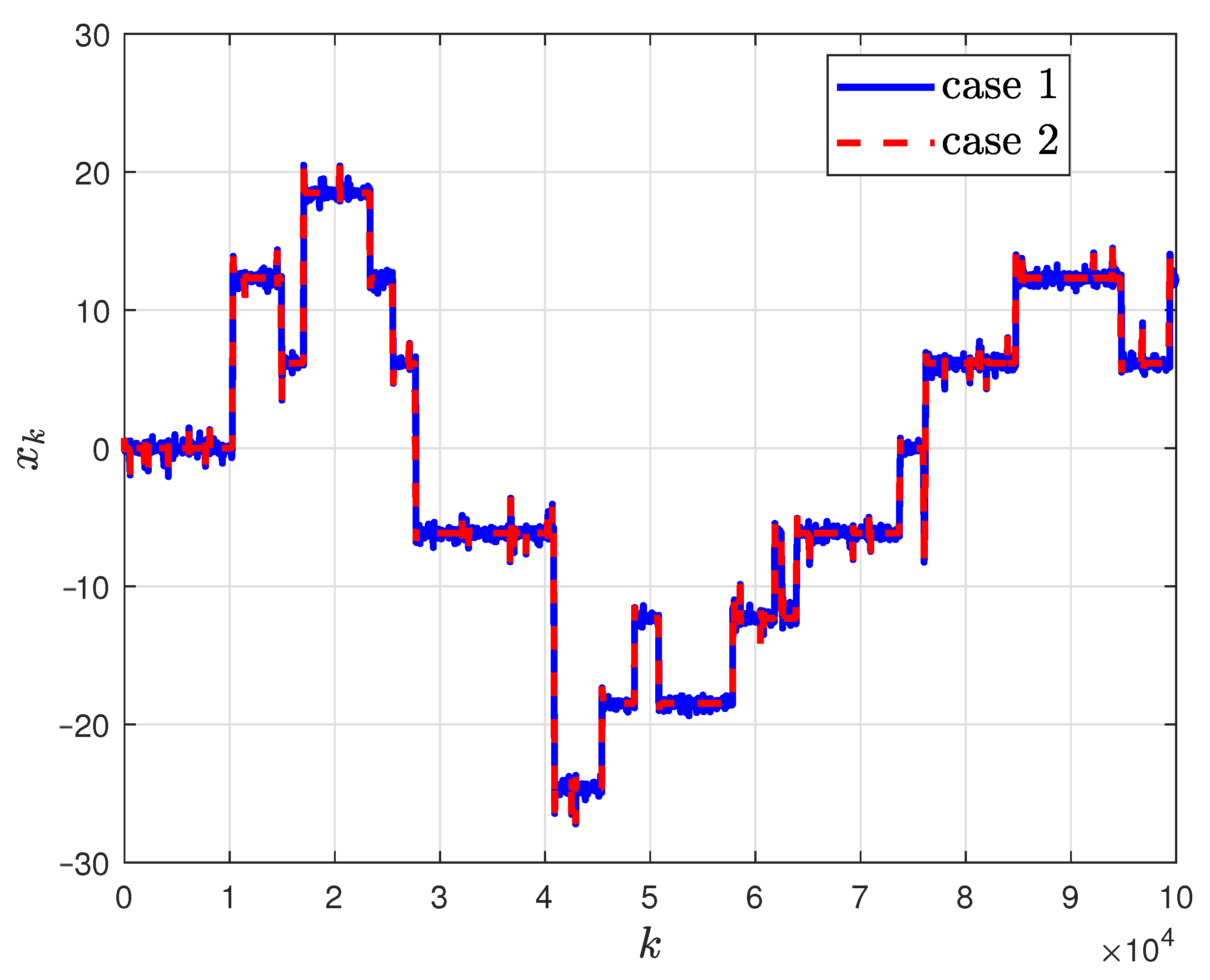
• The transition among different local minima always happens when the large jump arrives, and we have labeled some typical transition points in Figure 2, which shows the main contribution of large jumps for improving global search ability.
• For different PAGDs where perturbations are added to different positions, different transitions can be viewed with the same perturbations, where we have also labeled in Figure 2.
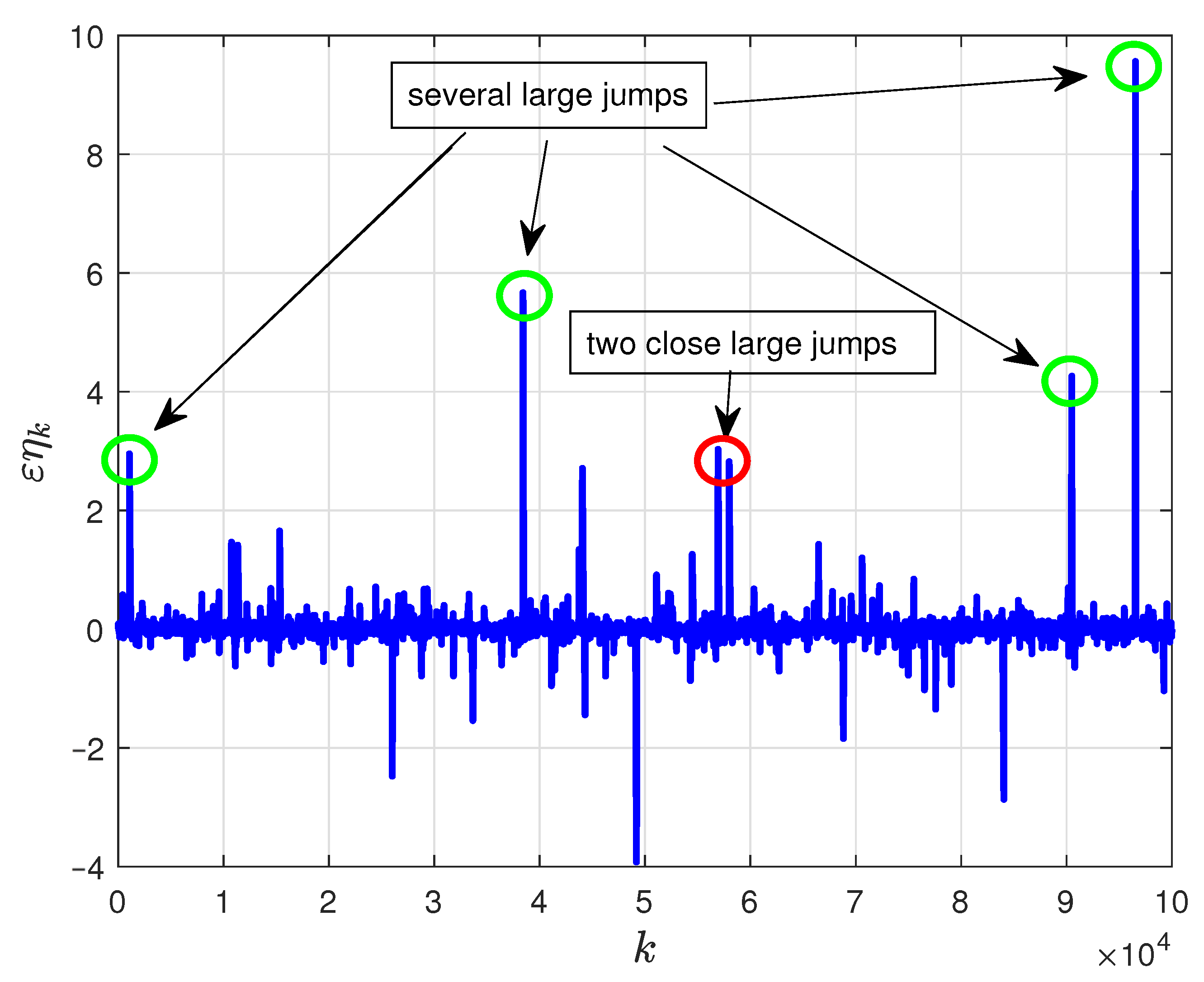
• As labeled in Figure 1, the arrival time of two successive large jumps can be very close. Therefore, Assumption 1 only holds in the mean of expectation and we can try to design the arrival time of large jumps in the future.

Figure 1. Lévy perturbations with order $\alpha =1.5$.

Figure 1. Lévy perturbations with order $\alpha =1.5$.

Figure 2. Comparison of PAGD (11) and PAGD (12).

Figure 2. Comparison of PAGD (11) and PAGD (12).

Example 2.

In this example, we will compare results of PAGD (11) driven by Lévy perturbations and truncated Lévy perturbations. Consider function with multi local minima, which is formulated as

$$f\left(x\right)=x^2-100cos\left(x\right).$$

(23)

All the parameters are the same as in Example 1. The truncated Lévy perturbations are derived by truncating Lévy perturbations with $\kappa =50$. Results are shown in Figure 3 and Figure 4, where case 1 and case 2 indicates using PAGD Lévy perturbations and truncated Lévy perturbations respectively.

• Figure 3 shows the comparison of Lévy perturbations and truncated Lévy perturbations (red circles) with threshold $\kappa =50$. Moreover, it is found that transition among local minimum points always happens when the large jump arrives, and Markovian transition property can also be observed.
• Figure 4 shows that PAGD using truncated Lévy perturbations has almost the same transitions as PAGD using Lévy perturbations. Besides, PAGD (11) using truncated Lévy perturbations has a more convergence accuracy since it has no small perturbations.

Figure 3. Lévy perturbations and truncated Lévy perturbations.

Figure 3. Lévy perturbations and truncated Lévy perturbations.

Figure 4. Comparison of PAGD (11) and truncated PAGD (11).

Figure 4. Comparison of PAGD (11) and truncated PAGD (11).

Remark 9.

The simulation results implies that the transitions always happen when the large jumps occure. In neural network training, a sudden performance improvement or deterioration is often found, where the algorithm jumps from a local minimum point to another one.

7. Conclusions and Future Topics

In this study, we have presented two types of PAGDs driven by Lévy flights and analyzed their properties. By dividing Lévy perturbations into small perturbations and large perturbations, the properties of Lévy perturbations are then carefully analyzed. On this basis, the Markovian transition properties for different PAGDs are given by introducing the concept of attraction domain for local minima. The main difference for different PAGDs is concentrated on different infinitesimal matrices. All the conclusions are finally validated by simulation examples. Some promising research topics are listed as follows

• extend the results to PAGDs with adaptive Lévy index for better convergence performance;
• extend the results to the optimization algorithms driven by truncated Lévy perturbations;
• apply the proposed PAGDs in non-convex optimization problems such as neural networks training.

References

1. Chen, Y.; Wei, Y.; Liang, S.; Wang, Y. Indirect model reference adaptive control for a class of fractional order systems. Commun. Nonlinear Sci. Numer. Simul. 2016, 39, 458–471. [Google Scholar] [CrossRef]
2. Lewis, F.L.; Vrabie, D.; Syrmos, V.L. Optimal Control; John Wiley & Sons: Hoboken, NJ, USA, 2012. [Google Scholar]
3. Witten, I.H.; Frank, E.; Hall, M.A.; Pal, C.J. Data Mining: Practical Machine Learning Tools and Techniques; Morgan Kaufmann: Amsterdam, The Netherlands, 2016. [Google Scholar]
4. Boyd, S.; Vandenberghe, L. Convex Optimization; Cambridge University Press: New York, USA, 2004. [Google Scholar]
5. Ruder, S. An overview of gradient descent optimization algorithms. arXiv 2016, arXiv:1609.04747. [Google Scholar]
6. Qian, N. On the momentum term in gradient descent learning algorithms. Neural Netw. 1999, 12, 145–151. [Google Scholar] [CrossRef]
7. Wilson, A.C.; Recht, B.; Jordan, M.I. A Lyapunov analysis of momentum methods in optimization. arXiv 2016, arXiv:1611.02635. [Google Scholar]
8. Nesterov, Y.E. A method for solving the convex programming problem with convergence rate O (1/kˆ2). Dokl. Akad. Nauk SSSR 1983, 269, 543–547. [Google Scholar]
9. Gill, P.E.; Murray, W. Quasi-Newton methods for unconstrained optimization. IMA J. Appl. Math. 1972, 9, 91–108. [Google Scholar] [CrossRef]
10. An, W.; Wang, H.; Sun, Q.; Xu, J.; Dai, Q.; Zhang, L. A PID controller approach for stochastic optimization of deep networks. In Proceedings of the IEEE Conference on Computer Vision and Pattern Recognition, Salt Lake City, UT, USA, 18–23 June 2018; pp. 8522–8531. [Google Scholar]
11. Liu, L.; Liu, X.; Hsieh, C.J.; Tao, D. Stochastic second-order methods for non-convex optimization with inexact Hessian and gradient. arXiv 2018, arXiv:1809.09853. [Google Scholar]
12. Prashanth, L.; Bhatnagar, S.; Bhavsar, N.; Fu, M.C.; Marcus, S. Random directions stochastic approximation with deterministic perturbations. IEEE Trans. Autom. Control. 2019, 65, 2450–2465. [Google Scholar] [CrossRef]
13. Stariolo, D.A. The Langevin and Fokker-Planck equations in the framework of a generalized statistical mechanics. Phys. Lett. A 1994, 185, 262–264. [Google Scholar] [CrossRef]
14. Kalmykov, Y.P.; Coffey, W.; Waldron, J. Exact analytic solution for the correlation time of a Brownian particle in a double-well potential from the Langevin equation. J. Chem. Phys. 1996, 105, 2112–2118. [Google Scholar] [CrossRef]
15. Visscher, P.B. Escape rate for a Brownian particle in a potential well. Phys. Rev. B 1976, 13, 3272. [Google Scholar] [CrossRef]
16. Jin, C.; Ge, R.; Netrapalli, P.; Kakade, S.M.; Jordan, M.I. How to escape saddle points efficiently. In Proceedings of the International Conference on Machine Learning PMLR, Sydney, Australia, 6–11 August 2017; pp. 1724–1732. [Google Scholar]
17. Staib, M.; Reddi, S.; Kale, S.; Kumar, S.; Sra, S. Escaping saddle points with adaptive gradient methods. In Proceedings of the International Conference on Machine Learning PMLR, Long Beach, CA, USA, 9–15 June 2019; pp. 5956–5965. [Google Scholar]
18. Mantegna, R.N. Fast, accurate algorithm for numerical simulation of Lévy stable stochastic processes. Phys. Rev. E 1994, 49, 4677. [Google Scholar] [CrossRef] [PubMed]
19. Imkeller, P.; Pavlyukevich, I. Lévy flights: Transitions and meta-stability. J. Phys. A Math. Gen. 2006, 39, L237. [Google Scholar] [CrossRef]
20. Pavlyukevich, I. Lévy flights, non-local search and simulated annealing. J. Comput. Phys. 2007, 226, 1830–1844. [Google Scholar] [CrossRef]
21. Imkeller, P.; Pavlyukevich, I.; Wetzel, T. The hierarchy of exit times of Lévy-driven Langevin equations. Eur. Phys. J. Spec. Top. 2010, 191, 211–222. [Google Scholar] [CrossRef]
22. Bottou, L. Large-scale machine learning with stochastic gradient descent. In Proceedings of COMPSTAT’2010; Springer: Berlin/Heidelberg, Germany, 2010; pp. 177–186. [Google Scholar]
23. Shamir, O.; Zhang, T. Stochastic gradient descent for non-smooth optimization: Convergence results and optimal averaging schemes. In Proceedings of the International Conference on Machine Learning, Miami, FL, USA, 4–7 December 2013; pp. 71–79. [Google Scholar]
24. Simsekli, U.; Sagun, L.; Gurbuzbalaban, M. A tail-index analysis of stochastic gradient noise in deep neural networks. arXiv 2019, arXiv:1901.06053. [Google Scholar]
25. Tzen, B.; Liang, T.; Raginsky, M. Local optimality and generalization guarantees for the langevin algorithm via empirical metastability. In Proceedings of the Conference on Learning Theory PMLR, Stockholm, Sweden, 6–9 July 2018; pp. 857–875. [Google Scholar]
26. Zhang, Y.; Liang, P.; Charikar, M. A hitting time analysis of stochastic gradient langevin dynamics. In Proceedings of the Conference on Learning Theory PMLR, Amsterdam, The Netherlands, 7–10 June 2017; pp. 1980–2022. [Google Scholar]
27. Nguyen, T.H.; Simsekli, U.; Richard, G. Non-asymptotic analysis of Fractional Langevin Monte Carlo for non-convex optimization. In Proceedings of the International Conference on Machine Learning PMLR, Long Beach, CA, USA, 9–15 June 2019; pp. 4810–4819. [Google Scholar]
28. Simsekli, U.; Zhu, L.; Teh, Y.W.; Gurbuzbalaban, M. Fractional underdamped langevin dynamics: Retargeting sgd with momentum under heavy-tailed gradient noise. In Proceedings of the International Conference on Machine Learning PMLR, Virtual, 13–18 June 2020; pp. 8970–8980. [Google Scholar]
29. Cheng, X.; Chatterji, N.S.; Bartlett, P.L.; Jordan, M.I. Underdamped Langevin MCMC: A non-asymptotic analysis. arXiv 2017, arXiv:1707.03663. [Google Scholar]
30. Li, Q.; Tai, C.; Weinan, E. Dynamics of stochastic gradient algorithms. arXiv 2015, arXiv:1511.06251. [Google Scholar]
31. Samoradnitsky, G. Stable Non-Gaussian Random Processes: Stochastic Models with Infinite Variance; Routledge: New York, NY, USA, 2017. [Google Scholar]
32. Meerschaert, M.M.; Sikorskii, A. Stochastic Models for Fractional Calculus; Walter de Gruyter: Berlin, Germany, 2011; Volume 43. [Google Scholar]
33. Ye, H.; Gao, J.; Ding, Y. A generalized Gronwall inequality and its application to a fractional differential equation. J. Math. Anal. Appl. 2007, 328, 1075–1081. [Google Scholar] [CrossRef]
Disclaimer/Publisher’s Note: The statements, opinions and data contained in all publications are solely those of the individual author(s) and contributor(s) and not of MDPI and/or the editor(s). MDPI and/or the editor(s) disclaim responsibility for any injury to people or property resulting from any ideas, methods, instructions or products referred to in the content.