Identification of the Dynamic Trade Relationship between China and the United States Using the Quantile Grey Lotka–Volterra Model

Abstract

The quantile regression technique is introduced into the Lotka–Volterra ecosystem analysis framework. The quantile grey Lotka–Volterra model is established to reveal the dynamic trade relationship between China and the United States. An optimisation model is constructed to solve optimum quantile parameters. The empirical results show that the quantile grey Lotka–Volterra model shows higher fitting accuracy and reveals the trade relationships at different quantiles based on quarterly data on China–US trade from 1999 to 2019. The long-term China–US trade relationship presents a prominent predator–prey relationship because exports from China to the US inhibited China’s imports from the United States. Moreover, we divide samples into five stages according to four key events, China’s accession to the WTO, the 2008 global financial crisis, the weak global economic recovery in 2015, and the 2018 China–US trade war, recognising various characteristics at different stages.

1. Introduction

1.1. Motivation

In recent years, China–US trade frictions have emerged one after another, causing adverse effects on the two largest economies: those of the United States and China. Since the China–US trade conflict officially broke out in April 2018, the trade relationship between China and the US has aroused widespread concern and discussion. According to statistics from the US Bureau of Economic Analysis (www.bea.doc.gov, accessed on 2 February 2024), the average annual growth rates of China’s total import and export volume, export scale, import scale, and trade surplus with the United States from 1999 to 2023 were 11.37%, 11.82%, 10.42%, and 8.11%, respectively. The total import and export volume and export and import scales of China–US trade were on the uptrend: the trade surplus generally expanded until the China–US trade war in 2018, after which the trade surplus shrank.

Reviewing the development history of China–US trade, since China joined WTO, its foreign trade has entered a period of significant growth, the trade relations between them have continued to deepen, and the surplus has increased rapidly. After that, the world underwent a financial crisis. In 2009, China’s foreign trade was affected by this financial crisis. The total volume of imports and exports to the United States, the scale of imports, and the trade surplus decreased by 9.72%, 12.29% and 16.55% compared with that in 2008, respectively, while China’s export trade to the United States decreased by 5.78% compared with previous years. Since 2015, the world economy has entered a period of weak recovery. Under pressure from sluggish external demand and the slow recovery of the world economy in 2015 and 2016, China’s trade scale with the United States decreased, while the gap in China’s trade surplus with the US constantly increased. Until the China–US trade war broke out in 2018, the issue of China–US trade imbalances became increasingly prominent. The trade surplus dropped from USD 378.758 billion in 2018 to USD 307.841 billion in 2019, decreasing by 18.72%. These abnormal fluctuations increased uncertainty in the development of trade relations.

To characterise the dynamic trade relationship between China and the US more accurately and then guide the healthy development of the China–US trade partnership, it is necessary to establish a reasonable model to analyse the evolution of the dynamic relationship between China and the US, thus offering practical and instructive suggestions guiding national decision making and global development.

1.2. Literature Review

A country’s international trade is closely related to its economic development; constantly increasing production demands a constantly expanding market in international trade. In other words, constantly increasing international trade can promote the continuous expansion of production. Many scholars have analysed trade relations among countries; for example, Jiang et al. [1] explored dynamic synergies between the oil market and stock markets, testing the causality of the existence of these by using wavelet multi-scale decomposition. Mahmood et al. [2] assessed the environmental effects of revenue, imports and exports, and energy consumption in five North African countries, showing exports’ adverse effects on CO₂ based on spatial panel data. However, that research was based on analysing the relationship between market-influencing factors and cannot explain dispersal behaviour or mechanisms in a mutual market. In foreign trade, frictions are inevitable among countries: how to analyse the evolution of China–US trade relations and predict future dynamic trends is an important research topic. China’s trade relations affect economic growth and social stability among countries, and at present, the academic community has not investigated dynamic trade relationships and the evolution of imports and exports.

The Lotka–Volterra model, abbreviated as the LV model, is a differential dynamic equation proposed by Lotka and Volterra [3,4]; it was initially applied to the dynamic competition among populations in the ecosystem. There are many models applied in describing the spread of species, for example, the Gompertz model [5], the logistic model [6,7], and the Bass model [8] were used to describe the spread of a species; these above models only describe the dynamic changes in a single species in a single population, ignoring information exchange between species. The LV model has been extended to many cases in recent years, such as market competition [9,10], global dynamics of a class of n-dimensional Lotka Volterra systems [11], the bank system [12], and energy and environment [13], for the model focussing on the interactions generated in an environment.

The LV model performs well in predicting the evolution of two or even multiple populations [14,15]. By comparing the advantages and disadvantages of the logistic growth model and the LV model, Modis [16] pointed out that the LV model used cross items and a couple of constant terms to promote the logistic-style growth of two or even more species. The model described the competition among individuals of the same species and how another species affects the rate at which it grows. Chiang [17] analysed dynamic competitive relationships of different types of silicon chip counterparts by constructing a novel LV model, believing that the model offers advantages in predicting the role of competitive products. Hung et al. [18] constructed a modified LV model to better predict the retail industry in Taiwan affected by seasonal and cyclical factors. Agrrawal et al. [19] determined the migration of exchange-traded fund (ETF) liquidity and its factor constituents in the US. Ditzen [20] estimated the convergence of 93 countries from 1960 to 2007 using the general Lotka–Volterra model.

Furthermore, many scholars improved the LV model from different perspectives. Marasco et al. [21] believed that the traditional LV model is flawed in assuming constant interaction coefficients and proposed a nonautonomous LV model to predict market evolution. Using statistical methods to estimate the parameters of the LV model requires large sample sizes to obtain more effective estimation results; in most cases, the available data are sparse. To solve this problem, Li et al. [22] first proposed the grey Lotka–Volterra model, abbreviated as the GLV model, based on the grey system theory [23]. In addition, Wu et al. and Gatabazi et al. [24,25] proved that a GLV model can recognise the dynamic relationship among variables compared with the traditional model. Hung et al. [26] established a combined time series method and LV model considering seasonal factors, revealing predator–prey relationships of convenience-oriented and budget-oriented forms. Zhang et al. [27] verified the random nonautonomous LV model’s random persistence and extinction problems with impulse perturbation via numerical simulation. Amore and Francisco [28] applied the Lindstedt–Poincaré method to the Lotka–Volterra model. Shi and Yan [29] studied a Lotka–Volterra competition model consisting of two equations and established an iterative algorithm and error estimation to solve the model. Zhao et al. [30] proposed a heterogeneous grey model for carbon emission prediction in 30 provinces in China.

Some scholars used non-linear least squares methods to estimate the discrete LV models [31], but these depend on initial value conditions, which readily lead to significant errors. Generally, the minimum mean absolute percentage error (MAPE) was used to compare the performance of comparative prediction models [32]. However, the minimisation principle of the MAPE had an absolute value, which caused the objective function to be non-differentiable [33]. Under the minimum MAPE principle, the non-linear grey Bernoulli model parameters were estimated in the particle swarm optimised (PSO) algorithm. Automation algorithms were deployed by Agrrawal [34] to derive capital market information. Wang and Hsu [35] estimated the parameters of the GM(1,1) model used with genetic algorithms. Wu and Wang [36] estimated the parameters in the linear regression method of the LV Model based on minimum MAPE, which performed forecast modelling for several typical macroeconomic indicators in China.

Whether using non-linear least squares or linear programming methods based on minimum MAPE, the problem of outlier-induced interference in estimation and robustness cannot be overcome effectively. Wang and Jv [37] found that the use of quantile regression based on grey system theory had a prominent optimised effect on data series with outliers. For this reason, the quantile regression technique is adopted to estimate the parameters of the non-linear GLV model in our study, and the quantile grey Lotka–Volterra model, abbreviated as the QGLV model, is proposed to reveal the dynamic relationship and evolution process among populations.

1.3. Contribution and Organization

The main contributions of this research can be summarised as follows:

(1)

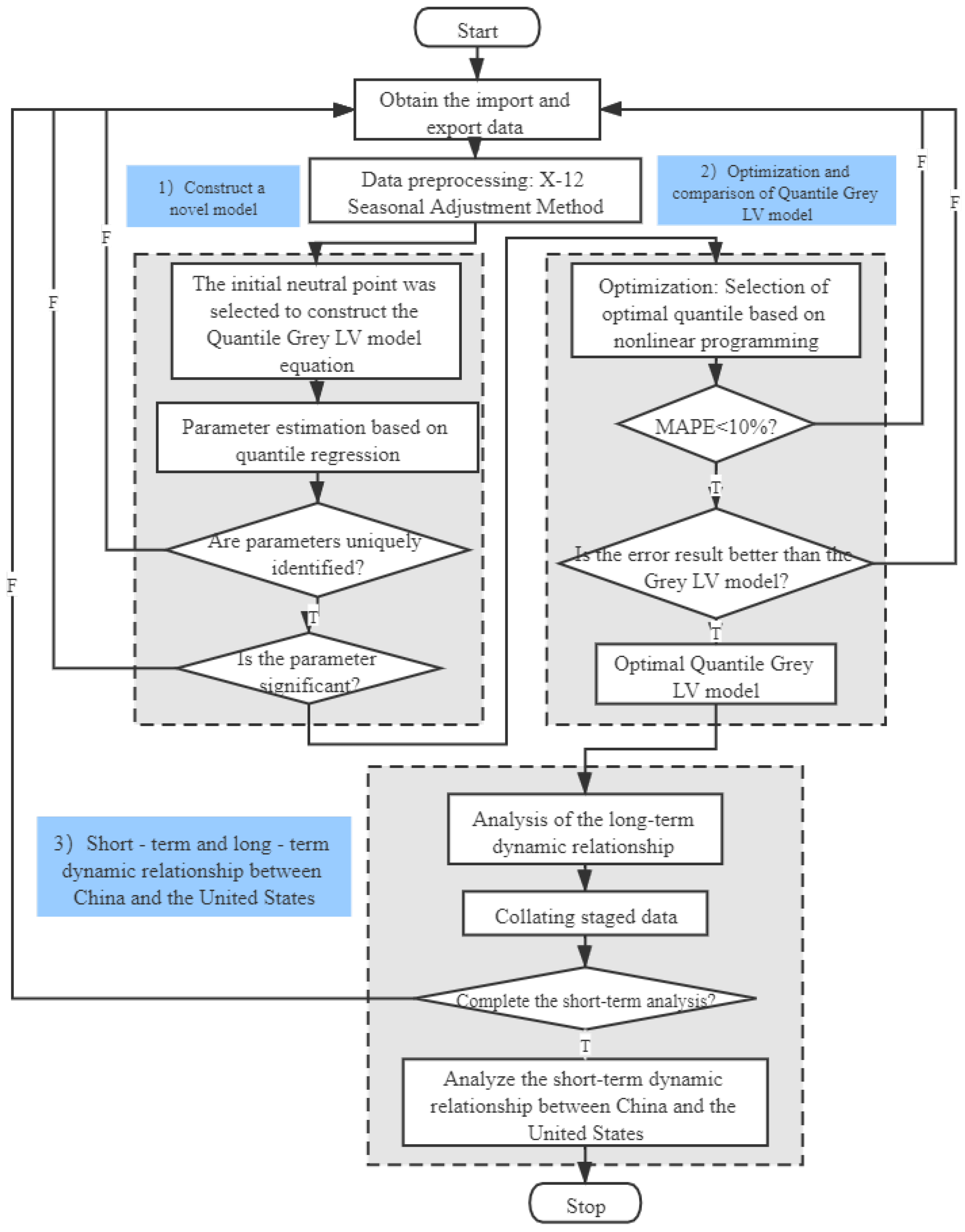
This work proposes using the quantile grey Lotka–Volterra (QGLV) model to identify the dynamic competitive relationship between the two populations. An optimization model is established based on the new model to solve the optimal quantile parameters.

(2)

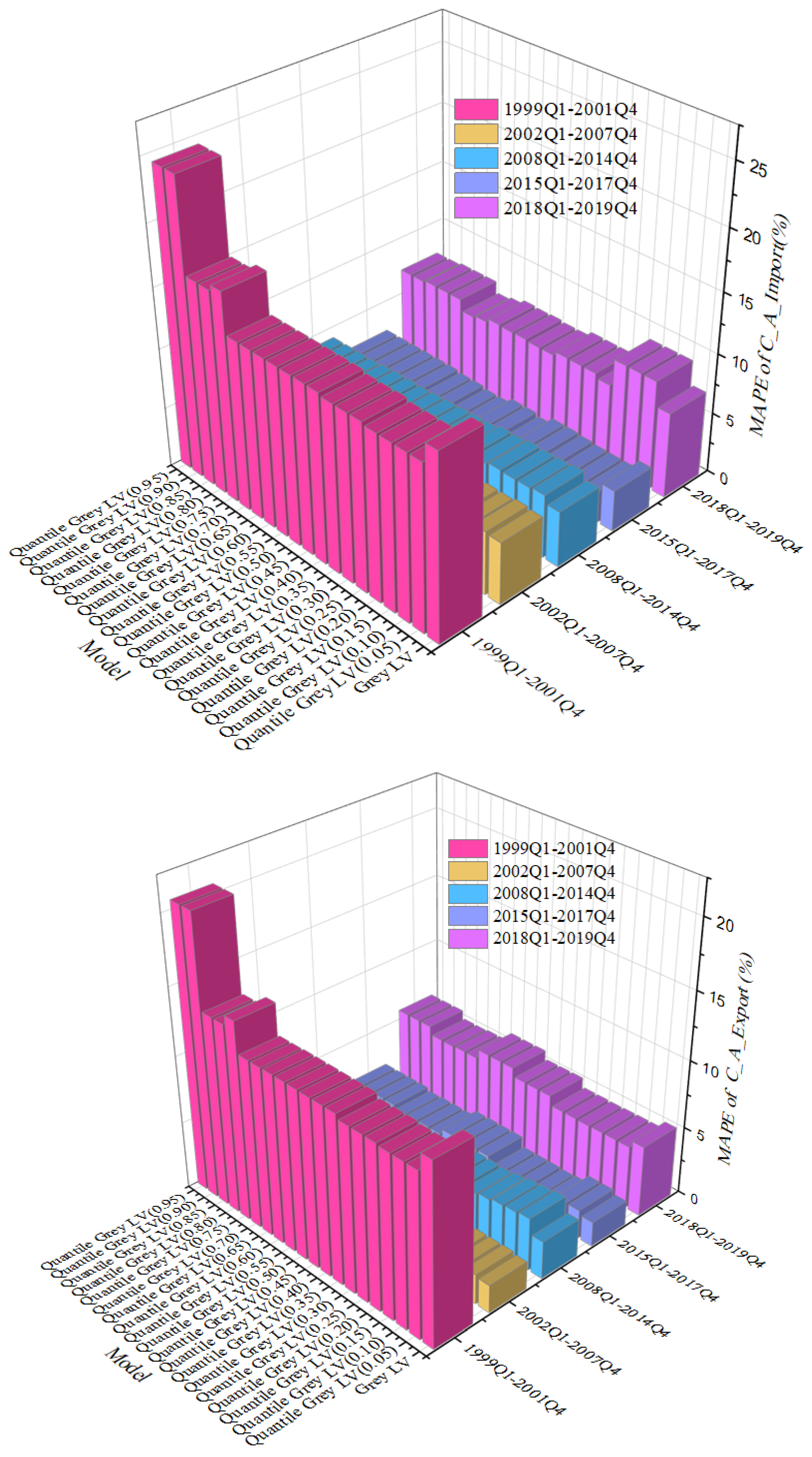
Empirical results show that the QGLV model has higher fitting accuracy than the traditional model and reveals the trade relationships at different quantiles based on quarterly data on China–US trade from 1999 to 2019.

(3)

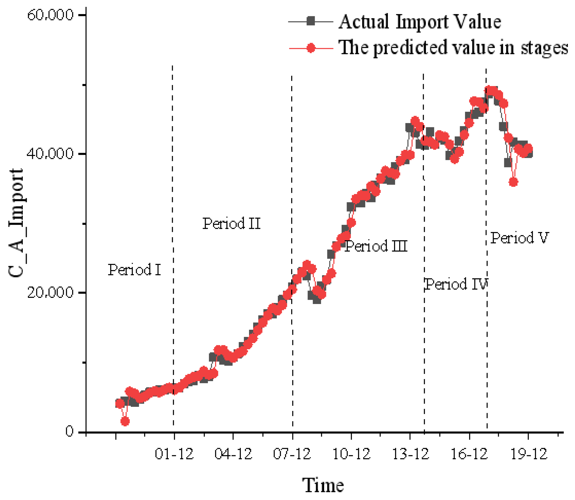
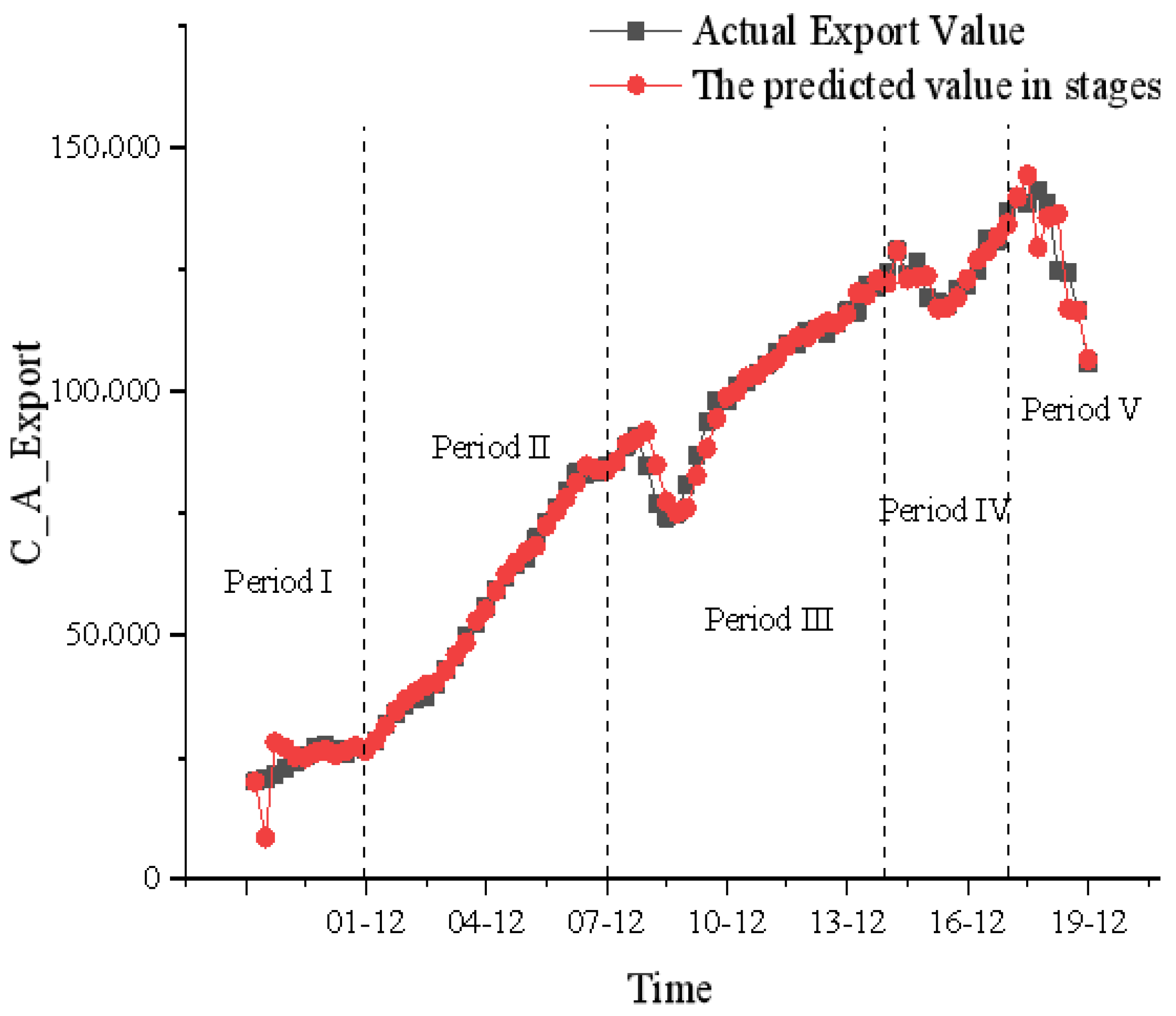
The long-term China–US trade relationship exhibits a prominent predator–prey relationship. Moreover, we divide samples into five stages according to four key events, China’s accession to the WTO, the 2008 global financial crisis, the weak global economic recovery in 2015, and the 2018 China–US trade war, recognizing variation characteristics at different stages.

The remainder of the research is arranged as follows: Section 2 presents the existing LV and the proposed QGLV models’ methods. Section 3 presents modelling results and identifies the dynamic trade relationship between China and the US. The conclusion is summarised in Section 4.

2. Methodology

The China–US trade balance is not a problem between China and the US but a global problem. China–US trade competition and cooperation relationship are dynamic and changing. Many factors can change the trade landscape between China and the United States, such as China’s accession to the WTO, the China–US trade war, and changes in the global economy. The relationship between China and the United States is no longer “black and white” but co-exists between cooperation and competition, and both sides are still exploring how to get along. In order to better describe and predict this process, we propose a new GLV model (the quantile grey Lotka–Volterra model, the QGLV model) to assess the China–US trade relations with its traditional counterpart and verify the validity of the QGLV model.

2.1. The Existing GLV Model

The Lotka–Volterra model was first used to describe the competition or symbiotic relationship among ecological populations, which is one of the differential dynamic models based on the logistic curve. As the LV model considers the influence of different populations, it has more advantages than the logistic model in describing the changes in a single variable. Taking two populations, for example, the traditional LV model [38] can be expressed as follows:

$$\frac{dA}{dt}=A(a_1-b_{1}A-c_{1}B)=a_{1}A-b_1{A}^2-c_{1}AB$$

(1)

$$\frac{dB}{dt}=B(a_2-b_{2}B-c_{2}A)=a_{2}B-b_2{B}^2-c_{2}BA$$

(2)

where $A$ and $B$ represent the volume of China’s import trade to the US and China’s export trade to the US, respectively. Taking Equation (1) as an example, $a_1$ is an exponential growth parameter, indicating the impact of China’s ability to import from the United States on its further development; $b_1$ is a self-limiting parameter, demonstrating the fact that China’s import capacity to the United States is limited; $c_1$ is coupling strength of the interaction between import and export of China–US trade, showing that there is a cross-impact between the value of China’s imports and exports to the US. Equation (2) is of a similar form; $c_1$ and $c_2$ are two kernel parameters in Equations (1) and (2), theoretically. The larger the absolute values of $c_1$ and $c_2$, the more frequent the interaction among populations and the smoother the exchange of information between populations.

Most data are discrete, and when using discrete data, it is necessary to transform Equations (1) and (2) to discretise the LV model [39].

$$\alpha (\kappa +1)=\frac{{\lambda }_1\alpha (\kappa )}{1+{\theta }_1\alpha (\kappa )+{\gamma }_1\beta (\kappa )},\kappa =1,2,\dots ,n$$

(3)

$$\beta (\kappa +1)=\frac{{\lambda }_2\beta (\kappa )}{1+{\theta }_2\beta (\kappa )+{\gamma }_2\alpha (\kappa )},\kappa =1,2,\dots ,n$$

(4)

During discretisation transforming Equations (1) and (2) to Equations (3) and (4), the corresponding relationship of each parameter is as follows:

$$a_1=\ln {\lambda }_1,a_2=\ln {\lambda }_2; b_1=\frac{{\theta }_1\ln {\lambda }_1}{{\lambda }_1-1}, b_2=\frac{{\theta }_2\ln {\lambda }_2}{{\lambda }_2-1}; c_1=\frac{{\gamma }_1\ln {\lambda }_1}{{\lambda }_1-1}, c_2=\frac{{\gamma }_2\ln {\lambda }_2}{{\lambda }_2-1}.$$

Since the data sample size is small in practical problems, the parameter could not be estimated by the classical regression estimation method effectively. Using the grey system theory to estimate the parameters in the LV model has been proven to be effective. Firstly, two non-negative original sequences are assumed to be

$$A^{(0)}=\left\{{\alpha }^{(0)}(1),{\alpha }^{(0)}(2),\dots ,{\alpha }^{(0)}(n)\right\}$$

(5)

$$B^{(0)}=\left\{{\beta }^{(0)}(1),{\beta }^{(0)}(2),\dots ,{\beta }^{(0)}(n)\right\}$$

(6)

Using the first order accumulated generating sequence (1-AGO) of $A^{(0)}$ and $B^{(0)}$, the following can be obtained:

$$A^{(1)}=\left\{{\alpha }^{(1)}(1),{\alpha }^{(1)}(2),\dots ,{\alpha }^{(1)}(n)\right\}$$

(7)

$$B^{(1)}=\left\{{\beta }^{(1)}(1),{\beta }^{(1)}(2),\dots ,{\beta }^{(1)}(n)\right\}$$

(8)

where each accumulative value is ${\alpha }^{(1)}(\kappa )={\displaystyle \sum _{i=1}^{\kappa }{\alpha }^{(0)}(i)}$, ${\beta }^{(1)}(\kappa )={\displaystyle \sum _{i=1}^{\kappa }{\beta }^{(0)}(i)}$, $\kappa =1,2\dots ,n.$

Taking ${\alpha }^{(0)}$ as an example, the grey differential equation is supposed to be $\frac{d{\alpha }^{(1)}}{dt}+a{\alpha }^{(1)}=b$; then, the discrete grey differential equation can be expressed as

$$\frac{d{\alpha }^{(1)}}{dt}=\frac{{\alpha }^{(1)}(\kappa +\mathrm{\Delta }t)-{\alpha }^{(1)}(\kappa )}{\mathrm{\Delta }t}\approx {\alpha }^{(1)}(\kappa +1)-{\alpha }^{(1)}(\kappa )={\alpha }^{(0)}(\kappa )$$

(9)

where $\mathrm{\Delta }t=1$. Close neighbour average values of cumulative sequences of ${\alpha }^{(1)}$ and ${\beta }^{(1)}$ are

$${\phi }_{\alpha }^{(1)}(\kappa )=\frac{{\alpha }^{(1)}(\kappa )+{\alpha }^{(1)}(\kappa +1)}{2},\kappa =1,2,\dots ,n-1$$

(10)

$${\phi }_{\beta }^{(1)}(\kappa )=\frac{{\beta }^{(1)}(\kappa )+{\beta }^{(1)}(\kappa +1)}{2},\kappa =1,2,\dots ,n-1$$

(11)

The GLV model can be expressed as

$${\alpha }^{(0)}(\kappa +1)=a_1{\phi }_{\alpha }^{(1)}(\kappa )-b_1{\left({\phi }_{\alpha }^{(1)}(\kappa )\right)}^2-c_1{\phi }_{\alpha }^{(1)}(\kappa ){\phi }_{\beta }^{(1)}(\kappa )$$

(12)

$${\beta }^{(0)}(\kappa +1)=a_2{\phi }_{\beta }^{(1)}(\kappa )-b_2{\left({\phi }_{\beta }^{(1)}(\kappa )\right)}^2-c_2{\phi }_{\beta }^{(1)}(\kappa ){\phi }_{\alpha }^{(1)}(\kappa )$$

(13)

The residual error of the GLV model can be expressed as

$${\epsilon }_{\alpha }(\kappa )={\alpha }^{(0)}(\kappa +1)-\left[a_1{\phi }_{\alpha }^{(1)}(\kappa )-b_1{\left({\phi }_{\alpha }^{(1)}(\kappa )\right)}^2-c_1{\phi }_{\alpha }^{(1)}(\kappa ){\phi }_{\beta }^{(1)}(\kappa )\right]$$

(14)

$${\epsilon }_{\beta }(\kappa )={\beta }^{(0)}(\kappa +1)-\left[a_2{\phi }_{\beta }^{(1)}(\kappa )-b_2{\left({\phi }_{\beta }^{(1)}(\kappa )\right)}^2-c_2{\phi }_{\beta }^{(1)}(\kappa ){\phi }_{\alpha }^{(1)}(\kappa )\right]$$

(15)

Generally, grey parameter estimation in the LV model adopts ordinary least squares regression:

$$\left(\begin{array}{c}{\widehat{a}}_1\\ {\widehat{b}}_1\\ {\widehat{c}}_1\end{array}\right)={\left(X^{T}X\right)}^{-1}{X}^{T}Y$$

(16)

where

$$Y=\left(\begin{array}{c}{\alpha }^{(0)}(2)\\ {\alpha }^{(0)}(3)\\ ⋮\\ {\alpha }^{(0)}(n)\end{array}\right), X=\left(\begin{array}{ccc}{\phi }_{\alpha }^{(1)}(2)& -{\left[{\phi }_{\alpha }^{(1)}(2)\right]}^2& -{\phi }_{\alpha }^{(1)}(2){\phi }_{\beta }^{(1)}(2)\\ {\phi }_{\alpha }^{(1)}(3)& -{\left[{\phi }_{\alpha }^{(1)}(3)\right]}^2& -{\phi }_{\alpha }^{(1)}(3){\phi }_{\beta }^{(1)}(3)\\ ⋮& ⋮& ⋮\\ {\phi }_{\alpha }^{(1)}(n)& -{\left[{\phi }_{\alpha }^{(1)}(n)\right]}^2& -{\phi }_{\alpha }^{(1)}(n){\phi }_{\beta }^{(1)}(n)\end{array}\right)$$

The GLV model (after transformation) can be expressed as

$${\widehat{\alpha }}^{(1)}(\kappa +1)=\frac{{\widehat{\lambda }}_1{\alpha }^{(1)}(\kappa )}{1+{\widehat{\theta }}_1{\alpha }^{(1)}(\kappa )+{\widehat{\gamma }}_1{\beta }^{(1)}(\kappa )},\kappa =1,2,\dots ,n-1.$$

(17)

The transformation between parameter estimation $\left(\begin{array}{c}{\widehat{a}}_1\\ {\widehat{b}}_1\\ {\widehat{c}}_1\end{array}\right)$ in Equation (14) and the parameter in Equation (15) is as follows:

$${\widehat{\lambda }}_1=e^{{\widehat{a}}_1}, {\widehat{\theta }}_1=\left(\frac{e^{{\widehat{a}}_1}-1}{{\widehat{a}}_1}\right){\widehat{b}}_1, {\widehat{\gamma }}_1=\left(\frac{e^{{\widehat{a}}_1}-1}{{\widehat{a}}_1}\right){\widehat{c}}_1.$$

Finally, we can obtain prediction sequences as follows:

$${\widehat{\alpha }}^{(0)}(\kappa +1)={\widehat{\alpha }}^{(1)}(\kappa +1)-{\widehat{\alpha }}^{(1)}(\kappa )$$

(18)

$${\widehat{\beta }}^{(0)}(\kappa +1)={\widehat{\beta }}^{(1)}(\kappa +1)-{\widehat{\beta }}^{(1)}(\kappa )$$

(19)

2.2. The QGLV Model

Different from the relationship between conditional exceptions of the independent variable and the dependent variable in traditional regression analysis, quantile regression is used to assess the relationship between the conditional quantiles of the independent variable and the dependent variable, which can more comprehensively describe the distribution characteristics of the dependent variable [40]. Each parameter of the $\tau$ quantile model in quantile regression can be estimated by an asymmetric loss function that minimises the absolute value of the residuals. The QGLV model is expressed as

$${\alpha }^{(0)}(\kappa +1)=\left[a_{1(\tau )}{\phi }_{\alpha }^{(1)}(\kappa )-b_{1(\tau )}{\left({\phi }_{\alpha }^{(1)}(\kappa )\right)}^2-c_{1(\tau )}{\phi }_{\alpha }^{(1)}(\kappa ){\phi }_{\beta }^{(1)}(\kappa )\right]+{\epsilon }_{\alpha }(\kappa )$$

(20)

$${\beta }^{(0)}(\kappa +1)=\left[a_{2(\tau )}{\phi }_{\beta }^{(1)}(\kappa )-b_{2(\tau )}{\left({\phi }_{\beta }^{(1)}(\kappa )\right)}^2-c_{2(\tau )}{\phi }_{\beta }^{(1)}(\kappa ){\phi }_{\alpha }^{(1)}(\kappa )\right]+{\epsilon }_{\beta }(\kappa )$$

(21)

where $k=1,2,\dots ,n$, which needs to meet the minimum weighted error absolute value square sum criterion under the $\tau$ quantile:

$$M(\tau )=\underset{\tau }{\min }\left[{\displaystyle \sum _{{\alpha }^{(0)}(\kappa )\ge {\widehat{\alpha }}_{\tau }^{(0)}(\kappa )}\tau \left|{\alpha }^{(0)}(\kappa )-{\widehat{\alpha }}_{\tau }^{(0)}(\kappa )\right|+{\displaystyle \sum _{{\alpha }^{(0)}(\kappa )<{\widehat{\alpha }}_{\tau }^{(0)}(\kappa )}(1-\tau )\left|{\alpha }^{(0)}(\kappa )-{\widehat{\alpha }}_{\tau }^{(0)}(\kappa )\right|}}\right]$$

(22)

The objective function is non-differentiable, so the traditional objective function derivation method is no longer applicable. Herein, the simplex method proposed by Barrodale and Roberts [41] is used to estimate the parameters at each quantile.

We finally obtained the time response function of the QGLV model in discrete form:

$$\widehat{\alpha }(\kappa +1)=\frac{{\widehat{\lambda }}_{1(\tau )}\alpha (\kappa )}{1+{\widehat{\beta }}_{1(\tau )}\alpha (\kappa )+{\widehat{\gamma }}_{1(\tau )}\beta (\kappa )}, \kappa =1,2,\dots ,n$$

(23)

$$\widehat{\beta }(\kappa +1)=\frac{{\widehat{\lambda }}_{2(\tau )}\beta (\kappa )}{1+{\widehat{\beta }}_{2(\tau )}\beta (\kappa )+{\widehat{\gamma }}_{2(\tau )}\alpha (\kappa )}, \kappa =1,2,\dots ,n$$

(24)

The conversion between the parameters of ${\left({\widehat{a}}_{1(\tau )},{\widehat{b}}_{1(\tau )},{\widehat{c}}_{1(\tau )}\right)}^T$ and Equation (23) is as follows:

$${\widehat{\lambda }}_{1(\tau )}=e^{{\widehat{a}}_{1(\tau )}}, {\widehat{\beta }}_{1(\tau )}=\left(\frac{e^{{\widehat{a}}_{1(\tau )}}-1}{{\widehat{a}}_{1(\tau )}}\right){\widehat{b}}_{1(\tau )}, {\widehat{\gamma }}_{1(\tau )}=\left(\frac{e^{{\widehat{a}}_{1(\tau )}}-1}{{\widehat{a}}_{1(\tau )}}\right){\widehat{c}}_{1(\tau )}.$$

Similarly, the conversion relationship between parameter ${\left({\widehat{a}}_{2(\tau )},{\widehat{b}}_{2(\tau )},{\widehat{c}}_{2(\tau )}\right)}^T$ and Equation (24) can be obtained. Among them, ${\widehat{a}}_1$ is the growth coefficient of China’s imports from the United States, which is within the range of 0 to 1. It can be further seen that the symbols of ${\widehat{\gamma }}_1$ and ${\widehat{c}}_1$ are consistent, as are those of ${\widehat{\gamma }}_2$ and ${\widehat{c}}_2$.

Population interactions based on the signs of $c_1$ and $c_2$ are listed in

Table 1. Types of population interaction.

c1	c2	Type of Competition	Implication
$+$	$+$	Pure competitive	The two groups are in a competitive relationship.
$+$	$-$	Predator–prey	Population 2 preys on population 1, which is not conducive to the survival of population 1 but beneficial to the survival of population 2.
$-$	$-$	Symbiotic	The two groups promote and support each other.
$-$	0	Commensalism	One-way promotion effect; population 2 has a good effect on the development of population 1.
$+$	0	Amenity	One-way inhibition; population 2 exerts a negative effect on the development of population 1.
0	0	Neutrality	The two groups develop independently.

.

Finally, based on the first order accumulated generating sequence (1-AGO), the predicted sequence at each quantile can be obtained.

$${\widehat{\alpha }}_{{\tau }_1}^{(0)}(\kappa +1)={\widehat{\alpha }}_{{\tau }_1}^{(1)}(\kappa +1)-{\widehat{\alpha }}_{{\tau }_1}^{(1)}(\kappa )$$

(25)

$${\widehat{\beta }}_{{\tau }_2}^{(0)}(\kappa +1)={\widehat{\beta }}_{{\tau }_2}^{(1)}(\kappa +1)-{\widehat{\beta }}_{{\tau }_2}^{(1)}(\kappa )$$

(26)

To improve the accuracy of the model further, the optimal parameters of the QGLV model are obtained by mathematical programming based on selecting the optimal quantile ${\tau }_1,{\tau }_2\in (0,1)$. Under constrained conditions, we optimise the quantile ${\tau }_1$, ${\tau }_2\in (0,1)$ with the goal of minimising the average of $MAP{E}_{\alpha }$ and $MAP{E}_{\beta }$. The objective function is

$$\underset{{\tau }_1,{\tau }_2}{\min }\frac{\frac{1}{n-1}{\displaystyle \sum _{\kappa =2}^n\frac{\left|{\epsilon }_{\alpha }(\kappa )\right|}{{\alpha }^{(0)}(\kappa )}}+\frac{1}{n-1}{\displaystyle \sum _{\kappa =2}^n\frac{\left|{\epsilon }_{\beta }(\kappa )\right|}{{\beta }^{(0)}(\kappa )}}}{2}$$

(27)

Equation (27) describes a non-linear optimisation problem. To reduce the complexity of the model solution, we transform Equation (25) into a linear programming problem:

$$\underset{\tau }{\min }{\displaystyle \sum _{\kappa =2}^n\left({{\epsilon }_{\alpha }}^{+}(\kappa )+{{\epsilon }_{\alpha }}^{-}(\kappa )+{{\epsilon }_{\beta }}^{+}(\kappa )+{{\epsilon }_{\beta }}^{-}(\kappa )\right)}$$

(28)

$$s.t.\left\{\begin{array}{l}{\alpha }^{(0)}(\kappa +1)=\left[a_{1(\tau )}{\phi }_{\alpha }^{(1)}(\kappa )-b_{1(\tau )}{\left({\phi }_{\alpha }^{(1)}(\kappa )\right)}^2-c_{1(\tau )}{\phi }_{\alpha }^{(1)}(\kappa ){\phi }_{\beta }^{(1)}(\kappa )\right]+\left[{\epsilon }_{\alpha }^{+}(\kappa )+{\epsilon }_{\alpha }^{-}(\kappa )\right]{\alpha }^{(1)}(\kappa +1)\hfill \\ {\beta }^{(0)}(\kappa +1)=\left[a_{2(\tau )}{\phi }_{\beta }^{(1)}(\kappa )-b_{2(\tau )}{\left({\phi }_{\beta }^{(1)}(\kappa )\right)}^2-c_{2(\tau )}{\phi }_{\beta }^{(1)}(\kappa ){\phi }_{\alpha }^{(1)}(\kappa )\right]+\left[{\epsilon }_{\beta }^{+}(\kappa )+{\epsilon }_{\beta }^{-}(\kappa )\right]{\beta }^{(1)}(\kappa +1)\hfill \\ {\epsilon }_{\alpha }^{+}(\kappa ),{\epsilon }_{\alpha }^{-}(\kappa )\ge 0\hfill \\ {\epsilon }_{\beta }^{+}(\kappa ),{\epsilon }_{\beta }^{-}(\kappa )\ge 0\hfill \\ \kappa =1,2,\dots ,n-1\hfill \end{array}\right.$$

where ${{\epsilon }_{\alpha }}^{+}(\kappa )=\frac{\left|{\epsilon }_{\alpha }(\kappa )\right|+{\epsilon }_{\alpha }(\kappa )}{2{\alpha }^{(1)}(\kappa +1)}$, ${{\epsilon }_{\alpha }}^{-}(\kappa )=\frac{\left|{\epsilon }_{\alpha }(\kappa )\right|-{\epsilon }_{\alpha }(\kappa )}{2{\alpha }^{(1)}(\kappa +1)}$, ${{\epsilon }_{\beta }}^{+}(\kappa )=\frac{\left|{\epsilon }_{\beta }(\kappa )\right|+{\epsilon }_{\beta }(\kappa )}{2{\beta }^{(1)}(\kappa +1)}$, and ${{\epsilon }_{\beta }}^{-}(\kappa )=\frac{\left|{\epsilon }_{\beta }(\kappa )\right|-{\epsilon }_{\beta }(\kappa )}{2{\beta }^{(1)}(\kappa +1)}$.

After obtaining these parameters, we can identify the competitive relationship between the two populations according to Table 1.

2.3. Equilibrium Points and Stability

When the equations are equal to 0 ($dA/dt=0$ and $dB/dt=0$), it means that the quantity of two populations remains equal over time [42]. The four possible equilibrium points are as follows:

(1)

$O\left(0,0\right)$, which indicates that the two populations $A$ and $B$ disappear.

(2)

$E\left(0,\frac{a_2}{b_2}\right)$, which indicates that $B$ survives, but $A$ is gone.

(3)

$N\left(\frac{a_1}{b_1},0\right)$, which indicates that only $A$ survives, while $B$ is gone.

(4)

$M\left(\frac{a_1{b}_2-a_2{c}_1}{b_1{b}_2-c_1{c}_2},\frac{a_2{b}_1-a_1{c}_2}{b_1{b}_2-c_2{c}_1}\right)$, which indicates that during the process of competition, the two coexist in balance.

Not all possible equilibrium points are stable under the disturbed environment. The stability can be further analysed based on the Jacobian matrix:

$$Q=\left(\begin{array}{cc}{f}_{\alpha }& f_{\beta }\\ g_{\alpha }& g_{\beta }\end{array}\right)$$

(29)

where $f_{\alpha }=a_1-2b_1\alpha -c_1\beta$, $f_{\beta }=-c_2\beta$, $g_{\alpha }=a_2-2b_2\beta -c_2\alpha$, and $g_{\beta }=-c_1\alpha$. When the matrix is negative definite, the possible equilibrium point is stable; otherwise, it is unstable.

The algorithm flow chart via the QGLV model is illustrated in Figure 1.

3. Modelling Results

QGLV model is proposed to focus on China–US trade relations, using the 1999–2019 quarterly trade scale index of China’s imports and exports to the United States (unit: USD million dollars), from the National Bureau of Economic Analysis. In addition, since China’s import trade volume to the United States is the US export volume to China, here we refer to China’s import volume to the US as “imports” for brevity.

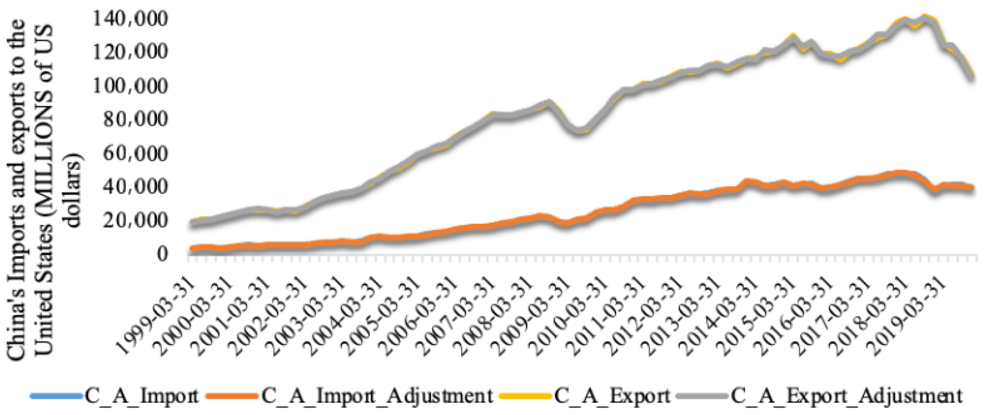
3.1. History of China–US Trade

To demonstrate the dynamic trade relationship between China and the US, we express the quarterly trade volume of China’s imports and exports to the United States as ${\alpha }^{(0)}(\kappa )$ and ${\beta }^{(0)}(\kappa )$, respectively, and the cumulative series of imports and exports as ${\alpha }^{(1)}(\kappa )$ and ${\beta }^{(1)}(\kappa )$, which can be obtained by an accumulation based on the first quarter of 1999. From 1999 to 2019, China’s trade exports to the United States were far greater than imports, and the trade surplus showed an expanding trend. Since China joined the World Trade Organization (WTO) in 2001, China’s export trade volume has shown a substantial growth trend. In 2008, the US financial crisis swept the world, which had significant effects on China–US trade. This was reflected in the significant reduction in the scale of China’s export trade to the US and the slight decrease in import trade volume in the third quarter of 2008. Thereafter, the import and export volume showed an upward trend. In 2014, the world experienced a period of economic recovery, and overall world demand declined. China’s export volume to the United States dropped again, and then imports and exports showed an uptrend. Until the outbreak of the China–US trade war in 2018, China’s export trade volume to the US decreased significantly; in contrast, the import volume decreased slightly. In summary, three evident processes drove the decline in the scale of China–US trade, mainly affected by the financial crisis [43] and sluggish world market demand. In the past 20 years, what has the dynamic relationship been between China and the US and what kind of evolutionary processes are the key research questions posed here? Since quarterly data are susceptible to seasonal factors, we first use the X12-seasonal adjustment method to adjust the original data seasonally. As shown in Figure 2, the influences of seasonal factors are minor, and there is little difference between the adjusted quarterly and actual series.

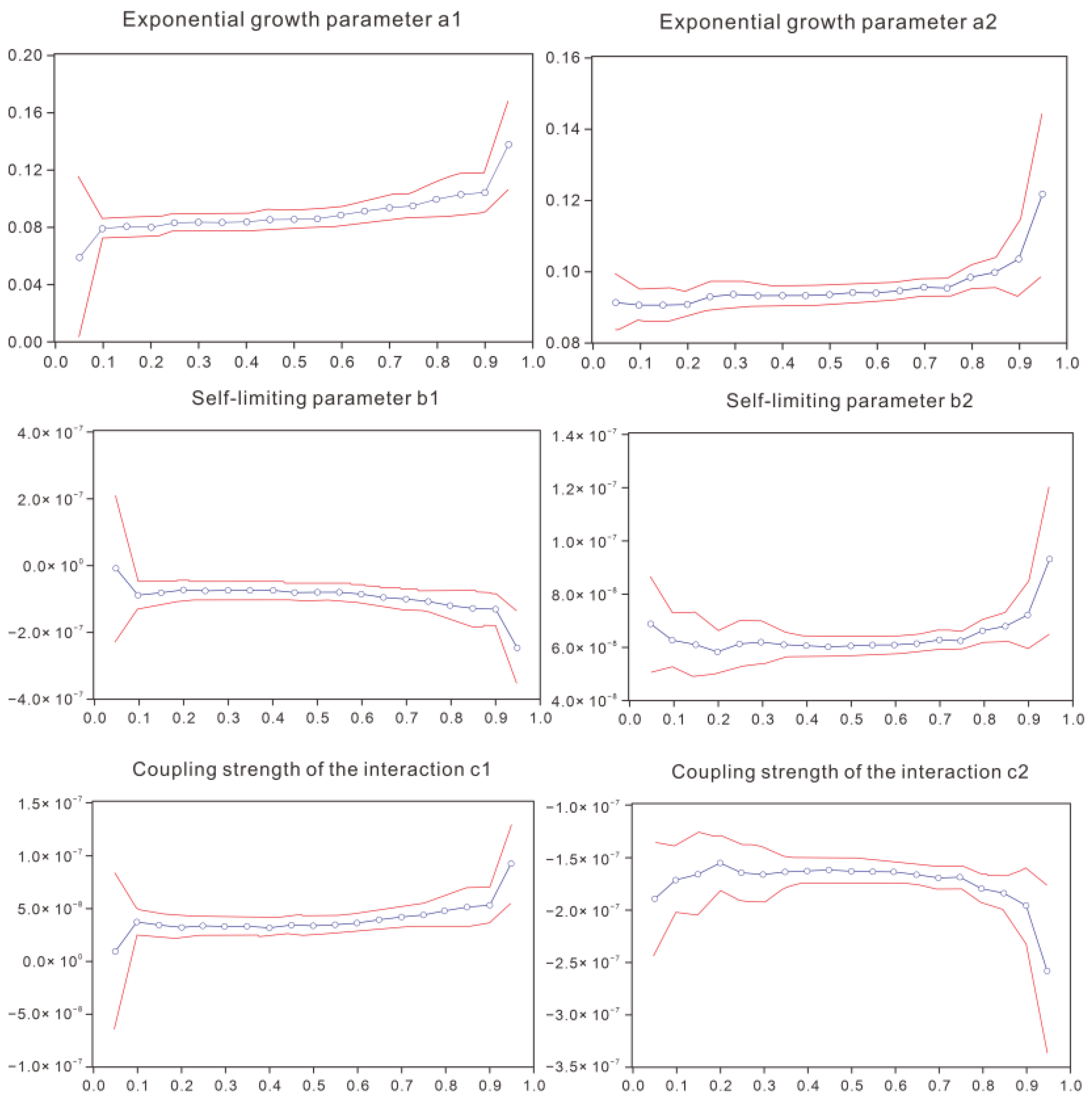
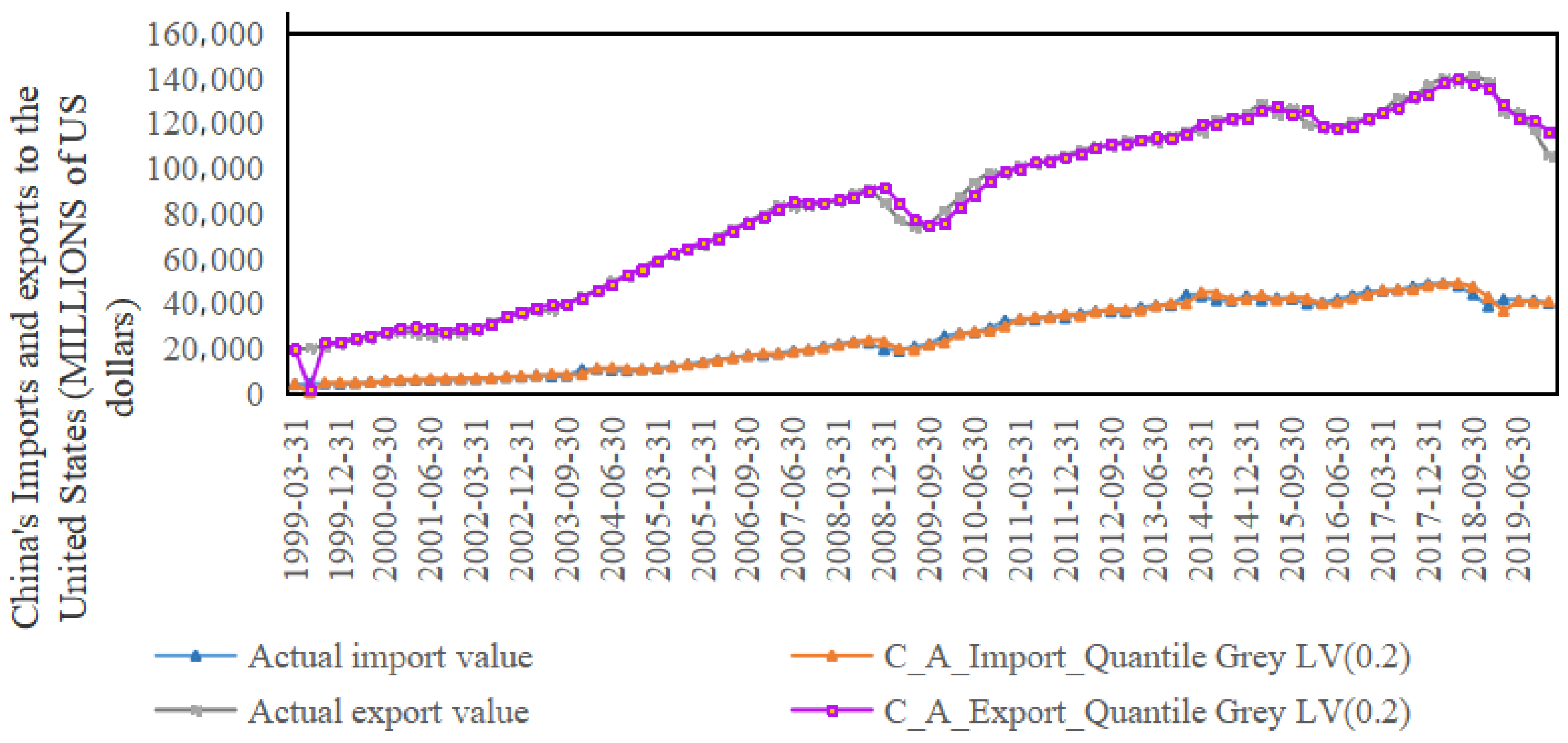
3.2. Simulation Using the QGLV Model

In the parameter estimation of the QGLV model, the improved simplex method in quantile regression is used to estimate each parameter. The parameters of the QGLV model at each quantile are shown in Figure 3, the red line shows the upper and lower limits of the 95% confidence interval of each quantile, and the blue line part represents coefficient estimates of the quantile regression model. Under different quantile values, the results of each parameter are different, while the traditional OLS regression only reflects the average, which embodies the advantages of quantile regression estimation to a certain extent. Especially when quantile ${\tau }_1,{\tau }_2\in (0,1)$ is close to the two extremes of the range are the parameters quite different. With the exception of variables ${\left({\phi }_{\alpha }^{(1)}(\kappa )\right)}^2$ and ${\phi }_{\alpha }^{(1)}(\kappa ){\phi }_{\beta }^{(1)}(\kappa )$ failing the significance test when estimating the parameter $b_{{\tau }_2}$ and $c_{{\tau }_2}$ at 0.05 quantile, the optimal QGLV model did not consider the 0.05 quantile, and all other quantile variables passed statistical test criteria (p < 0.05).

Based on parameter estimation at each quantile, the MAPE results of the QGLV model constructed herein are listed in

Table 2. MAPE of the QGLV model.

Quantile	China’s Imports from the US (%)	China’s Exports to the US (%)	Quantile	China’s Imports from the US (%)	China’s Exports to the US (%)
0.05	5.045	3.689	0.55	5.273	3.706
0.10	5.262	3.660	0.60	5.294	3.709
0.15	5.254	3.664	0.65	5.333	3.718
0.20	5.236	3.680	0.70	5.364	3.725
0.25	5.253	3.699	0.75	5.385	3.724
0.30	5.251	3.700	0.80	5.453	3.755
0.35	5.254	3.696	0.85	5.503	3.770
0.40	5.247	3.698	0.90	5.524	3.813
0.45	5.271	3.697	0.95	6.226	4.080
0.50	5.268	3.705

. The MAPEs of the QGLV model of China’s imports to the United States are all less than 6.3%, and the fitting error is minimised at the 0.05 quantile at 5.045%; the MAPE of the QGLV model of China’s exports to the United States at each quantile is all less than 4.1%. In addition, after passing the test, the error of the QGLV model at the 0.2 quantiles is minimised, with an average error of 4.458%. The model has an excellent fitting effect and strong robustness, making it suitable for analysing the dynamic trade relationship between China and the US.

On the premise that the minimum MAPE fitted by the two equations is the goal and the test is passed, we obtain the model parameter estimation results based on the optimal quantile (

Table 3. Continuous estimation of the QGLV model at the optimal quantile.

China’s Import Trade Volume to the US				China’s Exports to the US
Parameter	Value	t	p	Parameter	Value	t	p
${\widehat{a}}_1$	$7.93\times {10}^{-2}$	23.72	0.00	${\widehat{a}}_2$	$9.06\times {10}^{-2}$	47.86	0.00
${\widehat{b}}_1$	$-7.59\times {10}^{-8}$	−4.65	0.00	${\widehat{b}}_2$	$5.79\times {10}^{-8}$	14.07	0.00
${\widehat{c}}_1$	$3.16\times {10}^{-8}$	5.93	0.00	${\widehat{c}}_2$	$-1.56\times {10}^{-7}$	−11.83	0.00

).

If the t-test is passed at the 5% confidence interval then the estimated values of $\widehat{a}$ are all valid.

Natural growth coefficients ${\widehat{a}}_1$ (>0) and ${\widehat{a}}_2$ (>0) show that the natural growth rates of import and export scale indicators are positive when they are unaffected by external interference. This parameter can realise the further expansion of the import and export scale without relying on other policy support or conflict; however, from the perspective of the degree of promotion, the growth momentum of China’s imports to the US is less than that driving the development of China’s exports to the US.

The restrictive parameters ${\widehat{b}}_1$ (<0) and ${\widehat{b}}_2$ (>0) denote that there is a marginal increasing effect in the growth process of imports and a marginal decreasing effect in the growth process of exports, and the range of the increasing effect of imports is greater than the one of the decreasing effects of exports. This shows that the development potential of China’s imports to the US is greater than that of China’s exports to the US.

From an interaction point of view, ${\widehat{c}}_1$ (>0) and ${\widehat{c}}_2$ (<0) imply that there is a predator–prey relationship, which is not conducive to China’s imports to the US but is conducive to China’s export to the United States. There are two possible mechanisms driving this relationship:

(1)

Comparison of export competitiveness. China’s imports of products and services from the United States meet the needs of the domestic population and partly replace the demand for domestic products and services, resulting in transporting domestic products and services abroad and promoting the development of China’s foreign trade. For the greater demand in the United States, China provides products at lower prices and complete services. Compared with the products exported by the United States to China, China’s exports to the US are more competitive, which has a considerable effect on the domestic market of the United States. For instance, after China acceded to the WTO, the significant reduction in export tariffs made its products and services competitive, and its global market share increased. The increased competitiveness of Chinese exports has affected the imports and exports of domestic companies in the United States. In addition, Athukorala and Yamashita [44] also believed that the China–US trade imbalance was a structural phenomenon caused by China’s critical role in the global production network as a final product assembly centre. Therefore, China’s imports to the US have become a driving mechanism to promote China’s exports to the US, and China’s export competitiveness to the US is more vital than that of the US to China.

(2)

Financial environment in the US. After financial liberalisation, the US financial supervision was relaxed, bank reserve ratios decreased, and loans increased. At the same time, the real estate and stock markets boomed, and the wealth effect stimulated household consumption and reduced the incentive to save. The US trade surplus equals the difference between US consumption and savings. To a certain extent, this change promotes imports from the US to China and restrains the trend of US trade exports to China, which changes the global economy. After the financial crisis, the international market as a whole was depressed. There was an inevitable interdependence between the two sides during the economic recovery. The China–US trade relationship evolved from a competitive relationship to a symbiotic and predator–prey relationship.

According to the correspondence between parameters of continuity and the discrete model, the parameter conversion results are listed in

Table 4. QGLV model discrete estimation of optimal dissociation points.

Parameter	Estimated Value	Parameter	Estimated Value
${\widehat{\lambda }}_1$	1.08 × 100	${\widehat{\lambda }}_2$	6.06 × 10−8
${\widehat{\theta }}_1$	1.09 × 100	${\widehat{\theta }}_2$	3.29 × 10−8
${\widehat{\gamma }}_1$	−7.90 × 10−8	${\widehat{\gamma }}_2$	−1.63 × 10−7

. In addition, continuous and discrete parameter estimation results of each quantile are shown in Appendix A.

The prediction results of the optimal QGLV model are as shown in Equations (30) and (31):

$${\widehat{\alpha }}_{(0.2)}(\kappa +1)=\frac{1.08\alpha (\kappa )}{1+1.09\alpha (\kappa )-7.90\times {10}^{-8}\beta (\kappa )}, \kappa =1,2,\dots ,n$$

(30)

$${\widehat{\beta }}_{(0.2)}(\kappa +1)=\frac{6.06\times {10}^{-8}\beta (\kappa )}{1+3.29\times {10}^{-8}\beta (\kappa )-1.63\times {10}^{-7}\alpha (\kappa )}, \kappa =1,2,\dots ,n$$

(31)

According to Equations (11) and (12), the predicted values of import and export can be obtained by calculation. As shown in Figure 4, the predicted values of import and export are close to actual values, and the fitting effect is good.

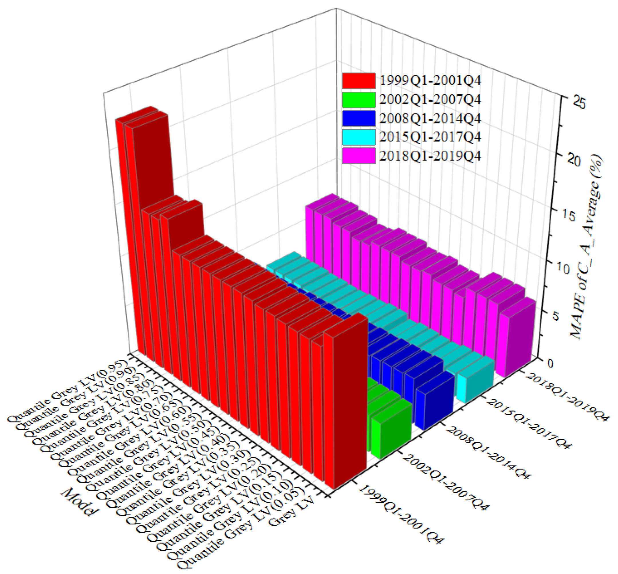
3.3. Comparison of the GLV and QGLV Models

For the quarterly data on the scale of China’s import and export trade to the United States, we construct the GLV and the QGLV models, from which actual and predicted values are shown in Figure 5. We estimate the QGLV model under 19 equally spaced quantiles, respectively. The average MAPE is less than 5.2%, and the prediction is accurate. The error of the QGLV model’s optimal quantile is lower than that of the GLV model, which means that the QGLV model achieved the purpose of reducing the error. The QGLV model can significantly improve the LV model’s accuracy, which plays an optimisation role for data with outliers. The results of the QGLV model are more robust.

3.4. Equilibrium Analysis

Not all equilibrium points are meant for discussion in China–US bilateral trade relations. For example, point B has a negative number, which we do not include in the discussion. At the same time, in a fluctuating environment, not all equilibrium points are stable. The equilibrium points and stable points of the relationship between China’s imports and exports to the United States are analysed by consideration of the eigenvalue method of the Jacobian matrix. When the matrix is negative definite, the equilibrium point is stable; otherwise, it is unstable. The calculated results are displayed in

Table 5. Equilibrium point and stability analysis of the QGLV model based on the optimal quantile (0.2).

Equilibrium	Eigenvalue	Equilibrium Value	Stability
$O\left(0,0\right)$	$\left(0.0793,0.0906\right)$	$O\left(0,0\right)$	Unstable
$E\left(0,\frac{a_2}{b_2}\right)$	$\left(-0.0906,0.0299\right)$	$E\left(0,1.56\times {10}^6\right)$	Unstable
$N\left(\frac{a_1}{b_1},0\right)$	$\left(-0.0793,-0.0725\right)$	$N\left(-1.05\times {10}^6,0\right)$	Unstable
$M\left(\frac{a_1{b}_2-a_2{c}_{12}}{b_1{b}_2-c_{12}{c}_{21}},\frac{a_2{b}_1-a_1{c}_{21}}{b_1{b}_2-c_{21}{c}_{12}}\right)$	$\left(-0.0619,-0.2880\right)$	$M\left(3.24\times {10}^6,1.03\times {10}^7\right)$	Stable

; the eigenvalue and the equilibrium values are both scalars.

(1)

Explanation of ecosystem analysis. In ecosystem analysis, there are four possible outcomes of the rivalry. As shown in Table 5, trade in both countries has been suppressed at the first equilibrium point $O\left(0,0\right)$. Trade in one country wins, while trade in another country is suppressed at the second point $E\left(0,1.56\times {10}^6\right)$ and the third point $N\left(-1.05\times {10}^6,0\right)$. The import–export relationship will stabilise at the fourth equilibrium point $M\left(3.24\times {10}^6,1.03\times {10}^7\right)$, indicating that the cumulative volume of China’s imports to the United States will stabilise at million dollars, and the cumulative volume of China’s exports to the United States will stabilise at USD $1.03\times {10}^7$ million dollars.

(2)

Explanation of economic model. Comparative advantage theory: China has a comparative advantage in labour-intensive products and can produce goods in large quantities at low cost. In contrast, the United States has a comparative advantage in technology-intensive and capital-intensive products. Via the trade cooperation between the two countries, the optimal allocation of resources and the improvement in efficiency can be achieved to achieve mutual benefit and win–win results. Absolute advantage theory: In China–US trade, China has the advantages of abundant labour and relatively low cost, while the United States has absolute advantages in high-tech fields and innovative industries. Because of their respective advantages, China has become the world’s factory, and the United States has become a leader in technology and innovation. However, when trade imbalance and bias gradually emerge, adjusting trade policies and balancing interests between the two sides will lead to trade friction.

3.5. Phased China–US Trade Relations Based on the QGLV Model

China–US trade relations exhibited a predator–prey relationship across all 19 quantiles during the sample period. Then, we perform a phased analysis of China–US trade relations based on the characteristics of the quarterly data on China–US trade. The quarterly data on China–US trade from 1999 to 2019 are divided into five stages: Phase 1 is from 1999 to 2001, Phase 2 is from 2002 to 2007, Phase 3 is from 2008 to 2014, Phase 4 is from 2015 to 2017, and Phase 5 is from 2018 to 2019. The segmentation events of these phases were China’s entry into the WTO (2001), the outbreak of the financial crisis (2008), the period of global economic recovery (2015), and the outbreak of the China–US trade war (2018). We establish the QGLV model for these five stages. The MAPE results are illustrated in Figure 6, which are the fitting errors of China’s imports and exports volume to the United States and the average fitting error of imports and exports volume, respectively. With the exception of the MPAE in the first phase under parameter estimation at the two quantiles of 0.95 and 0.9 exceeding 20%, the MAPEs at the remaining quantiles are all less than 20%, ranging from 12.00% to 17.26%; the MAPEs of the other four periods are all less than 10%, which shows that the model fitting effect is good, and shows strong robustness, suitable for further dynamic relationship analysis. Based on the estimation of each parameter, the quality and accuracy of the fit in each period are shown in Figure 7, which has high consistency and coincidence with the original data.

According to the positive and negative signs of $c_1$ and $c_2$, we ascertain whether the dynamic trade relationship between China and the US is a predator–prey relationship, a competitive relationship, or a symbiotic relationship, and its evolution. As shown in Figure 8, because the fitting errors of quantiles 0.90 and 0.95 are large, the estimations at these two quantiles are not considered.

We took 19 quantiles at intervals of 0.05 and estimated the parameters $c_1$ and $c_2$ at each quantile. Due to the selection of different quantiles, the error weights in the objective function are different, resulting in differences in estimated parameters. According to Figure 8(1), in all quantiles, which indicates that the China–US bilateral trade relationship is a predator–prey relationship. In these quantiles, China’s imports from the US are the predator, and China’s exports to the US are the prey. This relationship is conducive to China’s imports from the US but not conducive to China’s exports to the United States. This may be due to China’s high export tariffs before joining the WTO, which led to the lack of core competitiveness of Chinese products and services, thus inhibiting China’s export trade. According to Figure 8(2), $c_1>0$ in most quantiles, China and the United States compete most of the time. In a few quantiles, $c_1>0$ and $c_2<0$, China’s imports from the US are the predator, and China’ exports to the US are the prey. This indicates that the relationship at this stage is not stable enough, remaining mainly competitive, and may also present a predator–prey relationship. After China entered the WTO, its global market share increased, which has a certain influence on international trade, including the United States. According to Figure 8(3), $c_1$ are both unstable, and in most, $c_2<0$, which indicates that since the third stage, the China–US trade relationship may evolve from a competition-oriented model in the second stage to a predator–predator relationship and even a symbiosis and predator–predator relationship. This period of time changed from China’s exports to the US being a predator to China’s imports from the US being a predator. After the financial crisis, with the overall international market depression, the two sides had a certain mutual interdependence. According to Figure 8(4), in most quantiles $c_2<0$, the China–US trade relationship once again presents a significant predator–prey relationship. China’s imports from the US are the predators, and China’s exports to the US are the prey. According to Figure 8(5), most quantiles (16/19) $c_1>0$ indicate that China–US trade relations are gradually showing a more competitive relationship. This shows that China–US trade war frictions are frequent, leading to obvious competition in the bilateral market between China and the US, and bilateral trade is inhibited under this relationship. In conclusion, in the past 20 years, from 1999 to 2019, the China–US trade relationship has evolved from a significant predator–prey relationship to an unobvious competitive relationship, returned to a predator–prey relationship, and finally evolved into a more significant competitive relationship.

4. Conclusions and Policy Implications

In the present work, quantile regression technology is introduced into the Lotka–Volterra ecosystem analysis framework and a QGLV model is constructed to identify the dynamic trade relationship between China and the United States. The study found that the fitting of the QGLV model can achieve high accuracy; the MAPE of the optimal QGLV model reaches 5.236% and 3.680%, and the model shows strong robustness. From 1999 to 2019, the long-term trade relationship between China and the US presented a significant predator–prey relationship because China’s exports to the United States inhibited China’s imports from the United States. This is similar to the view of Athens and Yamashita [44] that the trade imbalance between China and the United States is a structural phenomenon caused by China’s critical role in the global production network. Further, to identify the details of this relationship, we divide the import and export trade volumes into five stages and reveal the phased dynamic relationship underpinning China–US trade. The relationship undergoes an inevitable evolution wherein it changes from a significant predator–prey relationship to an unobvious competitive relationship, back to the predator–prey relationship, and finally, a more significant competitive relationship.

In the case of limited data and information, the proposed model can be an essential reference tool for future research on international trade relations. This research will help national decision makers make correct judgments in the rapidly changing international market and make appropriate decisions to maintain the advantage of sustainable development.

With the development of a new scientific and technological revolution, China–US trade relations have entered a new era. The China–US trade relationship has its nature and particularity in different products and services in the network era. Therefore, our future work will focus on applying the QGLV model to identify China–US trade competition in different fields in the digital economy.

According to the conclusion, we propose two policy implications:

(1)

The leading tone of China–US trade policy should be cooperation, not competition. Some trade frictions between China and the United States are sometimes not a collision of substantive interests but a misunderstanding caused by a lack of mutual understanding. China–US trade relations are mutually beneficial, with opportunities outstripping challenges and cooperation outstripping competition. Trade frictions can be effectively managed. With the development of China’s economy, the scale of China–US trade has been expanding, bringing tangible benefits to the economic development of the two countries and the lives of the two peoples. As major global trading countries, China and the United States have a profound basis for complementation. Bilateral trade is mutually beneficial and win–win, with massive potential for development and broad prospects. As a developed economy, the United States has long been a global leader in manufacturing and rich in high-tech resources. China has transformed from a traditional industrial structure to a modern industry as an emerging economy. The complementation of trade between significant countries is essential for China–US strategic trade cooperation. Amid the tortuous recovery of the global economy and trade, the two countries actively promote and shape the process of scientific and technological cooperation at the international level, which can further tap the potential of complementary trade structures, expand market cooperation space, and jointly improve the welfare of the people of the two countries and the world.

(2)

Promoting trade balance between China and the United States manifests high-quality foreign trade development. For a country’s foreign trade, export and import are like two sides of a coin, and any policies and measures that ignore one aspect will bring about the consequences of economic imbalance. It is found in this paper that China’s export to the United States inhibits China’s imports from the United States. China should have a deep and comprehensive understanding of the United States in many aspects such as politics, economy, society and culture. It should actively expand imports, promote trade balance, reduce trade surplus with the United States, promote the development of global multilateral trade, reduce trade friction, and promote international trade balance. The United States can appropriately liberalise export controls, reduce high tariffs, and promote trade balance. China and the United States need to take a step back and think before taking a step forward. The sustained and balanced development of China–US trade is necessary for the long-term economic and trade cooperation between the two countries.

References

1. Jiang, Z.; Yoon, S. Dynamic co-movement between oil and stock markets in oil-importing and oil-exporting countries: Two types of wavelet analysis. Energy Econ. 2020, 90, 104835. [Google Scholar] [CrossRef]
2. Mahmood, H.; Alkhateeb, T.; Furqan, M. Exports, imports, Foreign Direct Investment and CO2 emissions in North Africa: Spatial analysis. Energy Rep. 2020, 6, 2403–2409. [Google Scholar] [CrossRef]
3. Lotka, A. The law of evolution as a maximal principle. Hum. Biol. 1945, 17, 167–194. [Google Scholar]
4. Volterra, E. On the dynamic stress-strain relationship for plastic and elastic materials. In Proceedings of the 6th International Congress for Applied Mechanics, Paris, France, 22–29 September 1946. [Google Scholar]
5. Rouvinen, P. Diffusion of Digital Mobile Telephony: Are Developing Countries Different? Telecommun. Policy 2006, 30, 46–63. [Google Scholar] [CrossRef]
6. Ma, Z.S. Chaotic populations in genetic algorithms. Appl. Soft Comput. 2012, 12, 2409–2424. [Google Scholar] [CrossRef]
7. Tseng, F.M.; Yu, J.R. A two stage fuzzy piecewise logistic model for penetration forecasting. Appl. Soft Comput. 2014, 21, 149–158. [Google Scholar] [CrossRef]
8. Hong, J.; Koo, H.; Kim, T. Easy, reliable method for mid-term demand forecasting based on the Bass model: A hybrid approach of NLS and OLS. Eur. J. Oper. Res. 2016, 248, 681–690. [Google Scholar] [CrossRef]
9. Kreng, V.; Wang, T.; Wang, H.T. Tripartite dynamic competition and equilibrium analysis on global television market. Comput. Ind. Eng. 2012, 63, 75–81. [Google Scholar] [CrossRef]
10. Michalakelis, C.; Christodoulos, C.; Varoutas, D.; Sphicopoulos, T. Dynamic estimation of markets exhibiting a prey–predator behavior. Expert Syst. Appl. 2012, 39, 7690–7700. [Google Scholar] [CrossRef]
11. Wang, Y.S.; Wu, H. Global dynamics of Lotka-Volterra equations characterizing multiple predators competing for one prey. J. Math. Anal. Appl. 2020, 491, 124293. [Google Scholar] [CrossRef]
12. Mao, S.H.; Zhu, M.; Wang, X.P.; Xiao, X.P. Grey-Lotka-Volterra model for the competition and cooperation between third-party online payment systems and online banking in China. Appl. Soft Comput. 2020, 95, 106501. [Google Scholar] [CrossRef]
13. Guo, D.; Yan, W.; Gao, X.; Hao, Y.; Xu, Y.; Wenjuan, E.; Tan, X.; Zhang, T. Forecast of passenger car market structure and environmental impact analysis in China. Sci. Total Environ. 2021, 772, 144950. [Google Scholar] [CrossRef]
14. Grabner, C.; Hahn, H.; Leopold-Wildburger, U.; Pickl, S. Analyzing the sustainability of harvesting behavior and the relationship to personality traits in a simulated Lotka-Volterra biotope. Eur. J. Oper. Res. 2009, 193, 761–767. [Google Scholar] [CrossRef]
15. Neokosmidis, I.; Avaritsiotis, N.; Ventoura, Z. Modeling gender evolution and gap in science and technology using ecological dynamics. Expert Syst. Appl. 2013, 40, 3481–3490. [Google Scholar] [CrossRef]
16. Modis, T. US Nobel laureates: Logistic growth versus Volterra–Lotka. Technol. Forecast. Soc. Chang. 2011, 78, 559–564. [Google Scholar] [CrossRef]
17. Chiang, S. An application of Lotka–Volterra model to Taiwan’s transition from 200 mm to 300 mm silicon wafers. Technol. Forecast. Soc. Chang. 2012, 79, 383–392. [Google Scholar] [CrossRef]
18. Hung, H.C.; Tsai, Y.S.; Wu, M.C. A modified Lotka–Volterra model for competition forecasting in Taiwan’s retail industry. Comput. Ind. Eng. 2014, 77, 70–79. [Google Scholar] [CrossRef]
19. Agrrawal, P.; Clark, J.M.; Agarwal, R.; Kale, J.K. An inter-temporal study of etf liquidity and underlying factor transition (2009–2014). J. Trading 2014, 9, 69–78. [Google Scholar] [CrossRef]
20. Ditzen, J. Cross-country convergence in a general Lotka-Volterra model. Spat. Econ. Anal. 2018, 13, 191–211. [Google Scholar] [CrossRef]
21. Marasco, A.; Picucci, A.; Romano, A. Market share dynamics using Lotka–Volterra models. Technol. Forecast. Soc. Chang. 2016, 105, 49–62. [Google Scholar] [CrossRef]
22. Li, X.; Shen, H.L.; Feng, Y.G. Study on the parameter grey estimation of logistic and Lotka-Volterra model. Coll. Math. 2004, 20, 82–87. [Google Scholar]
23. Deng, J.L. The Basis of Grey Theory; Huazhong University of Science & Technology Press: Wuhan, China, 2002. [Google Scholar]
24. Wu, L.F.; Liu, S.F.; Wang, Y.N. Grey Lotka–Volterra model and its application. Technol. Forecast. Soc. Chang. 2012, 79, 1720–1730. [Google Scholar] [CrossRef]
25. Gatabazi, P.; Mba, J.C.; Pindza, E.; Labuschagne, C. Grey Lotka–Volterra models with application to cryptocurrencies adoption. Chaos Solitons Fractals 2019, 122, 47–57. [Google Scholar] [CrossRef]
26. Hung, H.; Chiu, Y.; Huang, H. An enhanced application of Lotka–Volterra model to forecast the sales of two competing retail formats. Comput. Ind. Eng. 2017, 109, 325–334. [Google Scholar] [CrossRef]
27. Zhang, S.; Meng, X.Z.; Feng, T.; Zhang, T.H. Dynamics analysis and numerical simulations of a stochastic non-autonomous predator–prey system with impulsive effects. Nonlinear Anal. Hybrid Syst. 2017, 26, 19–37. [Google Scholar] [CrossRef]
28. Amore, P.; Fernández, F.M. On the application of the Lindstedt-Poincaré method to the Lotka-Volterra system. Ann. Phys. 2018, 396, 293–303. [Google Scholar] [CrossRef]
29. Shi, L.L.; Chen, Y.Q. Existence and Iterative Algorithms of Solutions for Lotka-Volterra Competition Model. IAENG Int. J. Appl. Math. 2023, 53, 1–6. [Google Scholar]
30. Zhao, K.; Yu, S.J.; Wu, L.F.; Wu, X.; Wang, L. Carbon emissions prediction considering environment protection investment of 30 provinces in China. Environ. Res. 2024, 224, 117914. [Google Scholar] [CrossRef]
31. Morris, S.; Pratt, D. Analysis of the Lotka-Volterra competition equations as a technological substitution model. Technol. Forecast. Soc. Chang. 2003, 70, 103–133. [Google Scholar] [CrossRef]
32. Lazzús, J.A.; Vega-Jorquera, P.; López-Caraballo, C.H.; Palma-Chilla, L.; Salfate, I. Parameter estimation of a generalized Lotka–Volterra system using a modified PSO algorithm. Appl. Soft Comput. 2020, 96, 106606. [Google Scholar] [CrossRef]
33. Zhou, J.; Fang, R.; Li, Y.; Zhang, B. Parameter optimization of nonlinear grey Bernoulli model using particle swarm optimization. Appl. Math. Comput. 2009, 207, 292–299. [Google Scholar] [CrossRef]
34. Agrrawal, P. An automation algorithm for harvesting capital market information from the web. Manag. Financ. 2009, 35, 427–438. [Google Scholar]
35. Wang, C.; Hsu, L. Using genetic algorithms grey theory to forecast high technology industrial output. Appl. Math. Comput. 2008, 195, 256–263. [Google Scholar] [CrossRef]
36. Wu, L.F.; Wang, Y.N. Estimation the parameters of Lotka-Volterra model based on grey direct modelling method and its application. Expert Syst. Appl. 2011, 38, 6412–6416. [Google Scholar] [CrossRef]
37. Wang, Z.X.; Jv, Y.Q. A novel grey prediction model based on quantile regression. Commun. Nonlinear Sci. Numer. Simul. 2021, 95, 105617. [Google Scholar] [CrossRef]
38. Marinakis, Y.D.; White, R.; Walsh, S.T. Lotka–Volterra signals in ASEAN currency exchange rates. Phys. A Stat. Mech. Its Appl. 2020, 545, 123743. [Google Scholar] [CrossRef]
39. Leslie, P. A Stochastic Model for Studying the Properties of Certain Biological Systems by Numerical Methods. Biometrika 1958, 45, 16–31. [Google Scholar] [CrossRef]
40. Koenker, R.; Bassett, J. Regression Quantiles. Econometrica 1978, 46, 33–50. [Google Scholar] [CrossRef]
41. Barrodale, I.; Roberts, F.D.K. An improved algorithm for discrete L1 linear approximation. SIAM J. Numer. Anal. 1973, 10, 839–848. [Google Scholar] [CrossRef]
42. Pei, L.L.; Wang, Z.X.; Ye, D.J. Estimation of the Competitive Relationships between Amazon, Alibaba, and Suning Based on a Grey Tripartite Lotka-Volterra Model. J. Grey Syst. 2017, 29, 30–48. [Google Scholar]
43. Agrrawal, P.; Skaves, M. Seasonality in stock and bond etfs (2001–2014): The months are getting mixed up but santa delivers on time. Soc. Sci. Electron. Publ. 2015, 24, 129–143. [Google Scholar] [CrossRef]
44. Athukorala, P.; Yamashita, N. Global Production Sharing and China–US Trade Relations. China World Econ. 2009, 17, 39–56. [Google Scholar] [CrossRef]
Figure 1. Modelling process of the quantile grey Lotka–Volterra model.
Fractalfract 08 00171 g001
Figure 2. China–US quarterly trade volume before and after seasonal adjustment from 1999 to 2019.
Fractalfract 08 00171 g002
Figure 3. Parameter estimation of each quantile under 95% confidence intervals.
Fractalfract 08 00171 g003
Figure 4. Results of optimal model fitting for quarterly data of China–US trade volume from 1999 to 2019.
Fractalfract 08 00171 g004
Figure 5. Comparison of errors between the QGLV model and GLV model.
Fractalfract 08 00171 g005
Figure 6. MAPE of the QGLV model at each quantile in each period.
Fractalfract 08 00171 g006aFractalfract 08 00171 g006b
Figure 7. Forecast of China–US trade at the optimal quantiles in each period.
Fractalfract 08 00171 g007aFractalfract 08 00171 g007b
Figure 8. Values of c 1 and c 2 in each time.
Fractalfract 08 00171 g008