


Dynamic Fractional-Order Grey Prediction Model with GWO and MLP for Forecasting Overseas Talent Mobility in China


Abstract
1. Introduction
1.1. Background
1.2. Overseas Talent Mobility Prediction
1.3. Grey Models
1.3.1. Basic Principles of Grey Forecasting Models
1.3.2. Advancements in Fractional-Order Grey Prediction Models
1.4. Contributions
2. Methodology
2.1. FGM(1,1)
2.2. GWO
2.3. MLP
2.4. Proposed MGDFGM(1,1)
2.5. Model Evaluation Criteria
3. Empirical Results
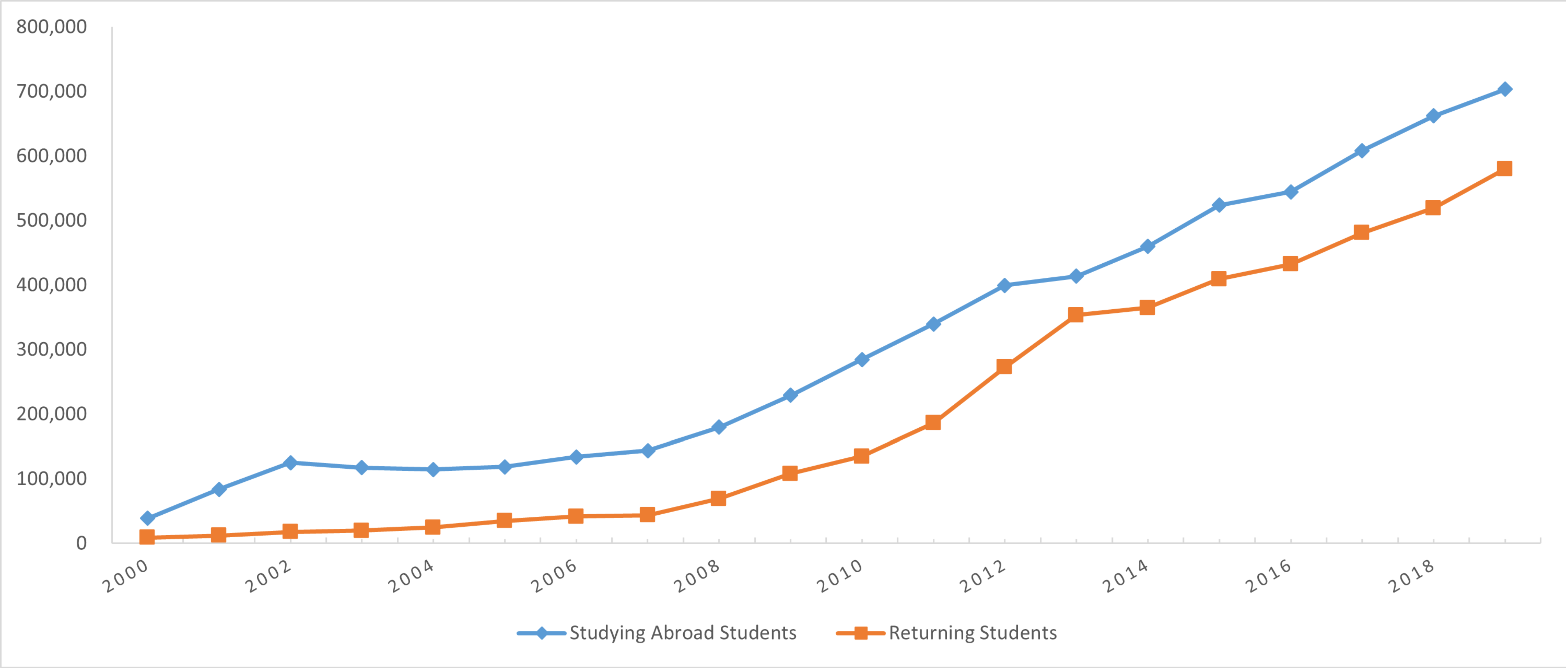
3.1. Data Description
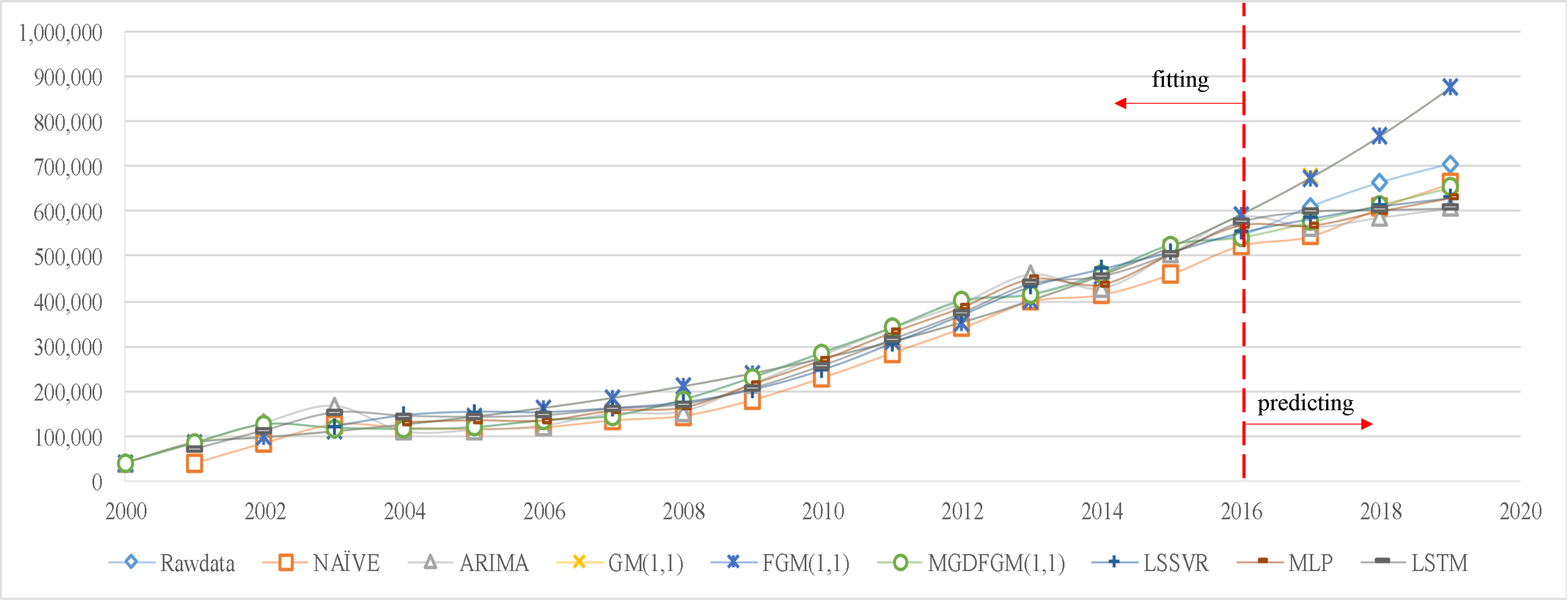
3.2. Experiment 1: Students Studying Abroad
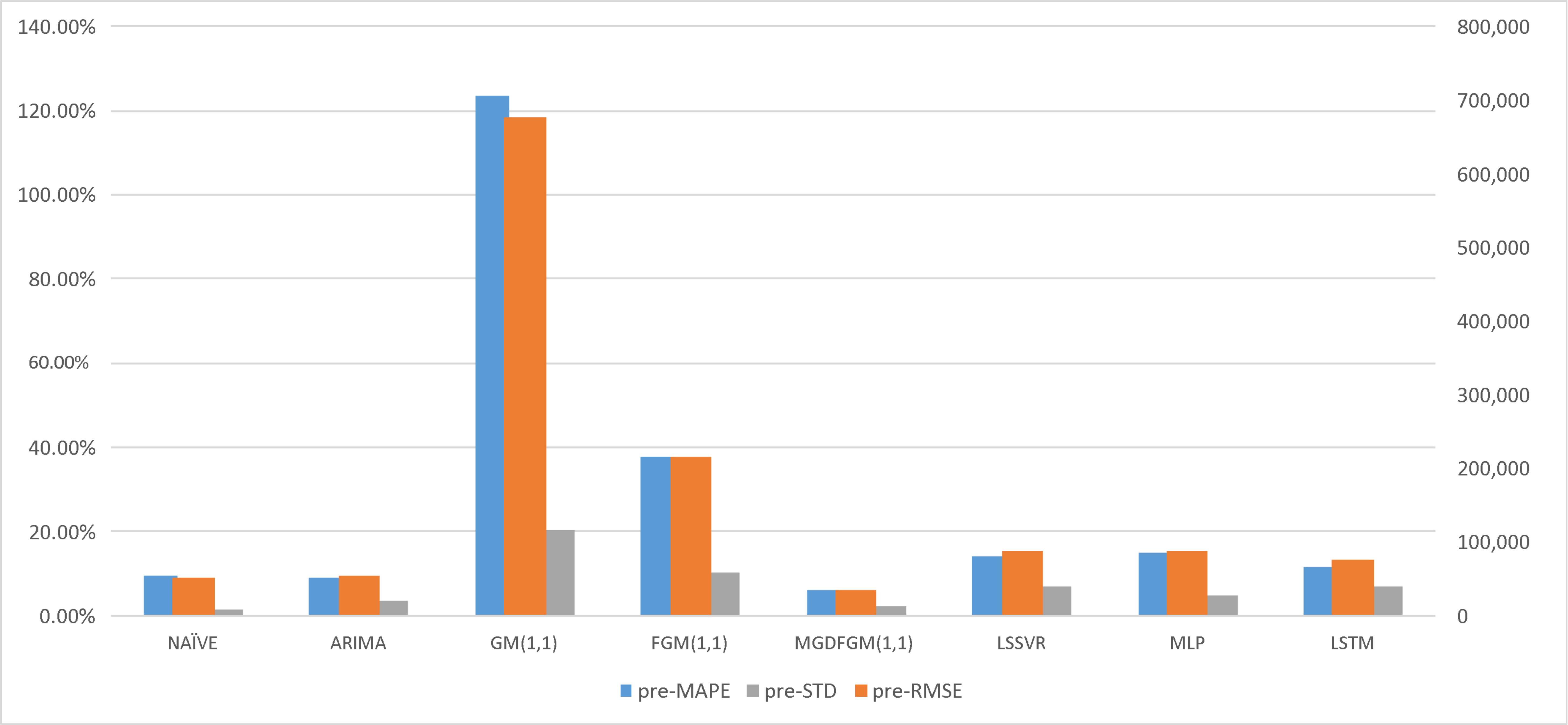
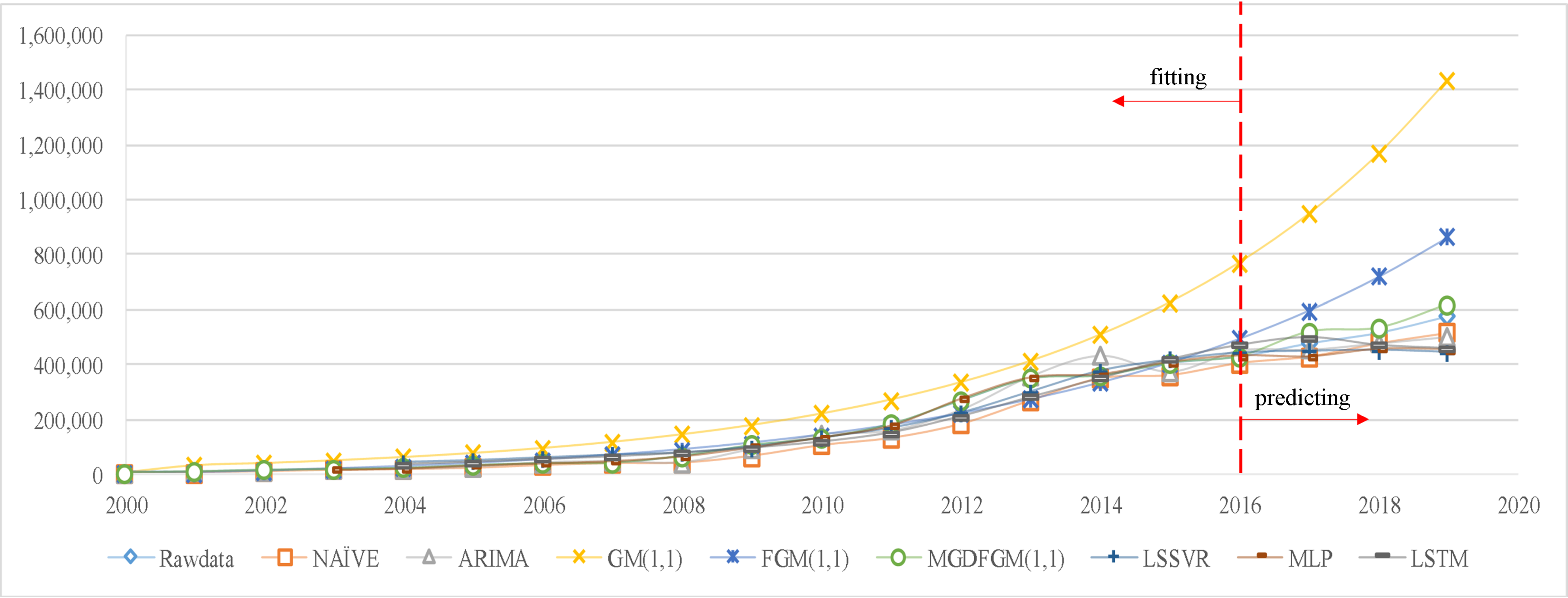
3.3. Experiment 2: Returned Overseas Students
4. Discussion
5. Conclusions
Author Contributions
Funding
Data Availability Statement
Conflicts of Interest
References
- Lin, D.; Zheng, W.; Lu, J.; Liu, X.; Wright, M. Forgotten or Not? Home Country Embeddedness and Returnee Entrepreneurship. J. World Bus. 2019, 54, 1–13. [Google Scholar] [CrossRef]
- Xiong, W.; Mok, K.H. Critical Reflections on Mainland China and Taiwan Overseas Returnees’ Job Searches and Career Development Experiences in the Rising Trend of Anti-Globalisation. High. Educ. Policy 2020, 33, 413–436. [Google Scholar] [CrossRef]
- Dai, O.; Liu, X. Returnee Entrepreneurs and Firm Performance in Chinese High-Technology Industries. Int. Bus. Rev. 2009, 18, 373–386. [Google Scholar] [CrossRef]
- Li, W.; Sadowski-Smith, C.; Yu, W. Return Migration and Transnationalism: Evidence from Highly Skilled Academic Migration. Pap. Appl. Geogr. 2018, 4, 243–255. [Google Scholar] [CrossRef]
- Zhang, C.; Guan, J. Returnee Policies in China: Does a Strategy of Alleviating the Financing Difficulty of Returnee Firms Promote Innovation? Technol. Forecast. Soc. Chang. 2021, 164, 120509. [Google Scholar] [CrossRef]
- Xu, H.; Yu, Z.; Yang, J.; Xiong, H.; Zhu, H. Dynamic Talent Flow Analysis with Deep Sequence Prediction Modeling. IEEE Trans. Knowl. Data Eng. 2019, 31, 1926–1939. [Google Scholar] [CrossRef]
- Fernandes, J. Trends in International Student Mobility: A Study of the Relationship between the UK and China and the Chinese Student Experience in the UK. Scott. Educ. Rev. 2006, 38, 133–144. [Google Scholar] [CrossRef]
- Iannelli, C.; Huang, J. Trends in Participation and Attainment of Chinese Students in UK Higher Education. Stud. High. Educ. 2014, 39, 805–822. [Google Scholar] [CrossRef]
- Knight, J. Student Mobility and Internationalization: Trends and Tribulations. Res. Comp. Int. Educ. 2012, 7, 20–33. [Google Scholar] [CrossRef]
- Lin, S.; Liu, J. Has Excess Epidemic Prevention Changed Chinese Students’ Willingness to Study Abroad: Three Rounds of the Same Volume Survey Based on the New “Push–Pull” Theory. Humanit. Soc. Sci. Commun. 2023, 10, 662. [Google Scholar] [CrossRef]
- Mok, K.H.; Xiong, W.; Ke, G.; Cheung, J.O.W. Impact of COVID-19 Pandemic on International Higher Education and Student Mobility: Student Perspectives from Mainland China and Hong Kong. Int. J. Educ. Res. 2021, 105, 101718. [Google Scholar] [CrossRef] [PubMed]
- Yang, M. What Attracts Mainland Chinese Students to Australian Higher Education. Innov. Dev. 2007, 4, 1–12. [Google Scholar]
- Ozturgut, O. Best Practices in Recruiting and Retaining International Students in the U.S. Curr. Issues Educ. 2013, 16. [Google Scholar]
- Ke, P.; Wu, G. Study on Prediction of the Number of Study Abroad Based on GM (1.1) Model. Value Eng. 2012, 31, 318–319. [Google Scholar] [CrossRef]
- Li, Q. The Development of China’s Study Abroad Education and It’s Countermeasures. J. Syst. Sci. Inf. 2010, 8, 87–96. [Google Scholar]
- Ren, Y.; Jiang, P. Forecasting the Number of Students Studying Abroad and Returned Students Studying Abroad Based on Grey Forecasting Model. J. Manag. Decis. Sci. 2020, 3, 41–53. [Google Scholar] [CrossRef]
- Jiang, P.; Wu, G.; Hu, Y.-C.; Zhang, X.; Ren, Y. Novel Fractional Grey Prediction Model with the Change-Point Detection for Overseas Talent Mobility Prediction. Axioms 2022, 11, 432. [Google Scholar] [CrossRef]
- Feng, Z.; Yu, D. Prediction of abroad Chinese students and its impact on household consumption. J. Nanjing Univ. Inf. Sci. Technol. 2014, 6, 369–373. [Google Scholar] [CrossRef]
- Totska, O. Modeling the migration of ukrainians to study abroad. Sci. J. Pol. Univ. 2018, 28, 11–16. [Google Scholar] [CrossRef]
- Yang, C.; Duan, X. Prediction of the number of students studying abroad in China: Based on the time series prediction method. Sci. Technol. Economy Mark. 2016, 1, 119–121. [Google Scholar]
- Yang, S.; Chen, H.-C.; Chen, W.-C.; Yang, C.-H. Forecasting Outbound Student Mobility: A Machine Learning Approach. PLoS ONE 2020, 15, e0238129. [Google Scholar] [CrossRef] [PubMed]
- Bijak, J.; Disney, G.; Findlay, A.M.; Forster, J.J.; Smith, P.W.F.; Wiśniowski, A. Assessing Time Series Models for Forecasting International Migration: Lessons from the United Kingdom. J. Forecast. 2019, 38, 470–487. [Google Scholar] [CrossRef]
- Li, Z. Forecast and Analysis of Reasons for Changes in the Number of Students Studying Abroad. Highlights Sci. Eng. Technol. 2022, 24, 107–118. [Google Scholar] [CrossRef]
- Hu, Z. Research on Combination Forecasting of the Number of Students Studying Abroad Based on L1 Norm. J. Chongqing Technol. Bus. Univ. Nat. Sci. Ed. 2022, 39, 61–69. [Google Scholar] [CrossRef]
- Wei, Y. Prediction of international students and returnees based on grey neural network model. Bus. Econ. 2010, 4, 4–6+122. [Google Scholar]
- Hu, Y.-C.; Wu, G.; Jiang, P. Tourism Demand Forecasting Using Nonadditive Forecast Combinations. J. Hosp. Tour. Res. 2023, 47, 775–799. [Google Scholar] [CrossRef]
- Xie, N.; Wang, R. A Historic Review of Grey Forecasting Models. J. Grey Syst. 2017, 29, 1. [Google Scholar]
- Wei, B.; Xie, N. Parameter Estimation for Grey System Models: A Nonlinear Least Squares Perspective. Commun. Nonlinear Sci. 2021, 95, 105653. [Google Scholar] [CrossRef]
- Xiangmei, M.; Leping, T.; Chen, Y.; Lifeng, W. Forecast of Annual Water Consumption in 31 Regions of China Considering GDP and Population. Sustain. Prod. Consum. 2021, 27, 713–736. [Google Scholar] [CrossRef]
- Zhao, X.; Ma, X.; Cai, Y.; Yuan, H.; Deng, Y. Application of a Novel Hybrid Accumulation Grey Model to Forecast Total Energy Consumption of Southwest Provinces in China. Grey Syst. Theory Appl. 2023, 13, 629–656. [Google Scholar] [CrossRef]
- Mao, Q.; Xiao, X.; Gao, M.; Wang, X.; He, Q. Nonlinear Fractional Order Grey Model of Urban Traffic Flow Short-Term Prediction. J. Grey Syst. 2018, 30, 1–17. [Google Scholar]
- Guo, X.; Li, J.; Liu, S.; Xie, N.; Yang, Y.; Zhang, H. Analyzing the Aging Population and Density Estimation of Nanjing by Using a Novel Grey Self-Memory Prediction Model Under Fractional-Order Accumulation. J. Grey Syst. 2022, 34, 34–52. [Google Scholar]
- Li, X.; Zhao, Z.; Zhao, Y.; Zhou, S.; Zhang, Y. Prediction of Energy-Related Carbon Emission Intensity in China, America, India, Russia, and Japan Using a Novel Self-Adaptive Grey Generalized Verhulst Model. J. Clean. Prod. 2023, 423, 138656. [Google Scholar] [CrossRef]
- Wu, L.; Liu, S.; Yao, L.; Yan, S.; Liu, D. Grey System Model with the Fractional Order Accumulation. Commun. Nonlinear Sci. 2013, 18, 1775–1785. [Google Scholar] [CrossRef]
- Wu, L.; Gao, X.; Xiao, Y.; Yang, Y.; Chen, X. Using a Novel Multi-Variable Grey Model to Forecast the Electricity Consumption of Shandong Province in China. Energy 2018, 157, 327–335. [Google Scholar] [CrossRef]
- Hu, Y.-C. Forecast Combination Using Grey Prediction with Fuzzy Integral and Time-Varying Weighting in Tourism. Grey Syst. Theory Appl. 2023, 13, 808–827. [Google Scholar] [CrossRef]
- Yang, Y.; Xiong, J.; Zhao, L.; Wang, X.; Hua, L.; Wu, L. A Novel Method of Blockchain Cryptocurrency Price Prediction Using Fractional Grey Model. Fractal Fract. 2023, 7, 547. [Google Scholar] [CrossRef]
- Gao, M.; Yang, H.; Xiao, Q.; Goh, M. A Novel Fractional Grey Riccati Model for Carbon Emission Prediction. J. Clean. Prod. 2021, 282, 124471. [Google Scholar] [CrossRef]
- Ma, X.; Xie, M.; Wu, W.; Zeng, B.; Wang, Y.; Wu, X. The Novel Fractional Discrete Multivariate Grey System Model and Its Applications. Appl. Math. Model. 2019, 70, 402–424. [Google Scholar] [CrossRef]
- Pu, B.; Nan, F.; Zhu, N.; Yuan, Y.; Xie, W. UFNGBM (1,1): A Novel Unbiased Fractional Grey Bernoulli Model with Whale Optimization Algorithm and Its Application to Electricity Consumption Forecasting in China. Energy Rep. 2021, 7, 7405–7423. [Google Scholar] [CrossRef]
- Yan, C.; Wu, L.; Liu, L.; Zhang, K. Fractional Hausdorff Grey Model and Its Properties. Chaos Solitons Fractals 2020, 138, 109915. [Google Scholar] [CrossRef]
- Lifeng, W.U.; Sifeng, L.; Ligen, Y. Grey Model with Caputo Fractional Order Derivative. Syst. Eng. Theory Pract. 2015, 35, 1311–1316. [Google Scholar]
- Ma, X.; Wu, W.; Zeng, B.; Wang, Y.; Wu, X.; Wang, Y.; Wang, L.; Ye, L.; Ma, X.; Wu, W.; et al. A Novel Self-Adaptive Fractional Multivariable Grey Model and Its Application in Forecasting Energy Production and Conversion of China. Eng. Appl. Artif. InteL 2022, 115, 105319. [Google Scholar] [CrossRef]
- Wu, W.-Z.; Pang, H.; Zheng, C.; Xie, W.; Liu, C. Predictive Analysis of Quarterly Electricity Consumption via a Novel Seasonal Fractional Nonhomogeneous Discrete Grey Model: A Case of Hubei in China. Energy 2021, 229, 120714. [Google Scholar] [CrossRef]
- Zhicun, X.; Meng, D.; Lifeng, W. Evaluating the Effect of Sample Length on Forecasting Validity of FGM(1,1). Alex. Eng. J. 2020, 59, 4687–4698. [Google Scholar] [CrossRef]
- Hu, Y.-C. Forecasting Tourism Demand Using Fractional Grey Prediction Models with Fourier Series. Ann. Oper. Res. 2021, 300, 467–491. [Google Scholar] [CrossRef]
- Lao, T.; Chen, X.; Zhu, J. The Optimized Multivariate Grey Prediction Model Based on Dynamic Background Value and Its Application. Complexity 2021, 2021, 6663773. [Google Scholar] [CrossRef]
- Zeng, B.; Tan, Y.; Xu, H.; Quan, J.; Wang, L.; Zhou, X. Forecasting the Electricity Consumption of Commercial Sector in Hong Kong Using a Novel Grey Dynamic Prediction Model. J. Grey Syst. 2018, 30, 157–172. [Google Scholar]
- Faris, H.; Aljarah, I.; Al-Betar, M.A.; Mirjalili, S. Grey Wolf Optimizer: A Review of Recent Variants and Applications. Neural Comput. Appl. 2018, 30, 413–435. [Google Scholar] [CrossRef]
- Xie, W.; Wu, W.-Z.; Liu, C.; Zhang, T.; Dong, Z. Forecasting Fuel Combustion-Related CO2 Emissions by a Novel Continuous Fractional Nonlinear Grey Bernoulli Model with Grey Wolf Optimizer. Environ. Sci. Pollut. Res. 2021, 28, 38128–38144. [Google Scholar] [CrossRef]
- Gan, K.; Sun, S.; Wang, S.; Wei, Y. A Secondary-Decomposition-Ensemble Learning Paradigm for Forecasting PM2.5 Concentration. Atmos. Pollut. Res. 2018, 9, 989–999. [Google Scholar] [CrossRef]
- Mirjalili, S.; Mirjalili, S.M.; Lewis, A. Grey Wolf Optimizer. Adv. Eng. Softw. 2014, 69, 46–61. [Google Scholar] [CrossRef]
- Dehghani, M.; Riahi-Madvar, H.; Hooshyaripor, F.; Mosavi, A.; Shamshirband, S.; Zavadskas, E.; Chau, K. Prediction of Hydropower Generation Using Grey Wolf Optimization Adaptive Neuro-Fuzzy Inference System. Energies 2019, 12, 289. [Google Scholar] [CrossRef]
- Iliyasu, A.M.; Fouladinia, F.; Salama, A.S.; Roshani, G.H.; Hirota, K. Intelligent Measurement of Void Fractions in Homogeneous Regime of Two Phase Flows Independent of the Liquid Phase Density Changes. Fractal Fract. 2023, 7, 179. [Google Scholar] [CrossRef]
- Xing, G.; Sun, S.; Bi, D.; Guo, J.; Wang, S. Seasonal and Trend Forecasting of Tourist Arrivals: An Adaptive Multiscale Ensemble Learning Approach. J. Tour. Res. 2022, 24, 425–442. [Google Scholar] [CrossRef]
- Xie, G.; Wang, S.; Zhao, Y.; Lai, K.K. Hybrid Approaches Based on LSSVR Model for Container Throughput Forecasting: A Comparative Study. Appl. Soft Comput. 2013, 13, 2232–2241. [Google Scholar] [CrossRef]
- Koo, E.; Kim, G. Centralized Decomposition Approach in LSTM for Bitcoin Price Prediction. Expert. Syst. Appl. 2024, 237, 121401. [Google Scholar] [CrossRef]
- Yang, C.-H.; Chang, P.-Y. Forecasting the Demand for Container Throughput Using a Mixed-Precision Neural Architecture Based on CNN–LSTM. Mathematics 2020, 8, 1784. [Google Scholar] [CrossRef]
- Hyndman, R.J.; Athanasopoulos, G. Forecasting: Principles and Practice, 3rd ed.; OTexts: Melbourne, Australia, 2021. [Google Scholar]
- Lewis, C.D. Industrial and Business Forecasting Methods; Butterworth Scientific: London, UK, 1982. [Google Scholar]


| MAPE | Prediction Accuracy |
|---|---|
| <10% | High |
| 10%~20% | Good |
| 20%~50% | Reasonable |
| ≥50% | Inaccurate |
| Year | Raw Data | NAÏVE | ARIMA | GM(1,1) | FGM(1,1)0.996 * | MGDFGM(1,1) | LSSVR | MLP | LSTM |
|---|---|---|---|---|---|---|---|---|---|
| 2000 | 38,989 | 38,972 | 38,989 | 38,989 | 38,989 | ||||
| 2001 | 83,973 | 38,989 | 83,925 | 84,348 | 83,973 | 83,967 | 71,366.6 | ||
| 2002 | 125,179 | 83,973 | 128,957 | 96,053 | 95,786 | 125,021 | 112,968 | ||
| 2003 | 117,307 | 125,179 | 166,385 | 109,382 | 109,181 | 117,267 | 121,492 | 152,380 | |
| 2004 | 114,682 | 117,307 | 109,435 | 124,561 | 124,407 | 114,509 | 146,178 | 131,131 | 144,757 |
| 2005 | 118,515 | 114,682 | 112,057 | 141,846 | 141,727 | 117,996 | 154,107 | 135,170 | 142,203 |
| 2006 | 134,000 | 118,515 | 122,348 | 161,530 | 161,437 | 133,996 | 152,883 | 134,678 | 145,932 |
| 2007 | 144,000 | 134,000 | 149,485 | 183,945 | 183,871 | 143,846 | 162,169 | 156,904 | 160,957 |
| 2008 | 179,800 | 144,000 | 154,000 | 209,471 | 209,408 | 179,573 | 174,756 | 163,657 | 170,785 |
| 2009 | 229,300 | 179,800 | 215,600 | 238,538 | 238,477 | 229,223 | 203,112 | 216,073 | 206,504 |
| 2010 | 284,700 | 229,300 | 278,800 | 271,640 | 271,570 | 284,403 | 247,008 | 269,823 | 257,169 |
| 2011 | 339,700 | 284,700 | 340,100 | 309,335 | 309,245 | 340,434 | 306,115 | 330,792 | 315,399 |
| 2012 | 399,600 | 339,700 | 394,700 | 352,261 | 352,135 | 399,299 | 369,108 | 386,585 | 374,476 |
| 2013 | 413,900 | 399,600 | 459,500 | 401,143 | 400,964 | 413,979 | 432,742 | 449,600 | 439,746 |
| 2014 | 459,800 | 413,900 | 428,200 | 456,809 | 456,553 | 460,217 | 471,384 | 437,233 | 455,448 |
| 2015 | 523,700 | 459,800 | 505,700 | 520,200 | 519,840 | 524,651 | 509,673 | 505,371 | 506,007 |
| 2016 | 544,500 | 523,700 | 587,600 | 592,387 | 591,889 | 541,626 | 552,778 | 569,180 | 576,499 |
| 2017 | 608,400 | 544,500 | 565,300 | 674,591 | 673,915 | 576,005 | 583,651 | 568,450 | 599,465 |
| 2018 | 662,100 | 608,400 | 586,100 | 768,203 | 767,298 | 614,180 | 610,998 | 600,414 | 603,235 |
| 2019 | 703,500 | 662,100 | 606,900 | 874,805 | 873,611 | 652,201 | 629,872 | 629,747 | 607,004 |
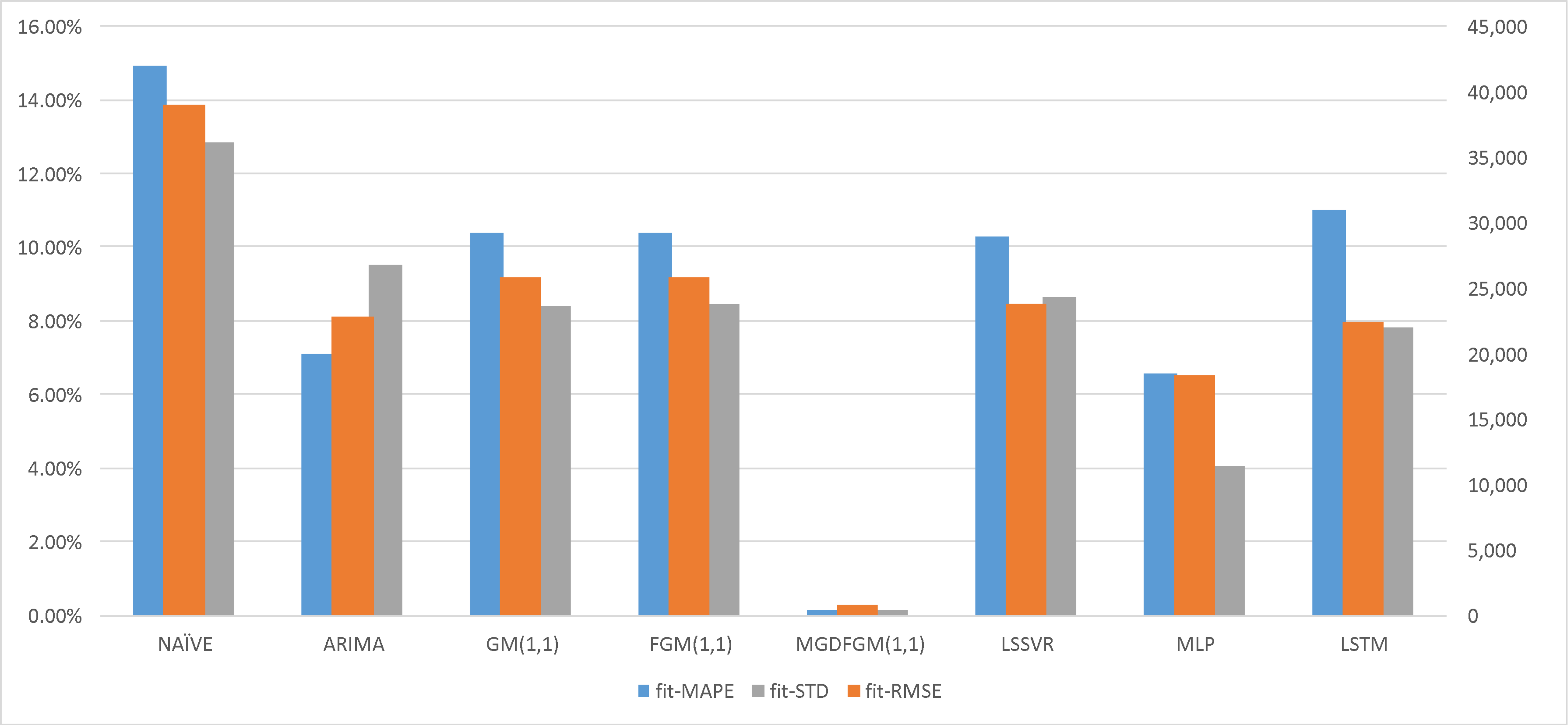
| fit-MAPE | 14.926% | 7.086% | 10.385% | 10.365% | 0.140% | 10.288% | 6.560% | 11.004% | |
| fit-RMSE | 39,040.076 | 22,790.422 | 25,839.728 | 25,809.518 | 808.903 | 23,765.415 | 18,291.157 | 22,414.081 | |
| fit-STD | 12.831% | 9.509% | 8.414% | 8.435% | 0.144% | 8.665% | 4.060% | 7.811% | |
| pre-MAPE | 8.166% | 10.765% | 17.085% | 16.946% | 6.618% | 7.417% | 8.789% | 8.025% | |
| pre-RMSE | 53,792.379 | 75,200.111 | 122,453.680 | 121,513.661 | 44,636.843 | 53,681.188 | 60,112.866 | 65,463.477 | |
| pre-STD | 1.886% | 2.760% | 5.550% | 5.526% | 0.915% | 2.621% | 1.642% | 5.038% | |
| Year | Raw Data | NAÏVE | ARIMA | GM(1,1) | FGM(1,1)0.068 * | MGDFGM(1,1) | LSSVR | MLP | LSTM |
|---|---|---|---|---|---|---|---|---|---|
| 2000 | 9121 | 9117 | 9121 | 9121 | 9121 | ||||
| 2001 | 12,243 | 9121 | 12,248 | 34,537 | 6789 | 12,241 | |||
| 2002 | 17,945 | 12,243 | 15,365 | 42,486 | 12,794 | 17,970 | |||
| 2003 | 20,152 | 17,945 | 23,647 | 52,263 | 20,152 | 20,132 | 19,127 | ||
| 2004 | 24,726 | 20,152 | 22,359 | 64,291 | 29,216 | 24,722 | 44,202 | 24,340 | 37,403 |
| 2005 | 34,987 | 24,726 | 29,300 | 79,087 | 40,354 | 35,090 | 50,551 | 35,501 | 45,467 |
| 2006 | 42,000 | 34,987 | 45,248 | 97,288 | 53,991 | 42,024 | 60,850 | 42,709 | 55,631 |
| 2007 | 44,000 | 42,000 | 49,013 | 119,678 | 70,622 | 44,011 | 70,737 | 51,589 | 65,230 |
| 2008 | 69,300 | 44,000 | 46,000 | 147,221 | 90,830 | 69,448 | 79,232 | 68,560 | 78,745 |
| 2009 | 108,300 | 69,300 | 94,600 | 181,102 | 115,304 | 108,317 | 100,032 | 101,068 | 97,266 |
| 2010 | 134,800 | 108,300 | 147,300 | 222,781 | 144,852 | 134,715 | 133,752 | 136,911 | 119,511 |
| 2011 | 186,200 | 134,800 | 161,300 | 274,052 | 180,425 | 185,155 | 169,655 | 180,479 | 153,151 |
| 2012 | 272,900 | 186,200 | 237,600 | 337,123 | 223,145 | 271,950 | 224,884 | 277,007 | 212,751 |
| 2013 | 353,500 | 272,900 | 359,600 | 414,708 | 274,327 | 350,066 | 302,361 | 353,513 | 282,737 |
| 2014 | 364,800 | 353,500 | 434,100 | 510,149 | 335,519 | 360,460 | 378,376 | 364,754 | 351,406 |
| 2015 | 409,100 | 364,800 | 376,100 | 627,554 | 408,538 | 407,814 | 418,206 | 409,247 | 420,185 |
| 2016 | 432,500 | 409,100 | 453,400 | 771,979 | 495,512 | 431,939 | 444,275 | 432,387 | 472,462 |
| 2017 | 480,900 | 432,500 | 455,900 | 949,642 | 598,942 | 520,592 | 450,457 | 428,860 | 500,388 |
| 2018 | 519,400 | 480,900 | 479,300 | 1,168,190 | 721,753 | 535,106 | 454,004 | 456,216 | 471,904 |
| 2019 | 580,300 | 519,400 | 502,700 | 1,437,040 | 867,375 | 621,056 | 446,190 | 455,069 | 460,205 |
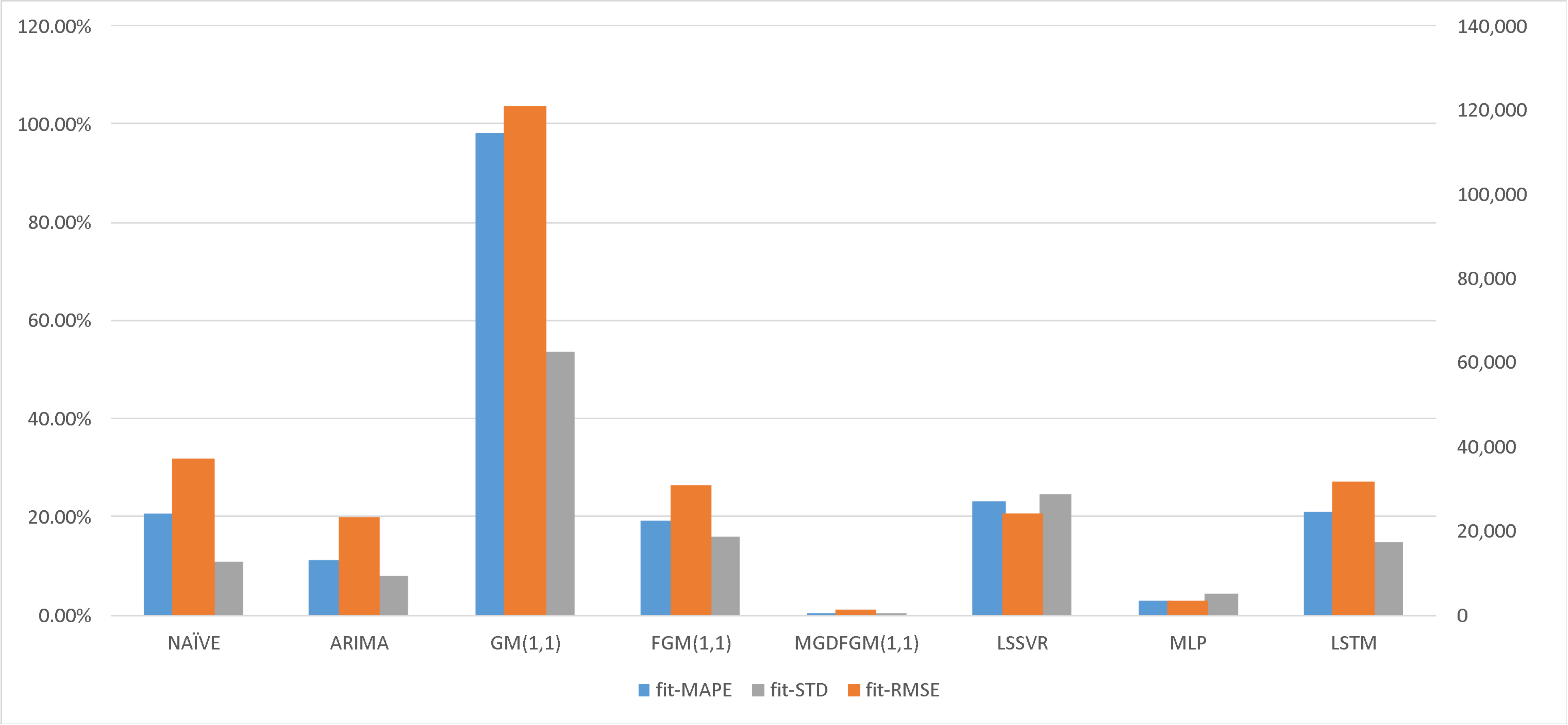
| fit-MAPE | 20.69% | 11.31% | 98.29% | 19.20% | 0.28% | 23.17% | 2.93% | 20.96% | |
| fit-RMSE | 37,402.22 | 23,277.02 | 120,732.29 | 30,798.67 | 1471.37 | 23,955.40 | 3448.65 | 31,584.52 | |
| fit-STD | 10.89% | 7.87% | 53.73% | 16.07% | 0.34% | 24.49% | 4.40% | 14.99% | |
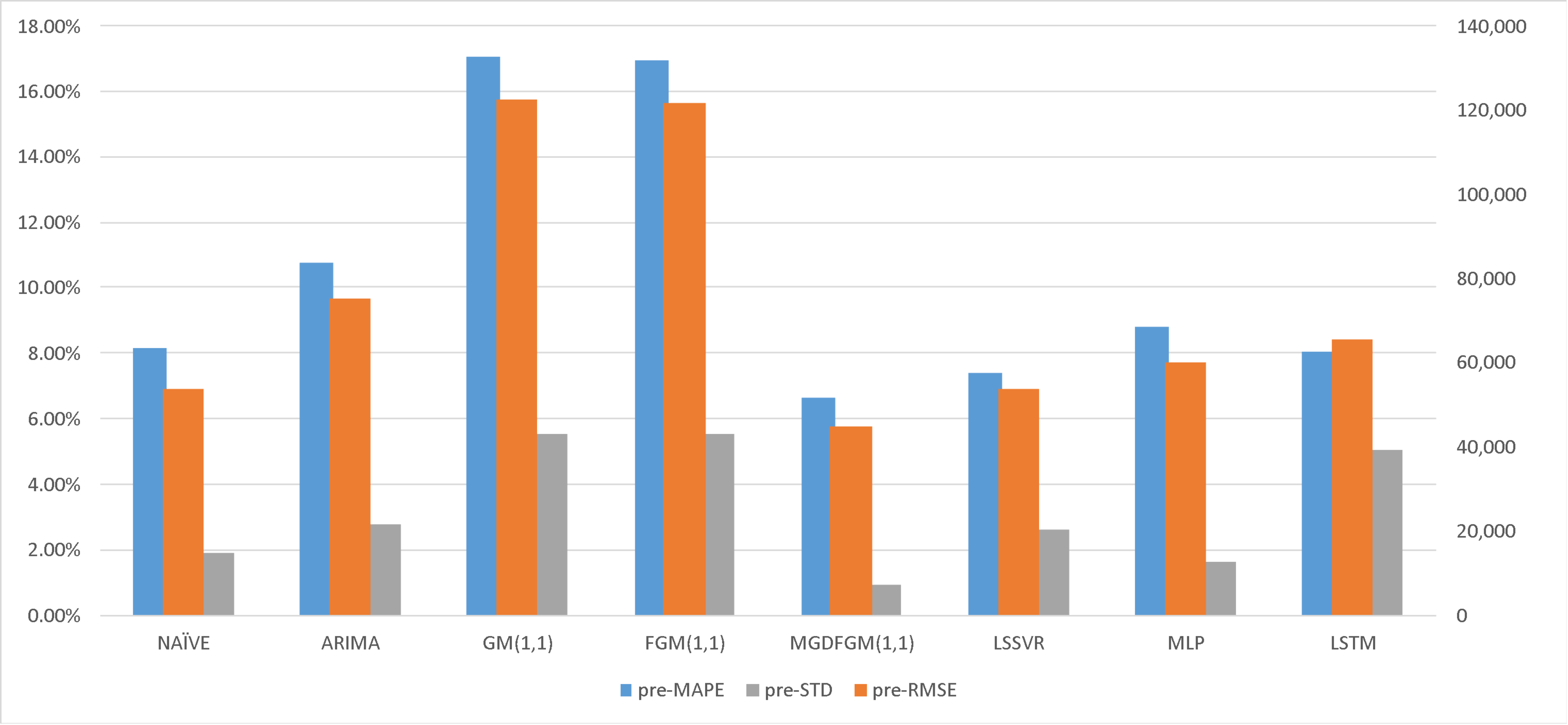
| pre-MAPE | 9.32% | 8.76% | 123.34% | 37.66% | 6.10% | 14.01% | 14.86% | 11.30% | |
| pre-RMSE | 50,111.94 | 52,455.60 | 676,917.27 | 213,925.81 | 34,074.24 | 87,918.34 | 86,377.43 | 75,406.59 | |
| pre-STD | 1.36% | 3.42% | 20.51% | 10.22% | 2.23% | 6.92% | 4.79% | 6.96% | |
Disclaimer/Publisher’s Note: The statements, opinions and data contained in all publications are solely those of the individual author(s) and contributor(s) and not of MDPI and/or the editor(s). MDPI and/or the editor(s) disclaim responsibility for any injury to people or property resulting from any ideas, methods, instructions or products referred to in the content. |
© 2024 by the authors. Licensee MDPI, Basel, Switzerland. This article is an open access article distributed under the terms and conditions of the Creative Commons Attribution (CC BY) license (https://creativecommons.org/licenses/by/4.0/).
Share and Cite
Wu, G.; Fu, H.; Jiang, P.; Chi, R.; Cai, R. Dynamic Fractional-Order Grey Prediction Model with GWO and MLP for Forecasting Overseas Talent Mobility in China. Fractal Fract. 2024, 8, 217. https://doi.org/10.3390/fractalfract8040217
Wu G, Fu H, Jiang P, Chi R, Cai R. Dynamic Fractional-Order Grey Prediction Model with GWO and MLP for Forecasting Overseas Talent Mobility in China. Fractal and Fractional. 2024; 8(4):217. https://doi.org/10.3390/fractalfract8040217
Chicago/Turabian StyleWu, Geng, Haiwei Fu, Peng Jiang, Rui Chi, and Rongjiang Cai. 2024. "Dynamic Fractional-Order Grey Prediction Model with GWO and MLP for Forecasting Overseas Talent Mobility in China" Fractal and Fractional 8, no. 4: 217. https://doi.org/10.3390/fractalfract8040217
APA StyleWu, G., Fu, H., Jiang, P., Chi, R., & Cai, R. (2024). Dynamic Fractional-Order Grey Prediction Model with GWO and MLP for Forecasting Overseas Talent Mobility in China. Fractal and Fractional, 8(4), 217. https://doi.org/10.3390/fractalfract8040217