Abstract
The aim of this research is to define a design approach for implementing composite materials in a component of an industrial vehicle, having weight reduction as the primary goal. Through the schematisation of the problem and analytical analysis, the definition of a new geometry, a material and production process, and numerical simulations and experimental studies to test the new solution, an optimization process of the chosen geometry is proposed. After the definition of the process, an applicative example is presented, analysing a front underrun protection device in two different solutions: one made of glass-fibre-reinforced polymer and the other of carbon-fibre-reinforced polymer. An economic comparison has also been conducted between the new configurations and the traditional steel version, showing a weight reduction of approximately 55% for the carbon-fibre-reinforced polymer solution and around 18% for the glass-fibre-reinforced polymer solution. These weight reductions are achievable through a reinvestment that can be amortized in less than five years, thanks to fuel consumption savings.
1. Introduction
The mechanical design process is an essential component of engineering that entails a methodical approach to developing efficient and effective solutions for many applications. As technology advances, the tools currently accessible in the market substantially contribute to the reduction in costs and time spent on research. To ensure their reliability and identify potential issues, it is essential to validate these virtual models through physical testing. Mechanical testing yields critical data that validate simulation accuracy and allow designers to enhance their models, resulting in more resilient and efficient outputs. As a result of the advancements in design and testing methodologies in the last decades, innovative materials have emerged as viable alternatives to traditional ones. Nowadays, the adoption of fibre-reinforced polymer (FRP) composite structures instead of traditional metallic components in structural design offers several advantages, including reduced fuel or oil consumption, emission reductions, and improved performance, due to their lower mass and the low energy costs involved in their production process [1]. In the literature, the study of lightweight machine parts has been applied not only to transport vehicles but also to earth-moving machinery [2,3], hoist equipment [4,5], automotive applications [6,7], and even aviation [8,9,10].
The optimization process for lightweight components has already been extensively studied in the literature. Saeedi et al. [11] defined general procedures for designing and analyzing fibre-reinforced polymer parts for railroad vehicles, particularly for car bodies, bogies, wheelsets, and other structural components such as rail sleepers. Dragatogiannis et al. [12] analysed a deck reinforcement on a composite yacht for crane installation, proposing a methodology flowchart for the structural analysis. Rahman et al. [13], while studying ship structures made from composite materials, presented a process to evaluate the engineering properties of multidirectional laminates. Gardie et al. [14] investigated the use of composite materials in car wheels, highlighting their advantages compared to aluminium. Ciampaglia et al. [15] developed an innovative method to design a suspension for automotive applications.
Some of the author’s previous articles also discuss the optimization process in lightweight design. For example, a new concept for the design of a tank for a firefighting vehicle was defined, considering the use of plastic material and a new geometry to accommodate the boundary conditions imposed by the component [16]. Additionally, lightweight design using composite materials has already been applied to a reconnaissance rover [17] and an industrial vehicle transmission [18], where comparisons of different materials were made to study weight reduction.
These studies propose a design approach aimed at reducing structural weight—the main advantage of the composite materials used—but they lack experimental tests to validate the finite element model or perform an economic evaluation.
This research is presented from this perspective, aiming to suggest a design approach that can be applied to structural components of an industrial vehicle, supported by applicative examples validated through experimental tests. Furthermore, the variety of the outputs can be demonstrated using identical numerical models with differing inputs, such as geometry or material utilized.
The rest of the paper is organized as follows: Section 2 describes the optimization process and the theoretical background of this design approach, in order to show the procedure that the authors want to propose, while Section 3 implements this design approach on an industrial vehicle component—a front underrun protection device. After being described, this component is shown in three different configurations: the traditional steel version, which is the one currently in use, one in GFRP and another in CFRP. Section 4 then discusses the results of the three configurations, with a focus on the economic aspects of the component. Finally, Section 5 provides a brief summary and critique of the results.
2. Materials and Methods
2.1. Theoretical Background of the Design Approach
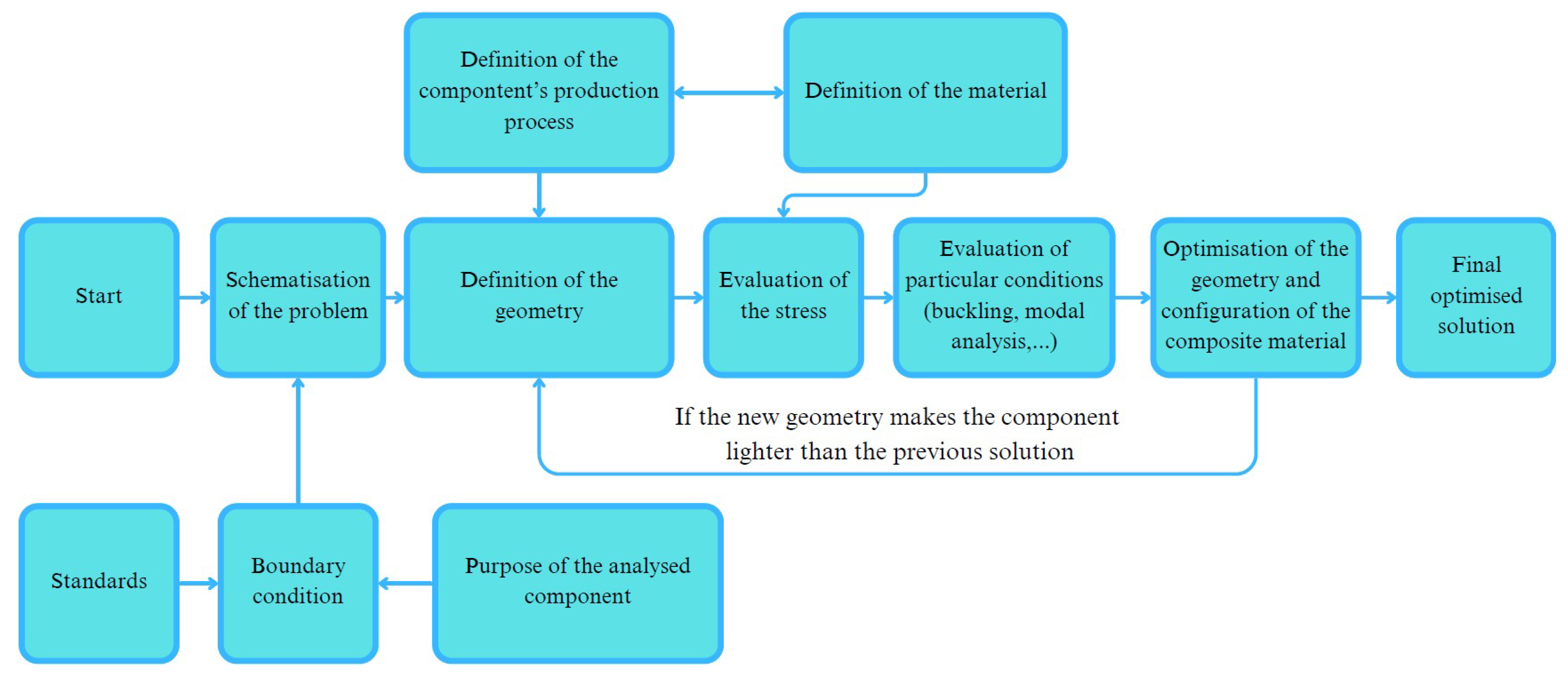
The design approach, aimed at reducing the weight of a component through the use of composite materials, can be summarized by the flowchart shown in Figure 1. After schematizing the problem, which depends on the boundary conditions, the geometry must be defined. This geometry is correlated with the manufacturing process of the studied component and the material selection. The stresses can then be determined through analytical, numerical, or experimental analysis, taking into account specific conditions. As an example of such specific conditions, in the automotive sector, the component experiences external vibrations, necessitating modal analysis to prevent resonance effects; additionally, buckling analysis is essential to ensure that the component not only endures the applied loads but also remains stable under certain conditions. Once a solution that satisfies all boundary conditions is found, the geometry optimization process begins. This is an iterative process that continues until the new geometry meets the required conditions. These boundary conditions typically depend on the purpose of the component being analysed or the applicable standards.

Figure 1.
Design approach flowchart.
2.2. Methods and Criteria Adopted
The case study must be analysed with respect to its boundary conditions and different configurations. Through the balance of momentum and angular momentum, the support reactions can be evaluated to determine the force distribution diagrams, which include tensile forces, bending moments, shear forces, and torques. Using these diagrams, the most stressed positions can be identified. After defining the geometry, the stress in the material can be analysed using De Saint Venant’s theory, Bredt’s formula, and Jourasky’s formula [19]. The stress profiles can be described using Equation (1):
where is the normal stress imposed by force F on the section area A, is the stress due to the bending moment at a distance y from the section’s centreline, is the bending moment, is the moment of inertia with respect to the centreline, is the stress from the torque, is the torque, is the mean area of the section, s is the profile thickness, is the shear stress, T represents the shear forces, and is the static moment of the section. This step identifies the worst-case scenario for the component, though a preliminary geometry must be established first based on material selection and production methods.
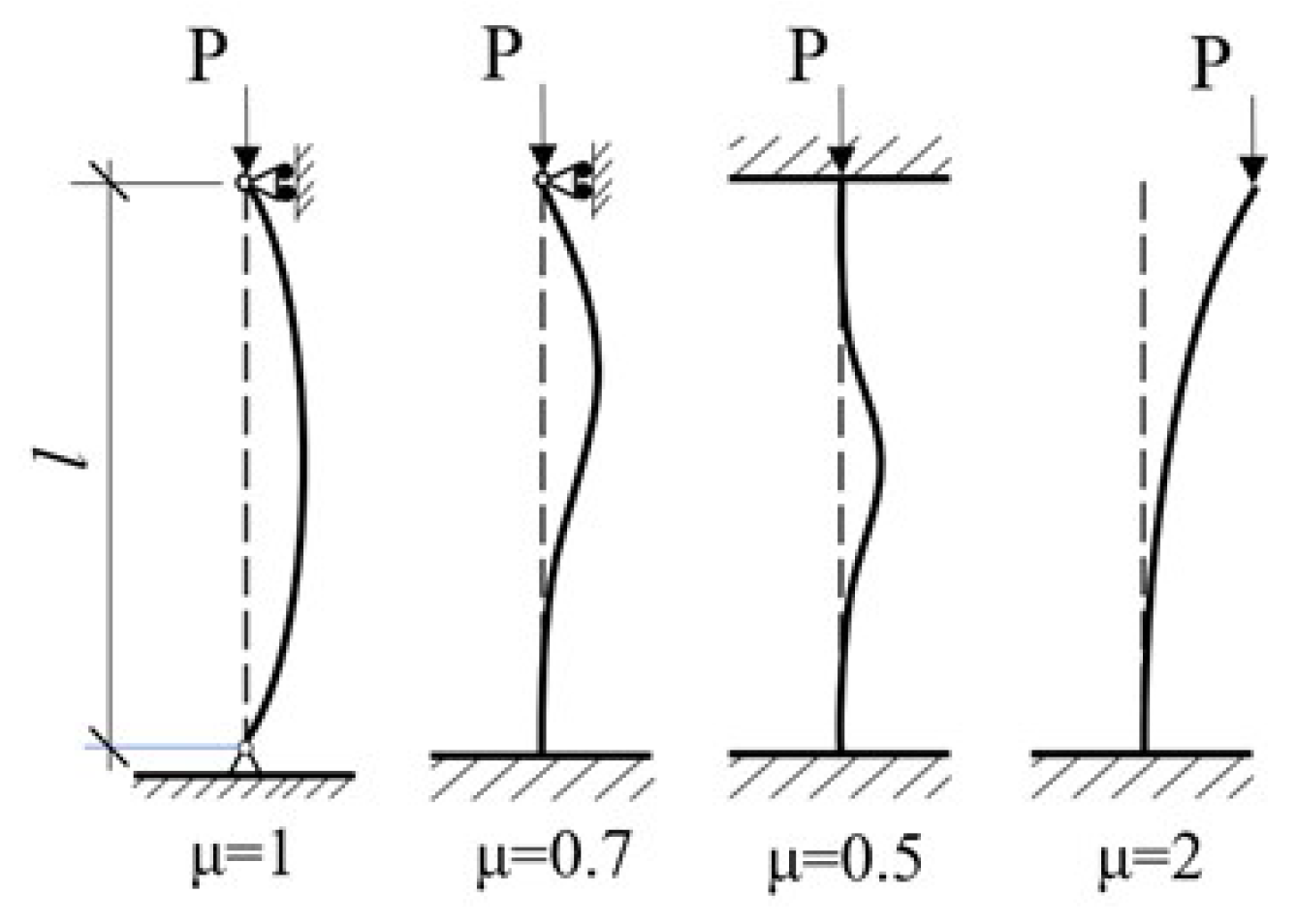
At this stage of the design process, buckling analysis must also be considered. Buckling refers to lateral deformations in structural elements subjected to compressive forces. In steel structures, where thinness is common, buckling is especially significant. According to elastic stability theory, Equation (2) defines , the critical load at which a perfectly elastic component begins to exhibit non-axial deformations:
where E is the Young’s modulus of the material, J is the section’s minimum moment of inertia, and is the length of free vertical displacement, which depends on the beam’s constraints. Usually, this value is the product of the beam’s length l and a correction factor . Figure 2 shows this value for different constraints.

Figure 2.
Different configurations and their values of .
Equation (2) assumes the load is perfectly applied at the section’s centre. However, in reality, this is not always achievable. Additionally, accidental material inhomogeneity, such as pre-deformed fibres, may result in a beam that is not perfectly straight. These are known as second-order effects [20], and to account for them, the criteria in (3) must be verified:
where is the axial failure force under a primary bending moment, is the buckling load at failure without a primary bending moment, is the equivalent bending moment along with the axial force, and is the ultimate bending moment at failure without an axial force. To define , Equation (4) must be used:
where A is the cross-sectional area, is the material’s yield strength, is the material safety factor, and is the reduction coefficient accounting for buckling. The factors and the dimensionless slenderness are defined in Equation (5):
where represents the effect of imperfections, with values of 0.13, 0.21, 0.34, 0.49, and 0.76 for curves , a, b, c, and d (European buckling design curves) respectively [20,21]. For the other terms in Equation (3), Equation (6) provides the method for evaluating them:
where and are the moments at the ends of the beam, and their ratio is negative for single-curvature bending and positive for double-curvature bending. The coefficient represents the plastic resistance modulus of the section, as defined in Equations (7) and (8).
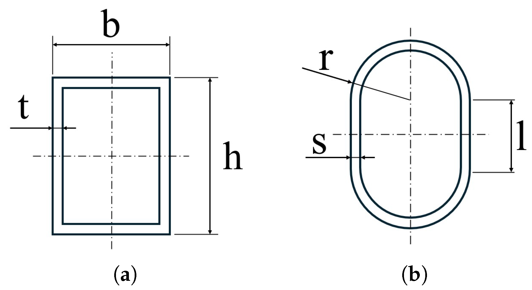
All the variables to evaluate the plastic resistance modulus of the section are the dimensions of the section itself. To understand them, Figure 3 shows the dimensions for a hollow rectangular section and for a hollow elliptical section.
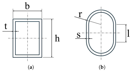
Figure 3.
Dimensions of the used sections. (a) Dimensions of the hollow rectangular section. (b) Dimensions of the hollow elliptical section.
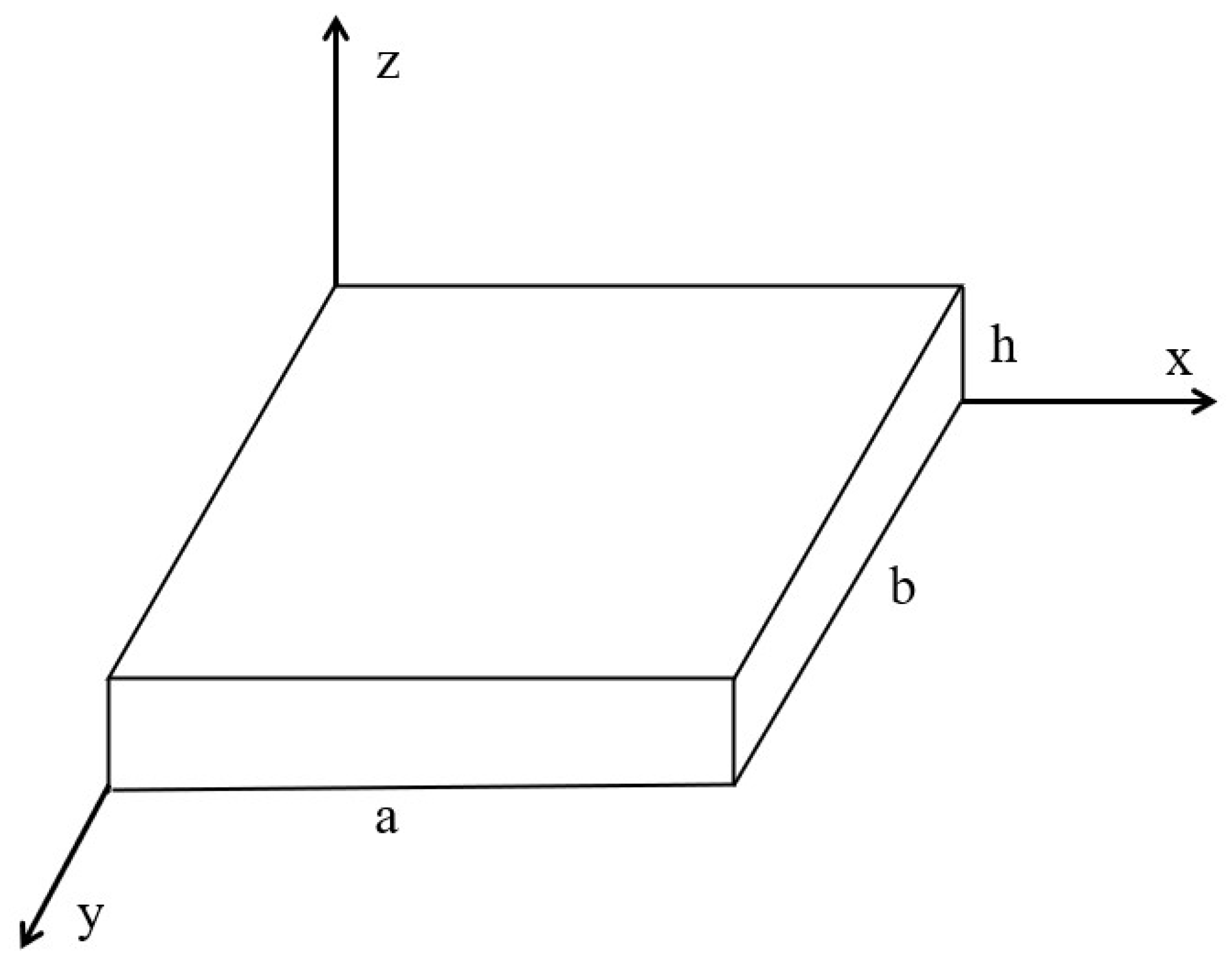
Given that the essence of this design methodology involves the utilization of composite materials, plate buckling [22] must be considered. Beginning with classical plate theory and incorporating laminated composite theory, a composite plate is examined, with its dimensions and coordinate system delineated in Figure 4:
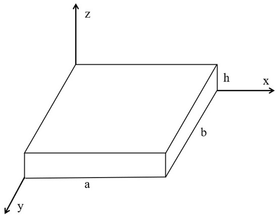
Figure 4.
Coordinate systems and dimensions of the composite plate.
The critical load for a slender composite plate subjected to uniaxial compression in the x-direction is articulated as delineated in Equation (9):
where is the critical buckling load per unit length (N/m) and b is the plate width. and are dependent on the components of the bending stiffness matrix and are obtained through Equation (10):
For a composite laminate, each value of the bending stiffness matrix can be determined through Equation (11):
where is the transformed reduced stiffness coefficient for each k-layer (see Equation (21)), is the coordinate of the upper surface of layer k and is the coordinate of the lower surface of the k-layer.
2.3. Choice of the Materials
Together with defining the geometry, the materials must also be selected. Most structural components in industrial vehicles are made of steel, an isotropic material with higher mechanical properties than other metals. This study aims to implement composite materials instead of metals due to their advantages in weight reduction. The choice of material depends on several factors: the availability of suppliers, the production process, the material’s performance in the studied scenario, and its cost compared to other options. A preliminary selection can be done thanks to Ashby’s diagrams [23], where the stiffness-density ratio helps to decide on a substitute for the material already implemented in the current solution but choosing in order to lighten the component.
To evaluate the mechanical properties of these materials, it is necessary to know the mechanical properties of both the fibre and the matrix, which are usually provided by suppliers. Assuming the fibres are aligned along the main longitudinal direction, Equations (12) and (13)—derived from the micromechanics theory of orthotropic plates [24]—can be used:
To determine the longitudinal compressive strength , the failure mode must be analysed. Naik and Kumar [25] evaluated the different analytical models to predict the longitudinal compressive strength and compared their predictions to experimental results. They identified that both Xu-Reifsnider [26] and Budiansky [27] models predict the compressive strength quite accurately when the parameter representative of the actual material system is ascertained properly. The first model predicted the compressive strength based on the analysis of microbuckling of a representative volume element using a beam on an elastic foundation model. The effect of matrix slippage and the fibre–matrix bond condition was included by two factors, namely, and . The final expression in terms of the constituent properties and micro-geometrical parameters is given by Equation (15):
where is the empirical factor representing matrix slippage, is the empirical factor representing fibre matrix bond and is the radius of fibre.
The second model unified the Rosen (based on microbuckling of the fibres) and Argon formula (based on the principle that the component of interlaminar shear stress due to the presence of misalignment produces kinking) for an elastic ideally plastic composite. The expression as given by Budiansky is defined by Equation (16):
where is the initial fibre misalignment angle in unidirectional composites and is the matrix yield strain.
The shear strength S and critical load are difficult to determine using formulas due to multiple uncertainty factors and the different behaviour of the matrix and fibre before failure [28,29]. Typically, this value is provided by the composite material supplier or can be evaluated through experimental tests such as single-fibre fragmentation testing, short beam shear, or the Iosipescu shear test [30].
Once the geometry of the component and the percentage of each type of ply are suggested, classical composite theory for two-dimensional laminates [24] can be applied for an initial analysis. By introducing a reference system with the first two axes on the lamina and neglecting the deformation (which is orthogonal to the lamina plane), the deformations of a specially orthotropic lamina can be evaluated using Equations (17) and (18). The components of the compliance matrix S are calculated from the lamina’s elastic constants:
To calculate stresses from deformations, the stiffness matrix Q (the inverse of the compliance matrix) must be used. These formulations can be applied to laminas with fibres reinforced along the primary axis. However, if there is a relative angle , the rotation matrix T must be used, where and , as described in Equation (19):
To adapt the compliance matrix S and the stiffness matrix Q to the new direction, the following Equation (20) must be applied:
Furthermore, the expression for calculating stresses in a generic lamina becomes the one described in Equation (21):
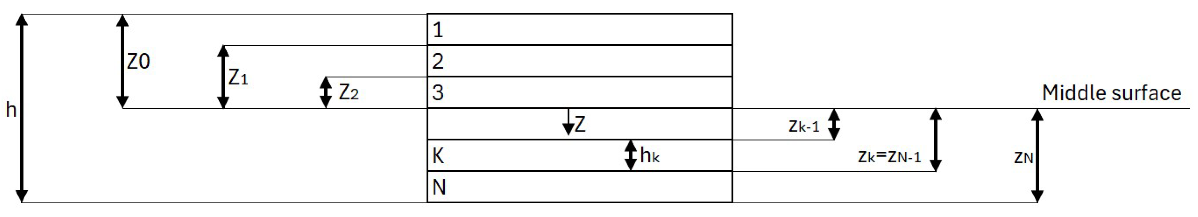
To obtain a first approximation of the deformation values, the extensional stiffness matrix A must first be derived. By setting the total number of laminas N and the composite thickness h, a coordinate system can be defined (as shown in Figure 5), and then A can be evaluated using Equation (22):
where i represents the rows of the matrix, j the columns, and k the number of layers. Additionally, a local reference system has been defined to evaluate stresses. Using the deformation values, obtained analytically by multiplying the inverse of the A-matrix with the stress matrix (calculated using Equation (1) and the laminate thickness), it is possible to use Equation (23) to calculate the local stresses along each lamina’s directions within the entire laminate:
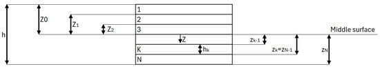
Figure 5.
Coordinate system for the position of laminates.
By relating the local reference system to the lamina’s system, and considering the maximum bending stress and maximum shear stress (obtained from the component’s geometry and boundary conditions), it is possible to apply the Tsai–Hill criterion, described in Equation (24), or the maximum stress criterion, described in Equation (25), based on the material resistance values.
where represents if > 0 or if < 0, while represents if > 0 or if < 0. To determine if the ply will theoretically fail, the factor of safety (FOS) must be less than 1.
Finally, to increase resistance to weathering or sunlight, a protective film described by Komartin et al. [31] or Zhang et al. [32] should be applied to the surface of the component.
2.4. Optimization of the Geometry
After deciding on the material and verifying the boundary conditions, the geometry of the section must be chosen. Since weight reduction is the main goal of the research, it is preferable to select a hollow section rather than a solid one. Furthermore, the shape of the vehicle components also depends on the production process, which is related to the material. When working with composite materials, optimizing the geometry and designing the material itself must be done simultaneously, thanks to the flexibility in choosing different fibre orientations.
The idea is to develop objective functions that need to be minimized or maximized, depending on the goal of the design. These functions could represent the mass of the component or its cost. The variables in the function are the parameters describing the geometry, such as the main dimensions and thickness. The process must adhere to a system of constraints, which are typically imposed by standards or safety factor requirements for the section under analysis.
To illustrate this concept, Figure 6 shows an example: with the weight of the component as the objective function (dependent on its thickness), the goal is to minimize it without exceeding the current configuration’s weight and ensuring a safety factor greater than 1. Another constraint is related to the production process, meaning the thickness must be an integer. In this scenario, the optimized solution has a thickness of 6 mm.
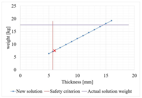
Figure 6.
Example optimization chart: here the thickness of a hollow section has been optimized, with the weight reduction as the main goal. Two boundary constraints are shown, one defined by the safety criterion and one defined by the previous solution.
This is a simple example; in practice, objective functions, parameters, and constraints can be much more complex.
The algorithm adopted and, most of all, the variables in this process depend on the needs of the user. In the literature, an extended review [33] about the implementation of an optimization algorithm for laminated composites is presented: the algorithms suggested are the meta-heuristic ones (such as Genetic Algorithm, Simulated Annealing algorithm, Particle Swarm Optimization, Ant Colony Optimization, Firefly Algorithm), which are more popular due to their efficiency and stability. It was also described that stacking sequence and geometry are considered the key design variables in optimization problems, and in most of the articles, the main goals were the following:
- Minimizing the weight;
- Maximizing the mechanical properties;
- Minimizing the cost of the component.
As an example, in the following scenarios, an objective function that can be taken is the minimization of the weight (which is correlated here to the minimization of the costs), and the Tsai–Hill criterion and maximum displacement can be chosen as constraints. The variables in this research work should be the geometry of the component and the stacking sequence.
3. Implementation of the Design Approach: The Front Underrun Protection Device
3.1. Description of the Component
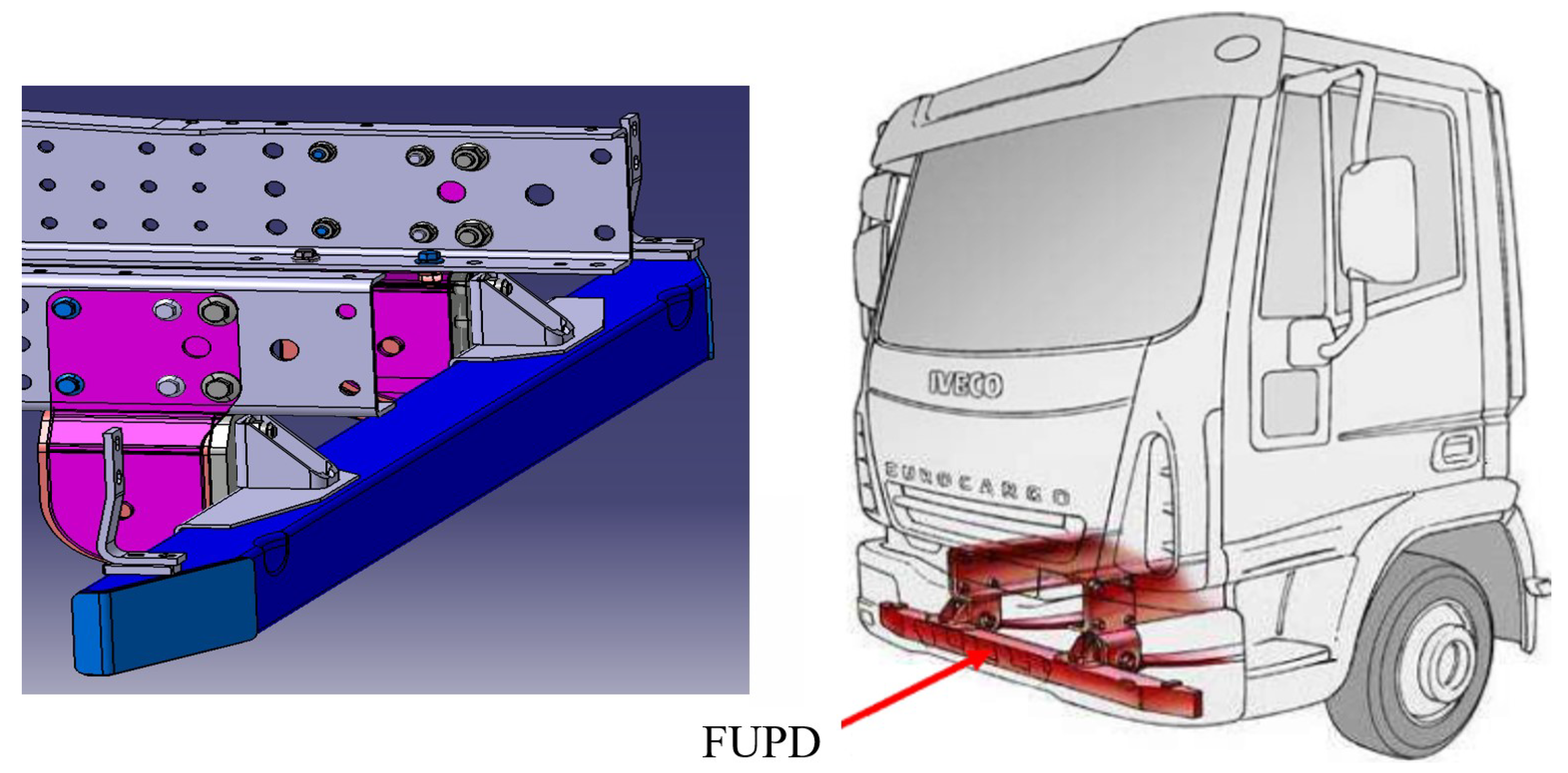
The front underrun protection device (FUPD) is a component installed on heavy industrial vehicles designed to limit the damage caused to cars in the event of a collision. In the case of a collision between a heavy vehicle and a car, there is a risk that the car may become wedged beneath the heavy vehicle. To prevent this, the underrun protection device was introduced in the position shown in Figure 7. This component was chosen as an applicative example, but the lightweight process of the FUPD is part of a larger project that aims to reach a weight reduction for each component of an industrial vehicle—some of which have already been completed by the authors [18,34].

Figure 7.
On the left, a 3D view of the studied device; on the right, the location of the FUPD on the industrial vehicle.
The FUPD design needs to meet some requirements to ensure its functionality:
- Be compliant with the United Nations Economic Commission for Europe (UN/ECE) standard n.93 [35];
- Exhibit natural frequencies higher than the characteristic internal and external excitation frequencies of the vehicle;
- Prevent buckling of the structure.
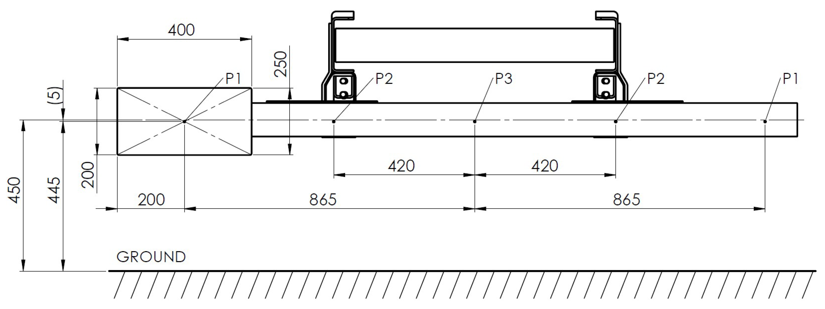
This study focuses on the Eurocargo 120EL category of Iveco® vehicles, which have a maximum weight of 120,000 N, approximately 12,000 kg. UN/ECE standard n.93 [35] outlines the methodology to homologate the analysed component. Three loading conditions are defined: P1, P2, and P3. Forces P1 and P3 must be equal to half the weight of the vehicle at its maximum load, while force P2 must be equal to the entire weight of the vehicle. For a vehicle weighing 12 tons, P1 = P3 = 60 kN and P2 = 120 kN. These forces should be applied longitudinally to the chassis, following the positions illustrated in Figure 8, with an almost static application velocity as defined by the standards.
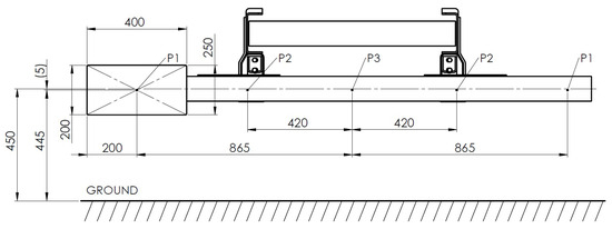
Figure 8.
Geometry and location of the three different loads P1, P2 and P3 [mm].
The loads are applied through a plate positioned between the piston rod and the FUPD surface, with the central point of the plate aligning with the positions described for the loads. The success of the homologation test is determined by ensuring that the maximum displacement of the FUPD is less than 400 mm from the outermost surface of the bumper. Plastic deformation of the component is allowed, but it must not exceed the maximum deflection outlined in the regulations. For composite materials, known for their brittleness, only elastic deformation is acceptable. Any other type of deformation would result in the component being deemed broken and ineligible for homologation.
Figure 9 shows where the force is applied. The dimensions are = 865 mm, b = 400 mm (so a = 465 mm), and F = 60 kN. Using momentum and angular momentum balance, the support reactions are evaluated through the system of equations in (26).

Figure 9.
Sketch of the component treated as a beam.
Based on these data, we calculate = 98.875 kN and = −34.875 kN.
Next, force distribution diagrams are determined. Considering that the device must be no more than 400 mm from the ground and that the beam is 100 mm high, the centreline of the bar is 450 mm from the ground. The load is applied 445 mm from the ground [35], resulting in a torque moment with a 5 mm lever. The torque = 300 Nm.
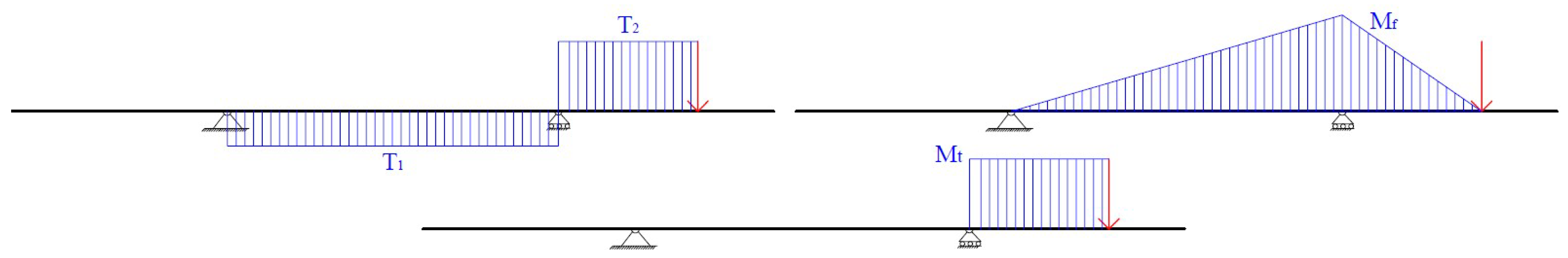
The force distribution diagrams are shown in Figure 10, indicating that the most critical section is where the support reaction is applied. The bending moment is = 27,900 Nm, with = and = F.
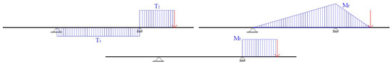
Figure 10.
Force distribution diagrams of the analysed component.
The P1 load [35] was analysed as the most critical of the three loading conditions described in the European Standard due to the highest bending moment on the supports. Specifically, = 27,900 Nm, = 0 Nm, and = 24,000 Nm. P2 is more critical for the brackets linked to the chassis, where the constraint reaction would be 120 kN instead of 98 kN.
These loads are then used to analyse the structural integrity of the FUPD. In addition to this, a modal analysis is needed to evaluate the natural frequencies and corresponding mode shapes of the structure. Indeed, external excitation and internal power sources, such as engine vibration excitation and road excitation, are the sources of frame resonance. Road vibration frequency of cars is in the range of 0–100 Hz [36] and the vehicle body’s first order vibration frequency needs to be higher than 20 Hz, considering the most important road excitations are within this frequency [37]. Equation (27) can be used to determine the excitation frequency of diesel engines, according to pertinent research:
where is the number of engine strokes, z is the number of engine cylinders, and n is the engine speed, defined in RPM. A six-cylinder, four-stroke diesel internal combustion engine is used in this design of the truck, and for the calculation, a rated speed of 2500 RPM is chosen in order to be in a critical situation. After these considerations, when moving, the diesel engine vibrates at a frequency of 125 Hz.
Three different configurations of the analysed component were studied: the traditional steel S460Q design, a glass-fibre-reinforced polymer (GFRP) option, and a carbon-fibre-reinforced polymer (CFRP) alternative.
3.2. Traditional Solution
The properties of the traditional steel configuration, also defined as S460Q according to UNI EN 10027-1, are shown in Table 1. This material was adopted both for the FUPD and for the supports, which were welded to each other.

Table 1.
Mechanical properties of S460Q.
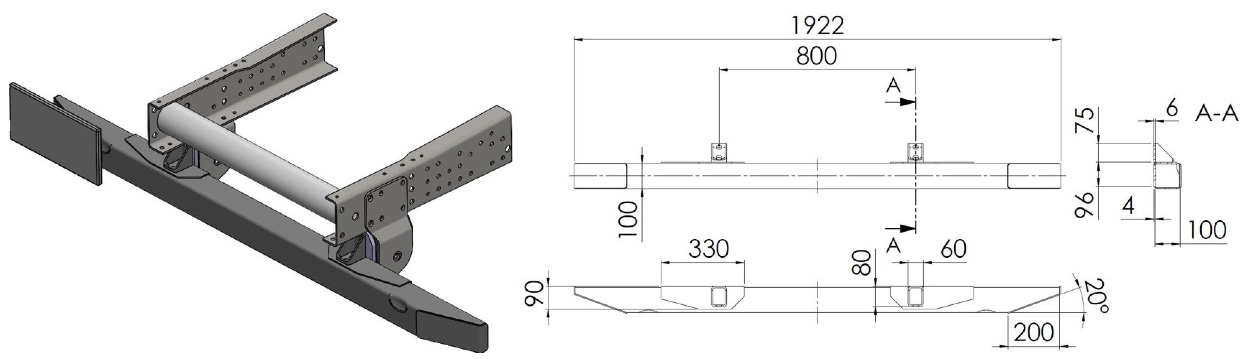
Figure 11 shows the geometry of the traditional component design. In this solution, the stress = 498 MPa, assuming = 2.801 × 106 mm4, which is the moment of inertia related to the section where is maximum. The action of the reinforcement bracket is added to that of the bar, resulting in = 5.15 MPa and = 231.74 MPa.

Figure 11.
Current solution [mm].
The tensile stress in the critical section is higher than the yield stress of the material but lower than the ultimate tensile strength (620 MPa), making this value acceptable as a preliminary estimate. To study displacements, equations of the elastic line [19,38] were applied. Solving the system reveals a maximum displacement of 16.83 mm, well within the target range, where the maximum allowable displacement is 81 mm, considering the imposed standards and the vehicle’s geometry.
3.3. GFRP Innovative Solution
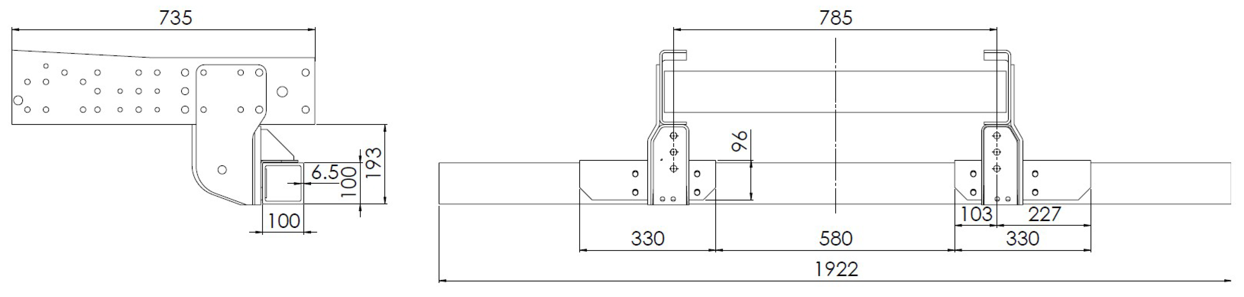
Figure 12 shows the GFRP geometry for the initial study, where the cross-section is a square profile with a 6.5 mm thickness. The reason behind the choice of this material was mainly for the availability of the supplier but also factors such as the mechanical properties of the material and its cost related to the feasibility of high production volumes influenced the decision. Regarding the material of the supports, steel S460Q was adopted in this initial configuration. This configuration was used to compare numerical results from FEM analyses with experimental tests. Concerning the material of the supports, steel S460Q was adopted in this initial configuration. Given that the material and production process are typically chosen together to accommodate high production volumes (estimated at 6000 units per year), pultrusion [39] was selected as the manufacturing process, adopting the unidirectional fibre as the architecture of the material structure. An isophthalic polyester resin was chosen as the matrix, being a common choice with this production process [40]. The minimal mechanical properties of this material, given directly by the supplier and according to UNI EN 13706-3, are shown in Table 2: presuming the material demonstrates brittle behaviour, the stress–strain response was considered linear-elastic, defined by the chosen modulus of elasticity. Failure was characterised as occurring upon reaching the tensile strength, in accordance with the literature [41,42]. The same logic was applied to the CFRP solution.
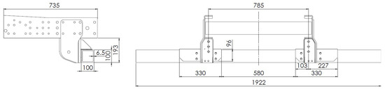
Figure 12.
First GFRP assembly developed [mm].
Table 2.
Mechanical properties of GFRP.
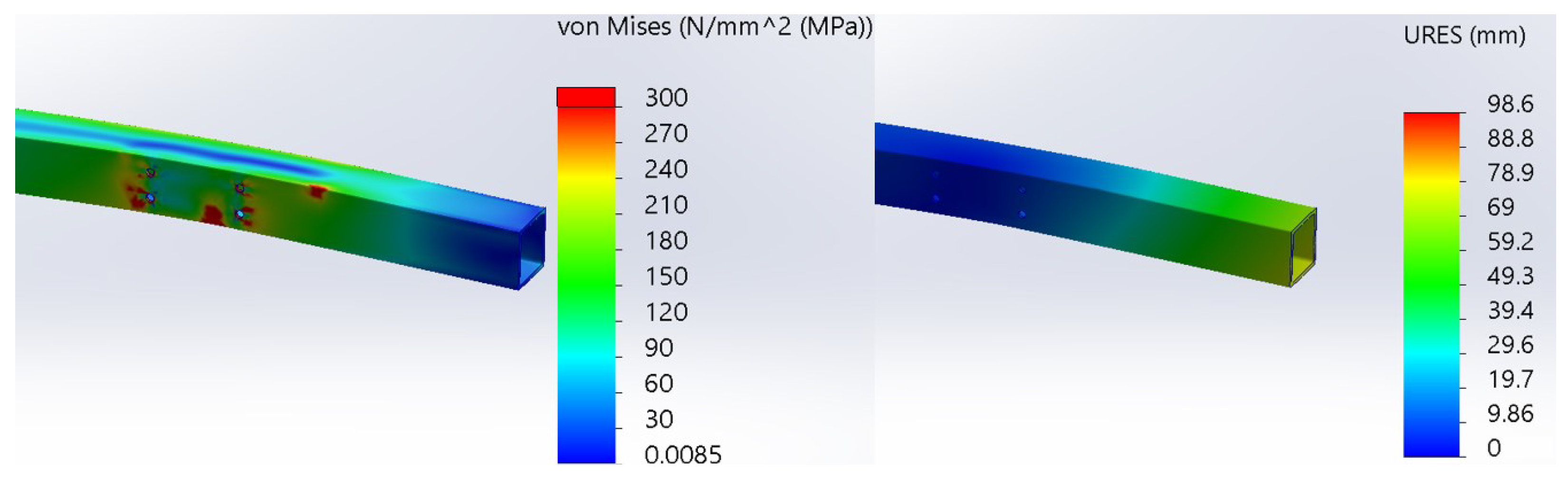
Simulations of this configuration were run in Solidworks®, using a solid mesh based on curvature with 265,786 nodes and 135,015 quadratic tetrahedral elements. The final mesh resulted from an h-refinement procedure that concentrated on the FUPD and its supports. It was defined using a chassis with a coarser mesh to conserve computational time and resources. A static analysis was conducted to confirm the numerical model prior to investigating additional properties of the examined component, including resonance frequencies, and subsequently discovered buckling modes. Regarding the connections of the chassis components, bonded interactions were utilised, as the chassis is not the focus of this research paper. Conversely, bolt connections were employed for the connections between the FUPD, brackets, and other components to accurately simulate the actual connections among these parts, except for the plate where the force is applied, where a bonded interaction is chosen to avoid a possible rigid motion of the body. The mechanical properties of the composite material were implemented by the software through the definition of a local reference system and the material’s orthotropic behaviour. The local reference system is chosen based on the mechanical properties of the material, so the X-axis was the longitudinal axis along the FUPD, while the Y-axis was the transversal axis on the surface of the beam. The Z-axis defines the dimension of the thickness of the FUPD. Regarding the orthotropic behaviour, the mechanical properties of Table 2 were added in the definition of the material. This numerical test showed that the most stressed area of the FUPD is the rear surface, specifically the inferior edge, as illustrated in Figure 13.

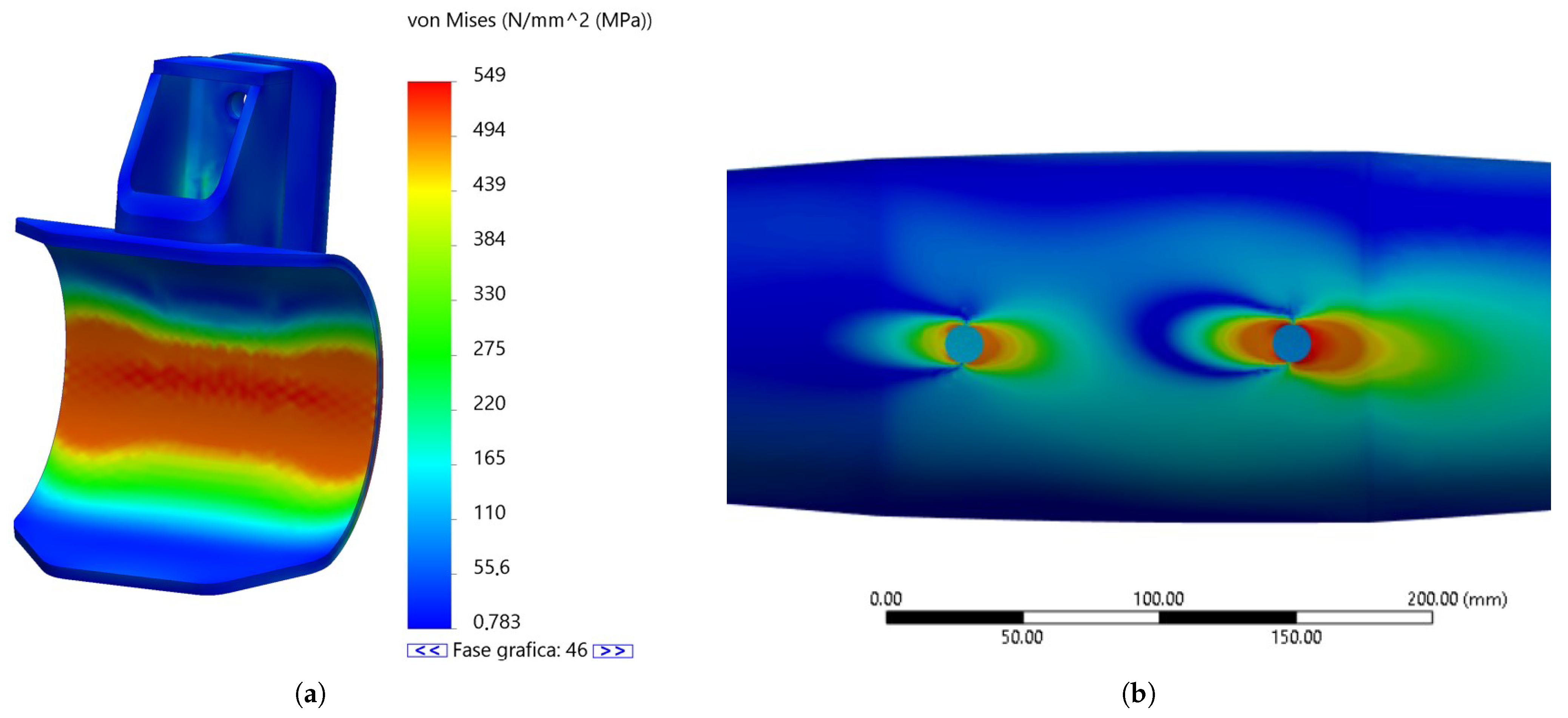
Figure 13.
Results of the GFRP first solution at the load application end: on the left is the Von Mises stress, while on the right is the total displacement. It is clear that the component has reached the failure point in some areas.
The most critical stress is the shear stress, which, combined with the longitudinal compressive stress near the side of the support close to the applied load, leads to component failure. The numerical test also identified other highly stressed areas near the bores where the supports are linked to the bar, exceeding the tensile strength of the GFRP material.
To verify the numerical computations, an experimental test was conducted using the 100 × 100 profile with a 6.5 mm thickness. A system was developed to represent a real vehicle, where the chassis was attached to simulate a fixed support 735 mm behind the front edge, as shown on the left of Figure 14. The FUPD was mounted 400 mm from the ground, matching the conditions of the numerical analysis. On the right of Figure 14, a hydraulic cylinder was used to apply the load, pushing on a plate aligned with the concentrated load. This force is applied directly to the beam and not its supports. The plate was linked to the cylinder via a hinge, allowing it to follow the component’s deformation.
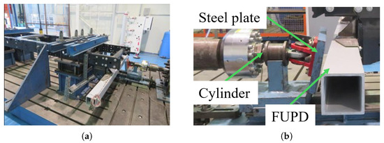
Figure 14.
Photos of the experimental test area. (a) Setup for the experimental test on the studied component. (b) Zoom of the cylinder used to apply the loads.
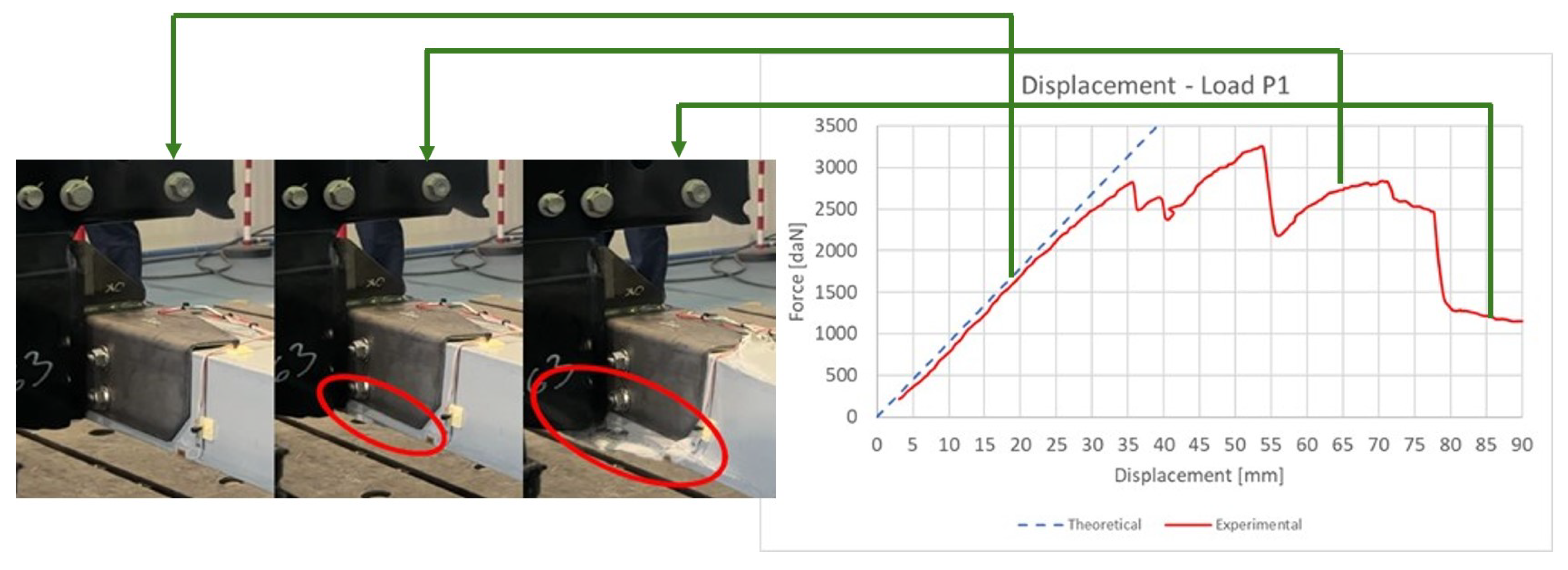
As expected, the test showed that the FUPD failed, as represented in the load-displacement diagram in Figure 15, accompanied by images of the failed area.

Figure 15.
On the (left), a zoom on the failed area of the FUPD (circled in red), and on the (right), the diagram of load versus displacement from the experimental test.
The graph shows that failure occurred at F = 28.11 kN with a displacement of 35.74 mm, the final value on the red line near the theoretical straight line. Afterwards, the load increased due to the steel reinforcement, followed by a collapse of the force curve. However, Figure 15 reveals that the failure was not caused by axial stress from the bending moment but by shear stress on the rear surface of the beam, near the steel reinforcement.
The Tsai–Hill criterion was applied to determine the factor of safety (FOS) for the composite material. Using the FOS from the numerical analysis, the failure load was evaluated and compared to the load reached in the experimental test.
Table 3 shows the minimal difference between the numerical and experimental results, which is less than 5%. The FOS from the numerical computation was taken at the critical edge of the component (Figure 15), while the experimental FOS was obtained by dividing the actual load by the rated load.
Table 3.
Comparison between the FEM model and the experimental data.
Given the strong correlation between the numerical and experimental values, a GFRP model of the FUPD was developed that can withstand the stress imposed by European regulations. The geometry of the new solution is shown in Figure 16.
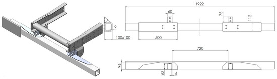
Figure 16.
Final GFRP assembly developed [mm].
The new solution has a similar geometry to the previous one, but the FUPD thickness was increased to 9 mm, and the reinforcement bracket was modified as shown in the drawing. The new configuration, particularly the “C” profile replacing the original “L” profile, was chosen to reduce shear stresses on the rear surface of the FUPD, as previously explained.
The reinforcement brackets were made from aluminium 7075-T6 [43], selected for its lighter density and mechanical properties comparable to steel, as shown in Table 4:
Table 4.
Mechanical properties of Al 7075-T6.
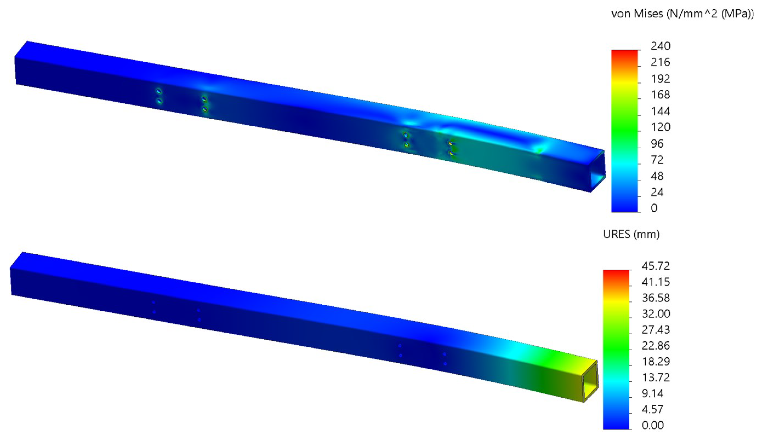
The results confirm that the FUPD withstands the applied load: the Von Mises stress is lower than the ultimate strength of the GFRP, and the displacement is within the limit imposed by the standard, as shown in Figure 17.

Figure 17.
Final GFRP assembly stress: the Von Mises stress is shown at the top, and the total displacement of the FUPD is shown at the bottom.
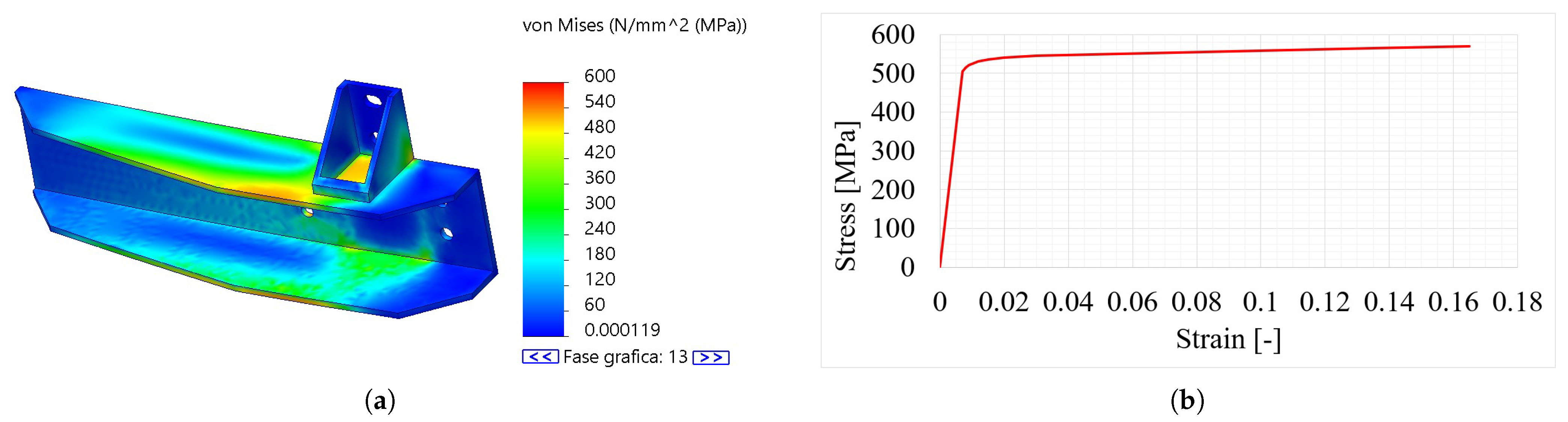
Due to the higher stress on the brackets exceeding the yield stress of the material, a non-linear analysis was performed. To reduce computational costs, the fitting radii of the brackets were not considered in this analysis, but this simplification did not affect the most stressed areas. The simulation was set as a non-linear, static analysis with iterations based on the Newton–Raphson technique, through displacement control, due to the almost plateau of the aluminium after the yield point. As shown in Figure 18a, the FEM analysis results demonstrate that the tensile stresses on the bracket are lower than the ultimate strength of the material. In Figure 18b, the stress–strain curve of the 7075-T6 aluminium alloy adopted for the non-linear analysis is presented.
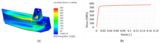
Figure 18.
Non-linear FEM analysis on the innovative aluminium bracket. (a) Von Mises stress results from the non-linear analysis of the bracket. (b) Stress–strain curve of 7075-T6 aluminium alloy at quasi-static strain rate.
As explained previously, modal analyses were performed: Figure 19 shows that the first natural frequency of the structure is far from the highest excitation that the FUPD is subjected to.
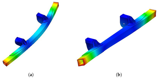
Figure 19.
Modal analysis of the GFRP solution. (a) First resonance mode of the GFRP solution: the resonance frequency here is 158 Hz. (b) Second resonance mode of the GFRP solution: the resonance frequency here is 181 Hz.
Global and local buckling were also studied. Figure 20a shows the first global buckling mode of the GFRP solution, with a safety factor of 9.09, while Figure 20b shows the first local buckling mode, with a safety factor of 7.21.

Figure 20.
Buckling analysis of the GFRP solution. (a) First global buckling mode of the GFRP solution. (b) First local buckling mode of the GFRP solution.
3.4. CFRP Innovative Solution
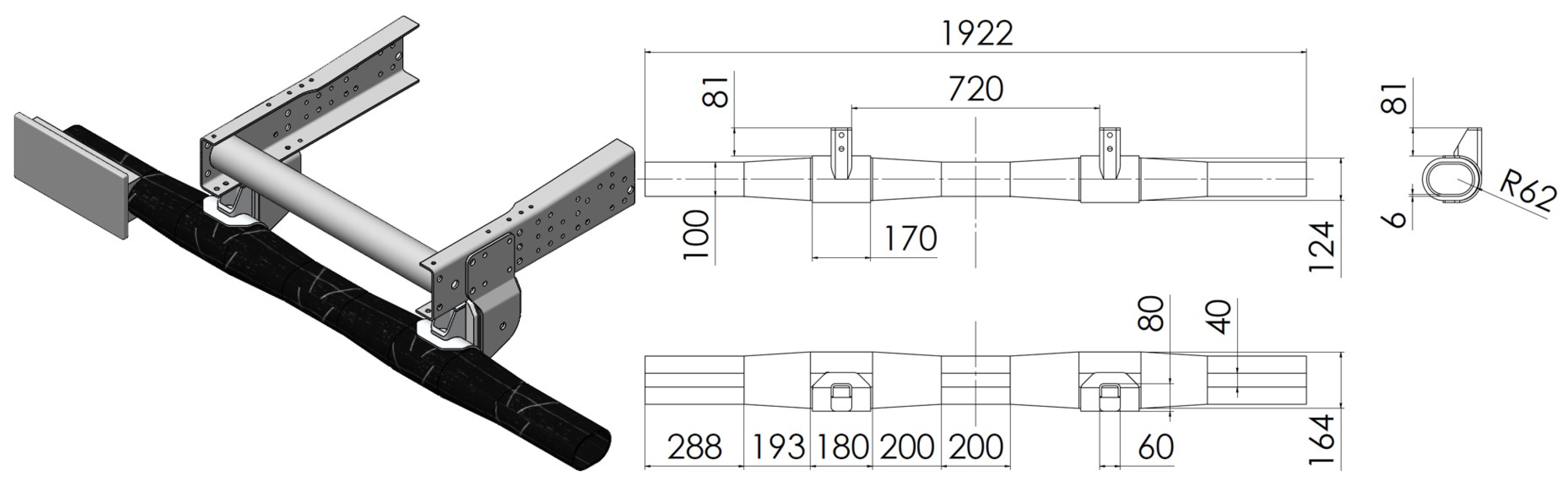
The last solution studied was designed using carbon-fibre-reinforced polymer (CFRP). The selection of this material was the result of a compromise between the highest mechanical properties as possible while maintaining an affordable increment on the costs of the component. For this material, the FUPD was manufactured using a process called filament winding [39], adopting the unidirectional fibre as the architecture of the material structure. With this production method, a different geometry was applied, as shown in Figure 21. The new geometry features the innovative elliptical profile where the cross-section is not constant, but the overall length remains the same as the GFRP profile. The decision to alter the section at the points of support was primarily made to increase resistance in those areas.
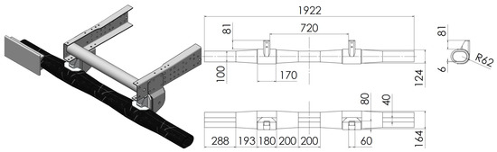
Figure 21.
CFRP assembly developed [mm].
Furthermore, the connection between the FUPD and the supports was modified, utilizing a support structure that can adapt to the new geometry and is made of the same material, as described in Table 4. In this configuration, the supports were designed to position the FUPD 5 mm lower, which avoids the torque moment described in Section 2.1. In the previous solution, this adjustment was not possible due to the similarity of the existing supports, but with the new design of the component, it became feasible. It should be noted that the experimental testing performed on the GFRP solution facilitated the development of a numerical model that closely approximates reality. Upon establishing the model’s reliability, it was deployed for various geometries and materials.
The carbon fibre chosen for this study is M50J [44], and the matrix is an epoxy resin (the epoxy resin is commonly used with this production process [40]) SX10 [45], with their mechanical properties detailed in Table 5. For the properties of the ply, see Table 6, evaluated through the equations of Section 2.3.
Table 5.
Property of the M50J carbon fibre and SX10 epoxy resin.
Table 6.
Mechanical properties of CFRP.
After testing various configurations, the analytical studies determined that the optimized solution, with the described geometry, has a thickness of 6 mm and consists of 20 layers (with each ply having a thickness of 0.3 mm). The Layer Stacking Sequence (LSS) includes 35% of the plies oriented at 5°, 35% at −5°, 10% at 45°, 10% at −45°, and 10% at 90° made by filament winding as already done for a hydraulic cylinder [46]. This result was achieved through an optimization process where the main constraint was the Tsai–Hill criterion, and six variables were chosen: the thickness of the section and the percentage of plies in five specific orientations (5°, −5°, 45°, −45°, 90°), selected based on the adopted production process and to maximise strength in the main directions. The function to be minimised was the weight; therefore, the minimum thickness was selected (as it is a variable directly related to the weight). Once a solution was found, an FEM simulation was performed to confirm the LSS and the previously determined thickness. Numerical analysis shows that the studied device can withstand the application of force P1: as shown at the top of Figure 22, the maximum displacement is around 36 mm, which is below the limit imposed by European regulations.
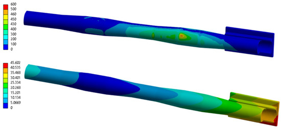
Figure 22.
CFRP assembly results: at the (top), the Von Mises stress of the component is presented, while at the (bottom), the total displacement is shown.
The study of this configuration was conducted using Solidworks® for 3D modelling and Ansys® for simulations. A solid mesh was used, based on curvature, with 424,821 nodes and 391,808 total elements. The type of solid elements used varied by component; for the FUPD, linear hexahedral elements were used. The software incorporated the mechanical properties of the composite material by establishing a local reference system and defining the material’s orthotropic behaviour. The local reference system is selected according to the material’s mechanical properties, designating the X-axis as the longitudinal axis along the FUPD and the Y-axis as the transverse axis on the beam’s surface. The Z-axis delineates the dimension of the FUPD’s thickness. Each element here represents a segment of the ply, characterised by a finer mesh, which results in augmented computing time, while also accounting for the interactions among each ply. The mechanical properties from Table 6 were incorporated into the specification of the material about its orthotropic behaviour. At the bottom of the same figure, the Von Mises stress of the FUPD is displayed: the most stressed area is at the closest support to the applied load. The stress is less than 410 MPa, meaning the component remains within safe limits due to the material chosen.
A non-linear static analysis for the brackets was also performed under load P2. The results, shown in Figure 23a, indicate that the maximum Von Mises stress in the support is around 550 MPa, which does not exceed the failure threshold.

Figure 23.
Numerical analysis for the supports of the CFRP solution. (a) Nonlinear analysis results on the bracket. (b) Von Mises stress of the FUPD solution in CFRP with bolt connections to the brackets.
In this design, the connection between the brackets and the FUPD is made using an epoxy adhesive, as described by Konchakova et al. [47], instead of traditional bolts. This decision was made to avoid excessive stress concentrations around the bolt holes. Figure 23b shows a zoomed-in view of the Von Mises stress graph for the FUPD’s linked area, revealing a stress peak near the holes. While the plies can withstand stress along the fibre’s longitudinal direction, the FUPD could fail in that area because not all plies share the same orientation. To verify this, it was found that the contact area between the tubular section and the supports is around 10,000 mm2, and the P2 load is 120,000 N, as required by European standards. The shear stress in this area is around 12 MPa, well below the stress limit for Konchakova’s adhesive epoxy, as well as the in-plane and interlaminar shear strength of the composite material.
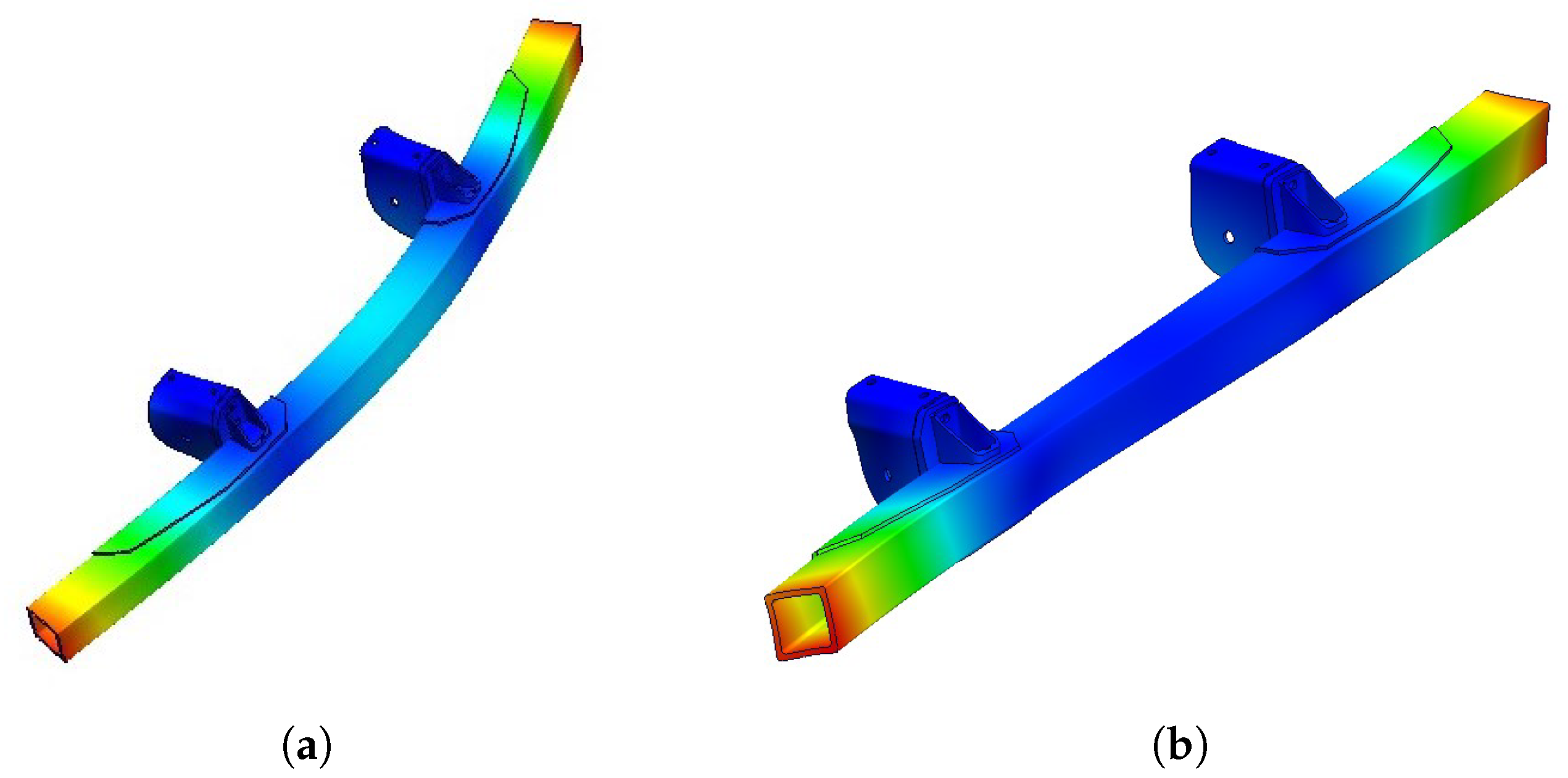
Modal analyses were also conducted: Figure 24 shows the first and second resonance modes of the structure. With the same considerations of Section 3.3, it is clear that the component does not reach the resonance, having different frequencies than the external and internal excitations of the structure.
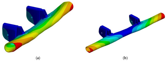
Figure 24.
Modal analysis of the CFRP solution. (a) First resonance mode of the CFRP solution: the resonance frequency here is 277 Hz. (b) Second resonance mode of the CFRP solution: the resonance frequency here is 289 Hz.
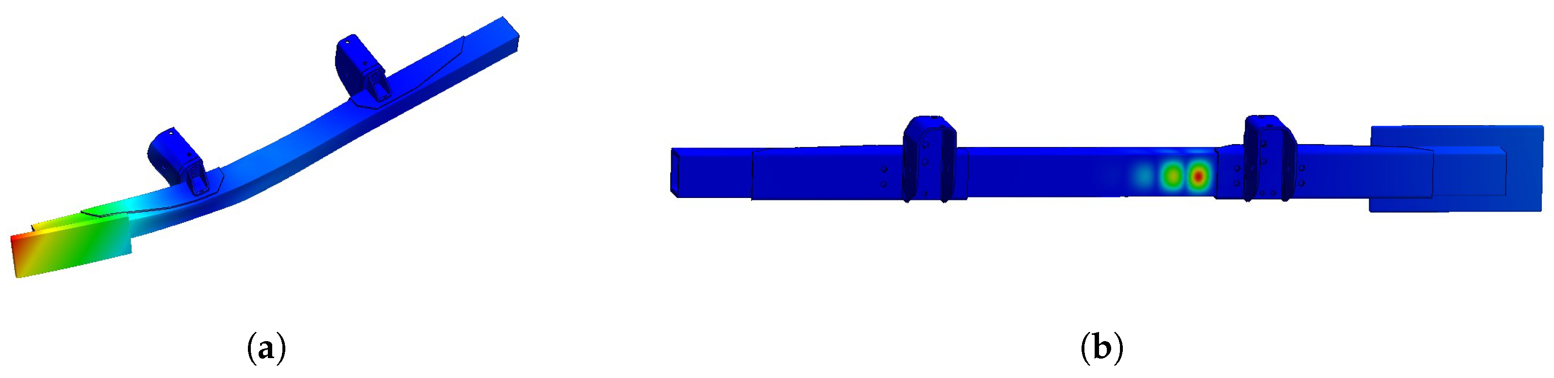
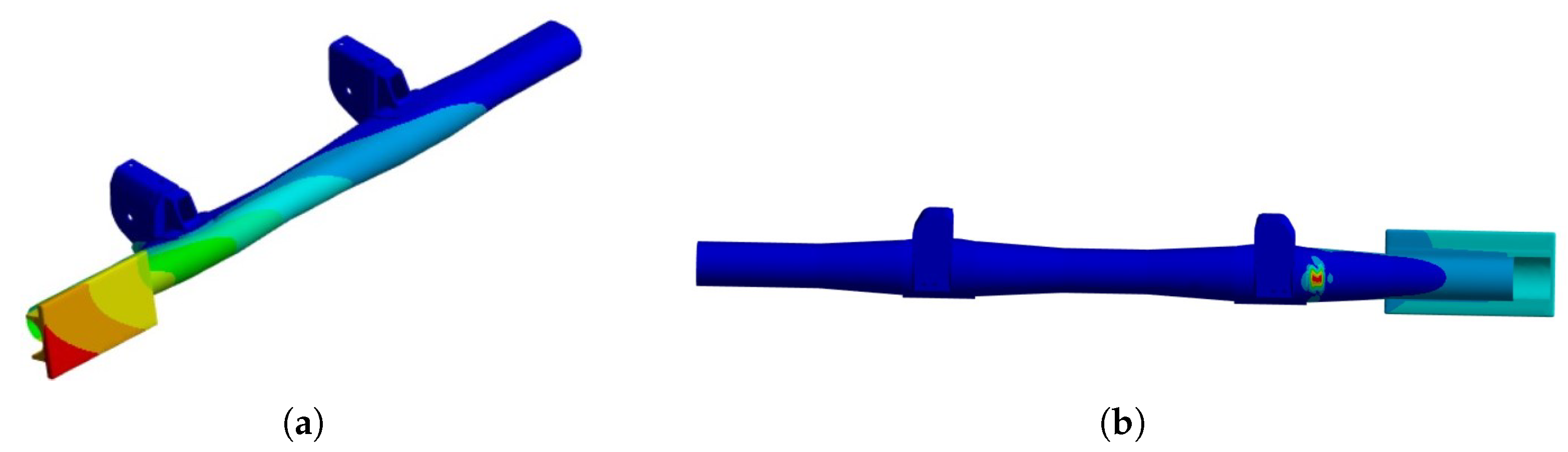
For the buckling analysis, Figure 25a shows the first global buckling mode of the CFRP solution, with a safety factor of 9.85, while Figure 25b shows the first local buckling mode, with a safety factor of 10.82.

Figure 25.
Buckling analysis of the CFRP solution. (a) First global buckling mode of the CFRP solution. (b) First local buckling mode of the CFRP solution.
4. Discussion of the Results
Using data from manufacturer datasheets and the FEM program’s 3D models, the mass of the FUPD and the supports for each configuration were determined.
Table 7 presents the weights of the FUPD in the three configurations studied. The percentage of weight reduction (W) and the percentage increase in cost (c) were evaluated as described in Equation (28):
Table 7.
Costs and weights of the different solutions.
A clear reduction in weight can be seen when comparing the steel solution to the composite material solutions: the glass fibre solution shows a 17.7% reduction in weight compared to the steel solution, and the carbon fibre solution shows a 55.6% reduction. However, the cost comparison reveals that the new FUPD and support designs require a greater initial investment. The cost difference between the innovative solutions and the traditional one is approximately EUR 17.68 for the GFRP solution and EUR 393.95 for the CFRP solution (after subtracting the cost of the traditional FUPD). Nevertheless, considering the economic savings from reduced fuel consumption, the time required to recover the initial investment is less than 5 years for the CFRP solution and less than 1 year for the GFRP solution, as illustrated in Figure 26. The calculations assume a vehicle lifetime of 11 years and an average mileage of 1.49 million kilometers [48], or 135,000 km per year.
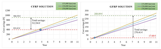
Figure 26.
Graphs of the amortization for the two innovative solutions.
An estimate of annual fuel consumption was made for both the traditional and optimized solutions, with a reduction of approximately 41.21 L/year for the CFRP solution and 13.09 L/year for the GFRP solution, as shown in Table 8. Based on these results, it was possible to estimate how fuel consumption reductions can impact both economic savings and CO2 emission reductions. This calculation was made using data on diesel engine performance, as diesel is the most common fuel for industrial vehicles. The economic savings were calculated based on the current fuel price of 2 EUR/L (the average price in Italy during early 2024).
Table 8.
Evaluation of the economic savings and reduction in CO2 emissions.
5. Conclusions
This research demonstrates a design approach for an industrial vehicle component using composite materials. The analysis began by studying the applied loads, optimizing the geometry to distribute stresses along the component, analysing resonance modes, and considering types of instability. Once the materials were defined, the results were evaluated, and the component’s geometry was optimized using specific algorithms. To consolidate the procedure, two case studies—one with GFRP and one with CFRP—were presented, focusing on the economic aspects of these optimized solutions. As shown in earlier sections, this process is not a linear flowchart due to the many variables involved. The ability to modify both the geometry and material configurations allows for alternative solutions, verified for the scenario under study.
The solutions can be compared:
- The GFRP configuration, when compared to the CFRP one, exhibits higher displacement under load due to its lower stiffness;
- However, the glass fibre solution requires a lower economic investment (+23.8% compared to the original configuration) than the CFRP (+530.1%);
- The carbon fibre solution offers instead greater long-term economic savings (equal to 512.94 EUR) by the end of the vehicle’s useful life than the glass fibre one (equal to EUR 270.41). This is achieved due to a weight reduction of 55% (compared to the original configuration) for the CFRP solution, while a minor weight reduction of 18% for the GFRP configuration was evaluated.
Another important aspect to consider is the need for experimental tests to compare the numerical results with real-world data. This methodological approach not only validates the reliability of the outcomes but also highlights the commitment to empirical verification.
Regarding the comparison between this approach and alternative ones:
- This method is costlier than alternatives due to the necessity of experimental equipment and prototypes;
- Nevertheless, it does not necessitate expensive optimization tools;
- The selection is dependent upon the requirements of the end user: if optimization is necessary for a singular component, the presented methodology may serve as a viable solution, yielding more dependable outcomes. However, when this method is consistently implemented, the cost of this design strategy is not justified.
The principal benefit of the findings presented in the paper is the flexibility of the approach. The example analysed here is just one structural component of a transport vehicle, but this process can be applied to other components, such as the chassis, rear underrun protection device, or side underrun protection device. Moreover, the methodology can be adapted to different truck models, making it suitable for further exploration and refinement in future studies. These solutions present viable avenues for ongoing innovation within transportation engineering.
Regarding the future developments, a study about the effectiveness of different algorithms for the same component can help to choose the most suitable algorithm given the variable and the constraints considered.
Author Contributions
Conceptualization, L.S.; methodology, L.S.; software, I.T.; validation, I.T., S.G. and L.S.; formal analysis, I.T.; investigation, I.T. and L.S.; resources, L.S.; data curation, I.T.; writing—original draft preparation, I.T.; writing—review and editing, L.S. and S.G.; visualization, I.T.; supervision, L.S.; project administration, L.S.; funding acquisition, L.S. All authors have read and agreed to the published version of the manuscript.
Funding
This work was supported/financed by the European Union—nextGenerationEU (National Sustainable Mobility Center CN00000023, Italian Ministry of University and Research Decree n. 1033—17/06/2022, Spoke 11—Innovative Materials and Lightweighting). The opinions expressed are those of the authors only and should not be considered representative of the European Union or the European Commission’s official position. Neither the European Union nor the European Commission can be held responsible for them.
Informed Consent Statement
Not applicable.
Data Availability Statement
The original contributions presented in the study are included in the article, further inquiries can be directed to the corresponding author.
Acknowledgments
The material and opportunity for research were kindly provided by Team Iveco Brescia (Italy).
Conflicts of Interest
The authors declare no conflicts of interest.
Abbreviations
The following abbreviations are used in this manuscript:
| MDPI | Multidisciplinary Digital Publishing Institute |
| DOAJ | Directory of open access journals |
| FUPD | front underrun protection device |
| GFRP | glass-fibre-reinforced polymer |
| CFRP | carbon-fibre-reinforced polymer |
| FEM | finite element method |
| LD | linear dichroism |
References
- Njuguna, J. (Ed.) Lightweight Composite Structures in Transport: Design, Manufacturing, Analysis and Performance; Woodhead Publishing: Sawston, UK, 2016. [Google Scholar] [CrossRef]
- Solazzi, L. Feasibility study of hydraulic cylinder subject to high pressure made of aluminum alloy and composite material. Compos. Struct. 2019, 209, 739–746. [Google Scholar] [CrossRef]
- Bonanno, A.; Crupi, V.; Epasto, G.; Guglielmino, E.; Palomba, G. Aluminum honeycomb sandwich for protective structures of earth moving machines. Procedia Struct. Integr. 2018, 8, 332–344. [Google Scholar] [CrossRef]
- Solazzi, L.; Danzi, N. Jib crane lightweighting through composite material and prestressing technique. Compos. Struct. 2024, 343, 118283. [Google Scholar] [CrossRef]
- Suvorov, V.; Vasilyev, R.; Melnikov, B.; Kuznetsov, I.; Bahrami, M.R. Weight Reduction of a Ship Crane Truss Structure Made of Composites. Appl. Sci. 2023, 13, 8916. [Google Scholar] [CrossRef]
- Faruk, O.; Tjong, J.; Sain, M. (Eds.) Lightweight and Sustainable Materials for Automotive Applications; CRC Press: Boca Raton, FL, USA, 2017. [Google Scholar] [CrossRef]
- Mallick, P.K. (Ed.) Materials, Design and Manufacturing for Lightweight Vehicles; Woodhead Publishing: Sawston, UK, 2020. [Google Scholar]
- Braga, D.F.; Tavares, S.M.O.; Da Silva, L.F.; Moreira, P.M.G.P.; De Castro, P.M. Advanced design for lightweight structures: Review and prospects. Prog. Aerosp. Sci. 2014, 6, 29–39. [Google Scholar] [CrossRef]
- Potes, F.C.; Silva, J.M.; Gamboa, P.V. Development and characterization of a natural lightweight composite solution for aircraft structural applications. Compos. Struct. 2016, 136, 430–440. [Google Scholar] [CrossRef]
- Fantuzzi, N.; Dib, A.; Babamohammadi, S.; Campigli, S.; Benedetti, D.; Agnelli, J. Mechanical analysis of a carbon fiber composite woven composite laminate for ultra-light applications in aeronautics. Compos. Part C Open Access 2024, 14, 100447. [Google Scholar] [CrossRef]
- Saeedi, A.; Motavalli, M.; Shahverdi, M. Recent advancements in the applications of fiber-reinforced polymer structures in railway industry—A review. Polym. Compos. 2024, 45, 77–97. [Google Scholar] [CrossRef]
- Dragatogiannis, D.A.; Zaverdinos, G.; Galanis, A. Structural Analysis of Deck Reinforcement on Composite Yacht for Crane Installation. J. Mar. Sci. Eng. 2024, 12, 934. [Google Scholar] [CrossRef]
- Rahman, M.H.; Ma, S.; Mahfuz, H. Finite element simulation of composite ship structures under extreme wave and slamming loads. In Proceedings of the 2013 Grand Challenges on Modeling and Simulation Conference, Vista, CA, USA, 7–10 July 2013. [Google Scholar]
- Gardie, E.; Paramasivam, V.; Dubale, H.; Chekol, E.T.; Selvaraj, K. Numerical analysis of reinforced carbon fiber composite material for lightweight automotive wheel application. Mater. Today Proc. 2021, 46, 7369–7374. [Google Scholar] [CrossRef]
- Ciampaglia, A.; Santini, A.; Belingardi, G. Design and analysis of automotive lightweight materials suspension based on finite element analysis. Proc. Inst. Mech. Eng. Part C 2020, 235, 1501–1511. [Google Scholar] [CrossRef]
- Collotta, M.; Solazzi, L. New design concept of a tank made of plastic material for firefighting vehicle. Int. J. Automot. Mech. Eng. 2017, 14, 4603–4615. [Google Scholar] [CrossRef]
- Solazzi, L.; Danzi, N.; Pasinetti, M. Development and Design of an Innovative and Lightweight Reconnaissance Rover Using Composite Materials. J. Multiscale Model. 2024, 15, 2441003. [Google Scholar] [CrossRef]
- Solazzi, L.; Bertoli, D.; Ghidini, L. Static and dynamic study of the industrial vehicle transmission adopting composite materials. Compos. Struct. 2023, 316, 117042. [Google Scholar] [CrossRef]
- Carpinteri, A. Scienza Delle Costruzioni 1; Società Editrice Esculapio: Bologna, Italy, 2023. [Google Scholar]
- Jerath, S. Structural Stability Theory and Practice: Buckling of Columns, Beams, Plates, and Shells; John Wiley & Sons: Hoboken, NJ, USA, 2020. [Google Scholar] [CrossRef]
- da Silva, L.S.; Simoes, R.; Gervasio, H. Design of Steel Structures: Eurocode 3: Design of Steel Structures-General Rules and Rules for Buildings, 1st ed.; Wiley-Blackwell: Hoboken, NJ, USA, 2013. [Google Scholar]
- Vasiliev, V.V.; Morozov, E.V. Advanced Mechanics of Composite Materials and Structures; Elsevier: Amsterdam, The Netherlands, 2018. [Google Scholar]
- Ashby, M.F.; Cebon, D. Materials selection in mechanical design. MRS Bull. 2005, 30, 995. [Google Scholar] [CrossRef]
- Christensen, R.M. Mechanics of Composite Materials; Courier Corporation: North Chelmsford, MA, USA, 2012. [Google Scholar]
- Naik, N.K.; Kumar, R.S. Compressive strength of unidirectional composites: Evaluation and comparison of prediction models. Compos. Struct. 1999, 46, 299–308. [Google Scholar] [CrossRef]
- Xu, Y.L.; Reifsnider, K.L. Micromechanical modeling of composite compressive strength. J. Compos. Mater. 1993, 27, 572–588. [Google Scholar] [CrossRef]
- Fleck, N.A.; Budiansky, B. Compressive failure of fibre composites due to microbuckling. In Inelastic Deformation of Composite Materials: IUTAM Symposium, Troy, New York, 29 May–1 June 1990; Springer: New York, NY, USA, 1991. [Google Scholar] [CrossRef]
- Solazzi, L.; Vaccari, M. Reliability design of a pressure vessel made of composite materials. Compos. Struct. 2022, 279, 114726. [Google Scholar] [CrossRef]
- Solazzi, L. Reliability evaluation of critical local buckling load on the thin walled cylindrical shell made of composite material. Compos. Struct. 2022, 284, 115163. [Google Scholar] [CrossRef]
- Stojcevski, F.; Hilditch, T.; Henderson, L.C. A modern account of Iosipescu testing. Compos. Part A Appl. Sci. Manuf. 2018, 107, 545–554. [Google Scholar] [CrossRef]
- Komartin, R.S.; Balanuca, B.; Necolau, M.I.; Cojocaru, A.; Stan, R. Composite materials from renewable resources as sustainable corrosion protection coatings. Polymers 2021, 13, 3792. [Google Scholar] [CrossRef] [PubMed]
- Zhang, J.; Zheng, Y. Constructing multi-protective functional polyurethane composite coating via internal-external dual modification: Achieving superhydrophobicity, enhanced barrier, corrosion inhibition, and UV aging resistance properties. Prog. Org. Coat. 2024, 194, 108540. [Google Scholar] [CrossRef]
- Nikbakt, S.; Kamarian, S.; Shakeri, M. A review on optimization of composite structures Part I: Laminated composites. Compos. Struct. 2018, 195, 158–185. [Google Scholar] [CrossRef]
- Solazzi, L. Applied research for weight reduction of an industrial trailer. Fme Trans. 2012, 40, 57–62. [Google Scholar]
- European Union. Regulation No 93 of the Economic Commission for Europe of the United Nations (UN/ECE), Uniform Provisions Concerning the Approval of: I. Front underrun protective devices (FUPDs)—II. Vehicles with regard to the Installation of an FUPD of an Approved Type—III. Vehicles with Regard to Their Front Underrun Protection (FUP); European Union: Brussels, Belgium, 17 July 2010. [Google Scholar]
- Lombaert, G.; Degrande, G. The experimental validation of a numerical model for the prediction of the vibrations in the free field produced by road traffic. J. Sound Vib. 2003, 262, 309–331. [Google Scholar] [CrossRef]
- Zhang, Y.-L.; Lin, H.-B.; Zhu, Z.-C. Numerical study on the forward and inverse problems of the mobile pump truck frame. Sci. Rep. 2024, 14, 20329. [Google Scholar] [CrossRef]
- Gould, P.L.; Feng, Y. Introduction to Linear Elasticity; Springer: New York, NY, USA, 1994; Volume 2. [Google Scholar]
- Visconti, I.C.; Caprino, G.; Langella, A. Materiali Compositi: Tecnologie, Progettazione, Applicazioni; U. Hoepli: Milano, Italy, 2009. [Google Scholar]
- Balasubramanian, M. Composite Materials and Processing; CRC Press: Boca Raton, FL, USA, 2014; Volume 711. [Google Scholar]
- Ochola, R.; Marcus, K.; Nurick, G.; Franz, T. Mechanical behaviour of glass and carbon fibre reinforced composites at varying strain rates. Compos. Struct. 2004, 63, 455–467. [Google Scholar] [CrossRef]
- David Müzel, S.; Bonhin, E.P.; Guimarães, N.M.; Guidi, E.S. Application of the finite element method in the analysis of composite materials: A review. Polymers 2020, 12, 818. [Google Scholar] [CrossRef]
- High-Strength Aluminum Powder Metallurgy Alloys. Properties and Selection: Nonferrous Alloys and Special-Purpose Materials. 1990. Available online: https://www.tagmaindia.org/public/Doc/asm-handbook-volume-2.pdf (accessed on 26 April 2024).
- Toray Composite Materials America Inc. M50J High Modulus Carbon Fiber. Available online: https://cdn.thomasnet.com/ccp/30164375/140079.pdf (accessed on 26 April 2024).
- Mates Italiana, Product Data Sheet: SX10. Available online: https://fileserver.mates.it/Prodotti/2_Matrici/TDS/Resine/Mates/SX10_DS.pdf (accessed on 26 April 2024).
- Solazzi, L.; Buffoli, A. Fatigue design of hydraulic cylinder made of composite material. Compos. Struct. 2021, 277, 114647. [Google Scholar] [CrossRef]
- Konchakova, N.; Mueller, R.; Barth, F.J. Modelling of damage evolution in adhesive metal-composite structures for various joint designs. Mech. Control 2011, 30, 213–220. [Google Scholar]
- Meszler, D.; Delgado, O.; Rodríguez, F.; Muncrief, R. European Heavy-Duty Vehicles: Cost-Effectiveness of Fuel-Efficiency Technologies for Long-Haul Tractor-Trailers in the 2025–2030 Timeframe; International Council on Clean Transportation: Washington, DC, USA, 2018. [Google Scholar]
- Ministero Delle Infrastrutture e dei Trasporti. Costo Chilometrico Medio Relativo al Consumo di Gasolio Delle Imprese di Autotrasporto per Conto Terzi. Available online: http://www.mit.gov.it/sites/default/files/media/documentazione/2016-03/costo%20chilometrico%20medio%20consumo%20gasolio%20FEBBRAIO%202010.pdf (accessed on 19 March 2024).
- Kim, H.C.; Wallington, T.J. Life cycle assessment of vehicle lightweighting: A physics-based model to estimate use-phase fuel consumption of electrified vehicles. Environ. Sci. Technol. 2016, 50, 11226–11233. [Google Scholar] [CrossRef]
- Agenzia per la Protezione dell’Ambiente e dei Servizi Tecnici. Analisi dei Fattori di Emissione di CO2 dal Settore dei Trasporti. Available online: https://www.isprambiente.gov.it/contentfiles/00003900/3906-rapporti-03-28.pdf (accessed on 19 March 2024).


Disclaimer/Publisher’s Note: The statements, opinions and data contained in all publications are solely those of the individual author(s) and contributor(s) and not of MDPI and/or the editor(s). MDPI and/or the editor(s) disclaim responsibility for any injury to people or property resulting from any ideas, methods, instructions or products referred to in the content. |
© 2025 by the authors. Licensee MDPI, Basel, Switzerland. This article is an open access article distributed under the terms and conditions of the Creative Commons Attribution (CC BY) license (https://creativecommons.org/licenses/by/4.0/).