Relationship between Inverse Langevin Function and r₀-r₁-Lambert W Function

Abstract

The relationship between the inverse Langevin function and the proposed r₀-r₁-Lambert W function is defined. The derived relationship leads to new approximations for the inverse Langevin function with lower relative error bounds than comparable published approximations. High accuracy approximations, based on Schröder’s root approximations of the first kind, are detailed. Several applications are detailed.

1. Introduction

The Langevin function arises in diverse contexts including the classical model of paramagnetism [1], and the ideal freely jointed chain model, e.g., [2]. It is defined, e.g., [3], according to:

$$\begin{array}{c}y=L\left(x\right)=\left\{\begin{array}{c}\begin{array}{cc}\coth \left(x\right)-\frac{1}{x},& x\in (0,\infty )\end{array}\\ \begin{array}{cc}0,& x=0\end{array} \end{array}\right.\\ \begin{array}{cc}L\left(-x\right)=-L\left(x\right)& \end{array} \end{array}$$

(1)

Whilst the Langevin function is well defined, its inverse, denoted $L^{-1}$, does not have a known analytical form and significant research efforts have led to many approximations with the papers, for example, and in chronological order, by Itskov (2012) [4], Nguessong (2014) [5], Darabi (2015) [6], Jedynak (2015) [7], Kröger (2015) [8], Marchi (2015) [9], Rickaby (2015) [10], Petrosyan (2017) [11], Jedynak (2018) [12], Marchi (2019) [13], and Howard (2020) [14], providing useful approximations. Graphs of the Langevin function and the inverse Langevin function are shown in Figure 1.

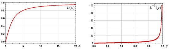
Figure 1. Graphs of the Langevin and inverse Langevin functions.

Mező and Keady [15] detail the relationship between the inverse Langevin function and a generalization of the Lambert W function. Whilst such a relationship is important, it does not directly facilitate finding approximations for the inverse Langevin function as the generalized Lambert W function does not have an explicit analytical form. The contribution of this paper is to detail a relationship between the inverse Langevin function and the r₀-r₁-Lambert W function which is a generalization of the r-Lambert W function that has been considered by Mező [16], Mező and Baricz [17], and Jamilla [18]. The derived relationship leads to new approximations for the inverse Langevin function with potentially lower relative error bounds than comparable approximations. Improved approximations, based on Schröder’s root approximations of the first kind, e.g., [19,20,21], are detailed. Several applications of the results are also detailed.

Section 2 details the definitions that underpin the paper. Section 3 details the relationship between the inverse Langevin function and the proposed r₀-r₁-Lambert W function. Section 4 details approximations for the r₀-r₁-Lambert W function and, thus, the inverse Langevin function. Section 5 details the establishment of approximations of higher accuracy through the use of Schröder’s root approximations of the first kind. Several applications of the results are detailed in Section 6. A summary of results, and conclusions, are detailed in Section 7.

2. Definitions

By utilizing the exponential function-based definition for the hyperbolic cotangent function, the following alternative definition for the Langevin function is valid:

$$\begin{array}{cc}y=L\left(x\right)=\frac{x-1+(1+x)e^{-2x}}{x(1-e^{-2x})},& x>0,y\in \left(\mathrm{0,1}\right)\end{array}.$$

(2)

It then follows that the relationship between $x$ and $y=L\left(x\right)$ is equivalently defined by either of the equations:

$$e^{-2x}=\frac{1-x(1-y)}{1+x(1-y)}$$

(3)

$$\begin{array}{cc}f\left(x,y\right)=1-\left(1-y\right)x-\left[1+\left(1+y\right)x\right]e^{-2x},& f\left(x,y\right)=0,\end{array}$$

(4)

For $x>0$, $y\in \left(\mathrm{0,1}\right)$. The graph of the function $f$ is shown in Figure 2. This function underpins a link between the inverse Langevin function and a generalization of the Lambert W function. The following definitions are fundamental to establishing the required link.

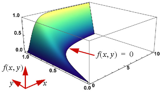
Figure 2. Graph of f(x, y).

Definition 1.

Lambert W Function.

The Lambert W function, denoted W, is the inverse of h, i.e., $h^{-1}\left(z\right)=W\left(z\right)$, where h is defined according to:

$$z=h\left(w\right)=w{e}^w.$$

(5)

For the general case, $w\in \mathit{C}$, the Lambert W function is multivalued, e.g., [22]. For the real case, $w\in (-\infty ,\infty )$, the principal branch of the Lambert W function, denoted $W_0$, is associated with the interval $w\in [-1,\infty )$ whilst the negative one branch, denoted $W_{-1}$, is associated with the interval $w\in (-\infty ,-1)$.

Definition 2.

Generalized Lambert W Function.

The generalized Lambert W function, e.g., [15], is denoted

$$W\left[\left.\begin{array}{c}{\alpha }_1,\cdots ,{\alpha }_n\\ {\beta }_1,\cdots ,{\beta }_n\end{array}\right|z\right]$$

(6)

and is the inverse of the function h which is defined according to

$$z=h\left(w\right)=e^w·\frac{(w-{\alpha }_1)\cdots (w-{\alpha }_n)}{(w-{\beta }_1)\cdots (w-{\beta }_n)}$$

(7)

For the general case $w,{\alpha }_1,\cdots ,{\alpha }_n,{\beta }_1,\cdots ,{\beta }_n\in \mathit{C}$ but often the real case is of interest.

Definition 3.

r-Lambert W Function.

The r-Lambert W function, e.g., [16,17,18], denoted $h_r^{-1}$ or $W_r$, is the inverse of $h_r$ defined according to

$$h_r\left(w\right)=rw+w{e}^w.$$

(8)

For the general case $w,r\in \mathit{C}$. A generalization of this function is the r₀-r₁-Lambert W function.

Definition 4.

r₀-r₁-Lambert W Function.

The r₀-r₁-Lambert W function, denoted $h_{r_0,r_1}^{-1}$ or $W_{r_0,r_1}$, is the inverse of $h_{r_0,r_1}$ which is defined according to:

$$h_{r_0,r_1}\left(w\right)=r_0+r_{1}w+w{e}^w.$$

(9)

For the general case $w,r_0,r_1\in \mathit{C}$. The real case is considered in this paper.

2.1. Link: Inverse Langevin Function and Generalized Lambert W Function

Manipulation of (3) (see [15] Section 2.2.1) leads to the relationship

$$L^{-1}\left(y\right)=-2W\left[\left.\begin{array}{c}\frac{2}{y+1}\\ \frac{2}{y-1}\end{array}\right|\frac{y-1}{y+1}\right]$$

(10)

which directly links the inverse Langevin function to the general Lambert W function. Whilst such a link is important, it does not directly facilitate finding approximations for the inverse Langevin function, as an explicit analytical approximation for the Lambert W function is unknown and research to develop approximations is ongoing, e.g., [23,24]. The relationship between the inverse Langevin function and the r₀-r₁-Lambert W function, which yields new approximations, is detailed below after the next subsection, which lists established approximations for the inverse Langevin function.

2.2. Published Approximations

Representative approximations for the inverse Langevin function include:

$$L_{\mathrm{0,1}}^{-1}\left(y\right)=\frac{3y}{1-y}·\left[1-\frac{24y}{25}+\frac{22y^2}{75}\right]$$

(11)

$$L_{\mathrm{0,2}}^{-1}\left(y\right)=\frac{3y}{1-y^2}·\left[1-\frac{2y^2}{5}-\frac{y^4}{15}+\frac{{2y}^6}{15}\right]$$

(12)

$$L_{\mathrm{0,3}}^{-1}\left(y\right)=3y+\frac{y^2}{5}\sin \left[\frac{7y}{2}\right]+\frac{y^3}{1-y}$$

(13)

$$L_{\mathrm{0,4}}^{-1}\left(y\right)=\frac{y\left({3-y}^2\right)}{1-y^2}-\frac{y^{10/3}}{2}+3y^5\left[y-\frac{76}{100}\right](y-1)$$

(14)

$$\begin{array}{c}{L}_{\mathrm{0,5}}^{-1}\left(y\right)=\begin{array}{cc}\frac{3y+a_2{y}^2+a_3{y}^3+a_4{y}^4}{1-y+b_2\left(y-y^2\right)+b_3\left(y^2-y^3\right)+b_4(y^3-y^4)},& \left[4/4\right] \mathrm{approx}.\end{array}\\ \begin{array}{ccc}{a}_2=-6.98408968,& a_3=5.69026957,& a_4=-1.35415696,\end{array}\\ \begin{array}{ccc}{b}_2=-1.33411915,& b_3=0.03919556,& b_4=0.64694651,\end{array}\end{array}$$

(15)

which, respectively, have been published in [5,8,11,13,14]. The relative error bounds (see definition below) that are associated with these approximations over the interval $\left[\mathrm{0,1})\right.$, respectively, are: $9.69\times {10}^{-3}$, $2.75\times {10}^{-3}$, $1.79\times {10}^{-3}$, $7.22\times {10}^{-4}$ and $1.80\times {10}^{-4}$.

2.2.1. Relative Error Bound

For an arbitrary function $f$, defined over the interval $\left[\alpha ,\beta \right]$, an approximating function $f_A$ has a relative error, at a point $x_1$, defined according to $\mathrm{re}\left(x_1\right)=1-f_A\left(x_1\right)/f\left(x_1\right)$. The relative error bound for the approximating function, over the interval $\left[\alpha ,\beta \right]$, is defined according to:

$${\mathrm{re}}_B=\max \left\{\left|\mathrm{re}\left(x_1\right)\right|: x_1\in \left[\alpha ,\beta \right]\right\}$$

(16)

In this paper, Mathematica has been used to facilitate analysis and to obtain numerical results. In general, relative error results associated with approximations have been obtained by uniformly sampling the interval $\left[\mathrm{0,1}\right]$ with 1000 points.

3. Relationship between Inverse Langevin and r₀-r₁-Lambert W Function

With the function $f$ defined according to (4), it is the case that $f\left(x,y\right)=0$ when $x=L^{-1}\left(y\right)$. The following result then holds:

Theorem 1.

Relationship: r₀-r₁-Lambert W Function and Inverse Langevin Function

With $h_{r_0,r_1}$ and $f$ defined, respectively, by (9) and (4), the general result

$$\begin{array}{cc}{h}_{r_0\left(y\right),r_1\left(y\right)}\left(w\right)=r_0\left(y\right)+r_1\left(y\right)w+w{e}^w=k_f\left(y\right)f\left[\frac{-1}{1+y}-\frac{w}{2},y\right], & y\ne -1,\end{array}$$

(17)

holds for the case of $x,y\in \mathit{R}$ when

$$\begin{array}{cc}\begin{array}{cc}\begin{array}{cc}{r}_0\left(y\right)=\frac{4e^{-2/(1+y)}}{{(1+y)}^2},& r_1\left(y\right)=\frac{(1-y)e^{-2/(1+y)}}{1+y}\end{array},& k_f\left(y\right)=\frac{2e^{-2/(1+y)}}{1+y}\end{array},& y\ne -1.\end{array}$$

(18)

It then follows that

$$\begin{array}{cc}{h}_{r_0\left(y\right),r_1\left(y\right)}\left(w\right)=\frac{4e^{-2/(1+y)}}{{(1+y)}^2}+\frac{w(1-y)e^{-2/(1+y)}}{1+y}+w{e}^w, & y\ne -1,\end{array}$$

(19)

and the inverse Langevin function can be defined according to

$$\begin{array}{cc}{L}^{-1}\left(y\right)=\frac{-1}{1+y}-\frac{h_{r_0\left(y\right),r_1\left(y\right)}^{-1}\left(0\right)}{2},& 0\le y<1.\end{array}$$

(20)

Proof of Theorem 1.

The proof is detailed in Appendix A. □

3.1. Determining Root of h

Consistent with (20), the inverse Langevin function can be defined once the appropriate root of $h_{r_0\left(y\right),r_1\left(y\right)}$ is known. It can readily be shown that

$$\begin{array}{cc}{h}_{r_0\left(y\right),r_1\left(y\right)}\left[\frac{-2}{1+y}\right]=0,& y\ne -1,\end{array}$$

(21)

which implies $h_{r_0\left(y\right),r_1\left(y\right)}^{-1}\left(0\right)=\frac{-2}{1+y}$. However, this result is associated with a branch of $h^{-1}$ which is not consistent with the validity of the relationship specified by (20). The branch of $h^{-1}$ that is required can readily be seen by considering the nature of $h$ for the case of $0<y<1$.

3.1.1. Graphs

For the case of $0\le y<1$, it is the case that $1/e<r_0\left(y\right)\le 4/e^2$ and ${0<r}_1\left(y\right)\le 1/e^2$. Graphs of $r_0\left(y\right)$ and $r_1\left(y\right)$, for the case of $y\in \left[\mathrm{0,1}\right]$, are shown in Figure 3. The graph of $h_{r_0\left(y\right),r_1\left(y\right)}\left(w\right)$ is shown in Figure 4 for two set values of $y$ to illustrate the nature of the variation of $h_{r_0\left(y\right),r_1\left(y\right)}\left(w\right)$ for set values of $y$. The variation, with $y$, of the root of $h_{r_0\left(y\right),r_1\left(y\right)}\left(w\right)$, that is to the left of $-2/(1+y)$, is shown in Figure 5.

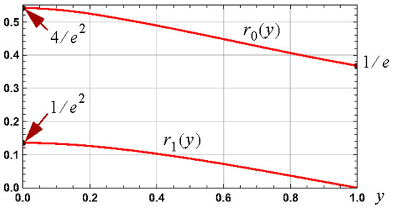
Figure 3. Graphs of $r_0\left(y\right)$ and $r_1\left(y\right)$ for the case of y ∈ (0,1).

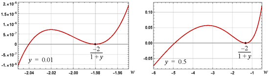
Figure 4. Graphs of $h_{r_0\left(y\right),r_1\left(y\right)}\left(w\right)$ for the set values of $y$ of 0.01 and 0.5.

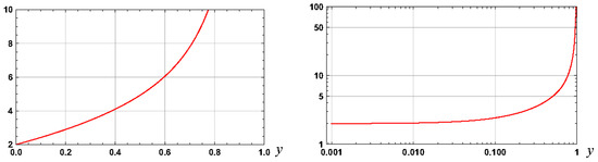
Figure 5. Graphs of $-h_{r_0\left(y\right),r_1\left(y\right)}^{-1}\left(0\right)$, $y\in \left(\mathrm{0,1}\right)$, which is the negative of the root of $h_{r_0\left(y\right),r_1\left(y\right)}\left(w\right)$ that is to the left of $-2/(1+y)$.

3.1.2. Required Branch for Root of h

The variation of $h_{r_0\left(y\right),r_1\left(y\right)}\left(w\right)$, with $w$, is illustrated in Figure 4 along with the first negative root of $w=-2/(1+y)$ as defined by (21). The required root is to the left of the local maximum of $h_{r_0\left(y\right),r_1\left(y\right)}\left(w\right)$ that is located left of the first negative root. To establish where this local maximum occurs, consider the derivative of $h_{r_0\left(y\right),r_1\left(y\right)}\left(w\right)$:

$$h_{r_0\left(y\right),r_1\left(y\right)}^{\left(1\right)}\left(w\right)=r_1\left(y\right)+\left(1+w\right)e^w.$$

(22)

The root of this function, denoted $w_m$, occurs when $\left(1+w_m\right)e^{w_m}=-r_1\left(y\right)$, or, after a change of variable $w_1=1+w_m$, where $w_1{e}^{w_1}=-e{r}_1\left(y\right)$. As ${0<r}_1\left(y\right)\le 1/e^2$, for $0\le y<1$ (see Figure 3), it is the case that

$$w_1{e}^{w_1}=\left\{\begin{array}{ll}-1/e,& y=0,r_1\left(y\right)=1/e^2\\ -e{r}_1\left(y\right),& 0<y<1, 0<r_1\left(y\right)<1/e^2\end{array}\right.$$

(23)

with solutions, consistent with the nature of the Lambert W function, e.g., [22], defined according to

$$w_1=\left\{\begin{array}{ll}-1,& y=0\\ \begin{array}{ccc}{W}_0\left[-e{r}_1\left(y\right)\right]& \mathrm{or}& W_{-1}\left[-e{r}_1\left(y\right)\right]\end{array},& 0<y<1 \end{array}\right.$$

(24)

where $W_0$ is the principal branch solution and $W_{-1}$ is the negative one branch. It is the negative one branch that provides the required solution and, thus:

$$w_m=\left\{\begin{array}{ll}-2,& y=0\\ -1+W_{-1}\left[-e{r}_1\left(y\right)\right],& 0<y<1 \end{array}\right.$$

(25)

Hence, the goal is to establish the root of $h_{r_0\left(y\right),r_1\left(y\right)}\left(w\right)$ for the case of $w\le w_m$. The nature of $z=h_{r_0\left(y\right),r_1\left(y\right)}\left(w\right)$, and its inverse $w=h_{r_0\left(y\right),r_1\left(y\right)}^{-1}\left(z\right)$, are illustrated in Figure 6 for the case of $w\le w_m$ and a fixed value of $y$.

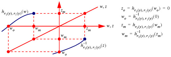
Figure 6. Illustration of the functions $z=h_{r_0\left(y\right),r_1\left(y\right)}\left(w\right)$ and $w=h_{r_0\left(y\right),r_1\left(y\right)}^{-1}\left(z\right)$ for $y$ fixed and $w\le w_m$.

4. Approximations for Inverse Langevin Function

Consistent with Theorem 1, an approximation to $h_{r_0\left(y\right),r_1\left(y\right)}^{-1}\left(0\right)$, for $0\le y<1$, leads to an approximation for the inverse Langevin function. To establish approximations for $h_{r_0\left(y\right),r_1\left(y\right)}^{-1}\left(0\right)$, first, consider the following two restricted domain approximations which arise from the analysis detailed in Appendix B:

$$\begin{array}{ll}{h}_{r_0\left(y\right),r_1\left(y\right)}^{-1}\left(0\right)\approx -2-4y,& 0<y\ll 1,\\ h_{r_0\left(y\right),r_1\left(y\right)}^{-1}\left(0\right)\approx \frac{-2}{1-y}, & y=1-\mathsf{\Delta },0<∆\ll 1.\end{array}$$

(26)

These approximations are consistent with the first order approximation:

$$\begin{array}{cc}{h}_{{1,r}_0\left(y\right),r_1\left(y\right)}^{-1}\left(0\right)=\frac{-2}{1-y}-2y=\frac{-2}{1-y}·\left[1+y-y^2\right],& 0\le y<1,\end{array}$$

(27)

Consistency arises, first, by noting $-2/\left(1-y\right)\approx -2(1+y)$, $0<y\ll 1$, and thus, the approximation for $y\to 0$ is $-2-4y$ as required. Second, for the case of $y=1-\mathsf{\Delta }$, $0<\mathsf{\Delta }\ll 1$, the approximation approaches $-2/\left(1-y\right)$ as required. A measure of the error in this approximation is shown in Figure 7 and the relative error bound associated with the interval $\left(\mathrm{0,1}\right)$ is $4.45\times {10}^{-2}$.

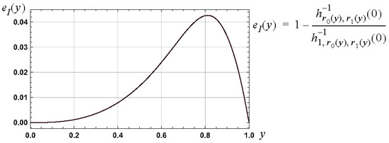
Figure 7. Graph, over the interval $y\in \left(\mathrm{0,1}\right)$, of a measure of the relative error, $e_I$, in the approximation $h_{{1,r}_0\left(y\right),r_1\left(y\right)}^{-1}\left(0\right)$, as defined by (27), to $h_{r_0\left(y\right),r_1\left(y\right)}^{-1}\left(0\right)$.

The approximation defined by (27) and the relative error measure $e_I$ shown in Figure 7 are consistent with

$$h_{r_0\left(y\right),r_1\left(y\right)}^{-1}\left(0\right)=h_{{1,r}_0\left(y\right),r_1\left(y\right)}^{-1}\left(0\right)·\left[1-e_I\left(y\right)\right],$$

(28)

and this relationship provides a useful basis for establishing better approximations. Improved approximations include:

$$\begin{array}{c}{h}_{{2,r}_0\left(y\right),r_1\left(y\right)}^{-1}\left(0\right)=\frac{-2}{1-y}·\left[1+c_{21}\sin \left(\pi y\right)+c_{22}\sin \left(\pi y^2\right)\right] \\ \begin{array}{cc}{c}_{21}=\frac{281}{1000},& c_{22}=\frac{-65}{1000}\end{array}\end{array}$$

(29)

$${ h}_{{3,r}_0\left(y\right),r_1\left(y\right)}^{-1}\left(0\right)=\frac{-2}{1-y}·\left[1+y-y^2\right]+y^{7/2}=\frac{-2}{1-y}·\left[1+y-y^2-\frac{y^{7/2}}{2}+\frac{y^{9/2}}{2}\right]$$

(30)

$$\begin{array}{cc}\hfill h_{{4,r}_0\left(y\right),r_1\left(y\right)}^{-1}\left(0\right)& =\frac{-2}{1-y}·\left[1+y-y^2\right]·\left[1-\frac{y^4(1-y)}{2}\right]\hfill \\ & =\frac{-2}{1-y}·\left[1+y-y^2-\frac{y^4}{2}+y^6-\frac{y^7}{2}\right]\hfill \end{array}$$

(31)

$$\begin{array}{c}{h}_{{5,r}_0\left(y\right),r_1\left(y\right)}^{-1}\left(0\right)=\frac{-2}{1-y}·\left[1+y-y^2-\frac{y^{7/2}}{2}+\frac{y^{9/2}}{2}\right]+c_{51}{y}^5\left(1-y\right)(y-y_o)e^{-3{(y-y_o)}^2} \\ \begin{array}{cc}{c}_{51}=\frac{1133}{200},& y_o=\frac{2212}{3125}\end{array}\end{array}$$

(32)

$$\begin{array}{cc}\hfill h_{{6,r}_0\left(y\right),r_1\left(y\right)}^{-1}\left(0\right)=& \frac{-2}{1-y}·\left[1+y-y^2-\frac{y^4}{2}+y^6-\frac{y^7}{2}\right]\hfill \\ & \left[1+{\alpha }_0{y}^2{(1-y)}^2\left[1+{\alpha }_2{y}^2+{\alpha }_3{y}^3+{\alpha }_4{y}^4+{\alpha }_5{y}^5+{\alpha }_7{y}^7+{\alpha }_8{y}^8\right]\right]\hfill \\ & {\alpha }_0=\frac{-5813}{\mathrm{1,000,000}},{\alpha }_2=\frac{3349}{10},{\alpha }_3=\frac{-23467}{10},{\alpha }_4=6526,\hfill \\ & {\alpha }_5=-7920,{\alpha }_7=8222,{\alpha }_8=-4799.\hfill \end{array}$$

(33)

Graphs of the magnitude of the relative errors in these approximations are shown in Figure 8. The respective relative error bounds associated with these approximations, and for the interval $\left(\mathrm{0,1}\right)$, are: $4.66\times {10}^{-3}$, $3.71\times {10}^{-3}$, $2.13\times {10}^{-3}$, $2.33\times {10}^{-4}$ and $4.58\times {10}^{-5}$.

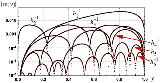
Figure 8. Graphs of the magnitude of the relative error in approximations to $h_{r_0\left(y\right),r_1\left(y\right)}^{-1}\left(0\right)$ as defined by (27) and (29) to (33).

4.1. Associated Langevin Approximations

Given the relationship $L^{-1}\left(y\right)=\frac{-1}{1+y}-\frac{h_{r_0\left(y\right),r_1\left(y\right)}^{-1}\left(0\right)}{2}$, as stated in Theorem 1, the above approximations for $h_{r_0\left(y\right),r_1\left(y\right)}^{-1}\left(0\right)$, as specified by (27) and (28) to (33), lead, respectively, to the following approximations for the inverse Langevin function:

$$L_1^{-1}\left(y\right)=\frac{3y}{1-y^2}·\left[1-\frac{y^2}{3}\right]$$

(34)

$$\begin{array}{c}{L}_2^{-1}\left(y\right)=\frac{2y}{1-y^2}+\frac{d_{21}\sin \left(\pi y\right)+d_{22}\sin \left(\pi y^2\right)}{1-y}\\ \begin{array}{cc}{d}_{21}=\frac{301}{1000},& d_{22}=\frac{-92}{1000}\end{array}.\end{array}$$

(35)

$$L_3^{-1}\left(y\right)=\frac{3y}{1-y^2}·\left[1-\frac{y^2}{3}-\frac{y^{5/2}}{6}+\frac{y^{9/2}}{6}\right]$$

(36)

$$L_4^{-1}\left(y\right)=\frac{3y}{1-y^2}·\left[1-\frac{y^2}{3}-\frac{y^3}{6}-\frac{y^4}{6}+\frac{y^5}{3}+\frac{y^6}{6}-\frac{y^7}{6}\right]$$

(37)

$$L_5^{-1}\left(y\right)=\frac{3y}{1-y^2}·\left[1-\frac{y^2}{3}-\frac{y^{5/2}}{6}+\frac{y^{9/2}}{6}\right]-\frac{c_{51}{y}^5\left(1-y\right)(y-y_o)}{2}·e^{-3{(y-y_o)}^2}$$

(38)

$$L_6^{-1}\left(y\right)=\frac{3y}{1-y^2}·\left[\begin{array}{l}1-\frac{y^2}{3}-\frac{y^3}{6}-\frac{y^4}{6}+\frac{y^5}{3}+\frac{y^6}{6}-\frac{y^7}{6}+\\ \frac{{\alpha }_{0}y{(1-y^2)}^2}{3}·\left[1-y^2+y^3-\frac{3y^4}{2}+\frac{3y^5}{2}-\frac{y^6}{2}\right]·\\ \left[1+{\alpha }_2{y}^2+{\alpha }_3{y}^3+{\alpha }_4{y}^4+{\alpha }_5{y}^5+{\alpha }_7{y}^7+{\alpha }_8{y}^8\right]\end{array}\right]$$

(39)

Graphs of the magnitude of the relative errors in these approximations are shown in Figure 9. The relative error bounds associated with these approximations, and for the interval $\left(\mathrm{0,1}\right)$, respectively, are: $4.94\times {10}^{-2}$, $1.83\times {10}^{-2}$, $4.37\times {10}^{-3}$, $2.44\times {10}^{-3}$, $2.58\times {10}^{-4}$ and $4.85\times {10}^{-5}$.

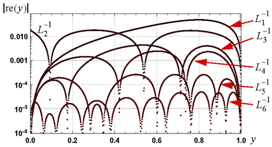
Figure 9. Graphs of the magnitude of the relative error in approximations to $L^{-1}\left(y\right)$ as defined by (34) to (39).

Notes

The coefficients utilized in the approximations $h_{{2,r}_0\left(y\right),r_1\left(y\right)}^{-1}$ and $L_2^{-1}$ are different and have been chosen to minimize their respective relative error bounds over the interval $\left[\mathrm{0,1}\right)$.

The fourth approximation, as given by (37), has a relative error bound of $2.44\times {10}^{-3}$ over the interval $\left[\mathrm{0,1}\right).$ and is similar in form to that proposed by Kröger [8] and stated in (12). The proposed approximation includes an order seven (rather than six) polynomial and achieves a slightly lower relative error bound.

The fifth (38) and sixth (39) approximations achieve lower relative error bounds, respectively, than the published approximations provided by Nguessong [5] and Marchi [13] and which are stated in (14) and (15).

The proposed approximations complement the list of published approximations for the inverse Langevin function and with relative error bounds consistent with, or lower than, comparable published approximations. Additional approximations remain to be proposed.

5. Schröder Based Higher Order Approximations

The following general approximations for an inverse function arise from the Schröder root approximation of the first kind, e.g., [25] (Equation (21)), [19] (Equation (17)), [20] (Section 3) and [21]:

Theorem 2.

Schröder Based Approximations for an Inverse Function

Consider a real function $f$ that is differentiable up to at least order $n$ and is also strictly monotonic in an interval around a point $x_0$ which includes the root $x_o$ of $g\left(x\right)=f\left(x\right)-y_o$ that is close to $x_0$ . A $n\mathrm{t}\mathrm{h}$ order Taylor series for $g^{-1}$ , based on the point $\left(y_0,x_0\right)$ , $y_0=f\left(x_0\right)-y_o$ , yields the $n\mathrm{t}\mathrm{h}$ order Schröder approximation for $x_o=f^{-1}\left(y_o\right)$ , denoted $x_n$ , and defined according to

$$x_n=x_0+\sum _{k=1}^n\frac{{\left(-1\right)}^k{\left[f\left(x_0\right)-y_o\right]}^k}{k!}·D^{\left(k\right)}\left[f^{-1}\left[f\left(x_0\right)\right]\right], n\in \left\{\mathrm{1,2},\cdots \right\},$$

(40)

where $D^{\left(k\right)}$ is the operator denoting $k\mathrm{th}$ order differentiation. An explicit form is

$$\begin{array}{l}{{\mathrm{x}}_n=x}_0-\frac{f\left(x_0\right)-y_o}{f^{\left(1\right)}\left(x_0\right)}-\frac{{\left[f\left(x_0\right)-y_o\right]}^2{f}^{\left(2\right)}\left(x_0\right) }{{2\left[f^{\left(1\right)}\left(x_0\right)\right]}^3}-\frac{{\left[f\left(x_0\right)-y_o\right]}^3{f}^{\left(3\right)}\left(x_0\right) }{{6\left[f^{\left(1\right)}\left(x_0\right)\right]}^4}·\left[-1+\frac{3{\left[f^{\left(2\right)}\left(x_0\right)\right]}^2 }{f^{\left(1\right)}\left(x_0\right)f^{\left(3\right)}\left(x_0\right)}\right]-\\ \frac{{\left[f\left(x_0\right)-y_o\right]}^4{f}^{\left(4\right)}\left(x_0\right) }{{24\left[f^{\left(1\right)}\left(x_0\right)\right]}^5}·\left[1-\frac{10f^{\left(2\right)}\left(x_0\right)f^{\left(3\right)}\left(x_0\right) }{f^{\left(1\right)}\left(x_0\right)f^{\left(4\right)}\left(x_0\right)}+\frac{15{\left[f^{\left(2\right)}\left(x_0\right)\right]}^3 }{{\left[f^{\left(1\right)}\left(x_0\right)\right]}^2{f}^{\left(4\right)}\left(x_0\right)}\right]-\\ \begin{array}{l}\frac{{\left[f\left(x_0\right)-y_o\right]}^5{f}^{\left(5\right)}\left(x_0\right) }{{120\left[f^{\left(1\right)}\left(x_0\right)\right]}^6}·\left[\begin{array}{c}-1+\frac{15f^{\left(2\right)}\left(x_0\right)f^{\left(4\right)}\left(x_0\right) }{f^{\left(1\right)}\left(x_0\right)f^{\left(5\right)}\left(x_0\right)}+\frac{10{\left[f^{\left(3\right)}\left(x_0\right)\right]}^2 }{f^{\left(1\right)}\left(x_0\right)f^{\left(5\right)}\left(x_0\right)}-\\ \frac{105{\left[f^{\left(2\right)}\left(x_0\right)\right]}^2{f}^{\left(3\right)}\left(x_0\right) }{{\left[f^{\left(1\right)}\left(x_0\right)\right]}^2{f}^{\left(5\right)}\left(x_0\right)}+\frac{105{\left[f^{\left(2\right)}\left(x_0\right)\right]}^4 }{{\left[f^{\left(1\right)}\left(x_0\right)\right]}^3{f}^{\left(5\right)}\left(x_0\right)}\end{array}\right]-\\ \frac{{\left[f\left(x_0\right)-y_o\right]}^6{f}^{\left(6\right)}\left(x_0\right) }{{720\left[f^{\left(1\right)}\left(x_0\right)\right]}^7}·\left[\begin{array}{c}1-\frac{21f^{\left(2\right)}\left(x_0\right)f^{\left(5\right)}\left(x_0\right) }{f^{\left(1\right)}\left(x_0\right)f^{\left(6\right)}\left(x_0\right)}-\frac{35f^{\left(3\right)}\left(x_0\right)f^{\left(4\right)}\left(x_0\right) }{f^{\left(1\right)}\left(x_0\right)f^{\left(6\right)}\left(x_0\right)}+\frac{210{\left[f^{\left(2\right)}\left(x_0\right)\right]}^2{f}^{\left(4\right)}\left(x_0\right) }{{\left[f^{\left(1\right)}\left(x_0\right)\right]}^2{f}^{\left(6\right)}\left(x_0\right)}+\\ \frac{280f^{\left(2\right)}\left(x_0\right){\left[f^{\left(3\right)}\left(x_0\right)\right]}^2 }{{\left[f^{\left(1\right)}\left(x_0\right)\right]}^2{f}^{\left(6\right)}\left(x_0\right)}-\frac{1260{\left[f^{\left(2\right)}\left(x_0\right)\right]}^3{f}^{\left(3\right)}\left(x_0\right) }{{\left[f^{\left(1\right)}\left(x_0\right)\right]}^3{f}^{\left(6\right)}\left(x_0\right)}+\frac{945{\left[f^{\left(2\right)}\left(x_0\right)\right]}^5 }{{\left[f^{\left(1\right)}\left(x_0\right)\right]}^4{f}^{\left(6\right)}\left(x_0\right)}\end{array}\right]-\\ \cdots +\frac{{{\left(-1\right)}^n\left[f\left(x_0\right)-y_o\right]}^n}{n!}·D^{\left(\mathrm{n}\right)}\left[f^{-1}\left[f\left(x_0\right)\right]\right]\end{array}\end{array}$$

(41)

Proof of Theorem 2.

This result arises from a Taylor series approximation for $g^{-1}$ at the point $\left(y_0,x_0\right)$ and the inverse function theorem. See, for example, [21]. □

5.1. First, Second and Third Order Approximations for h⁻¹(0)

Consider $h_{r_0\left(y\right),r_1\left(y\right)}\left(w\right)=r_0\left(y\right)+r_1\left(y\right)w+w{e}^w$, with $r_0$ and $r_1$ as defined in (18), and an initial approximation for $h_{r_0\left(y\right),r_1\left(y\right)}^{-1}\left(0\right)$ being denoted $h_0^{-1}\left(0\right)$ where the argument of $y$ is implicit and assumed to be on the interval $\left[\mathrm{0,1}\right)$. It then follows that the first, second, and third order Schröder based approximations for $h_{r_0\left(y\right),r_1\left(y\right)}^{-1}\left(0\right)$, denoted, respectively, $h_1^{-1}\left(0\right)$, $h_2^{-1}\left(0\right)$, and $h_3^{-1}\left(0\right)$ are:

$$h_1^{-1}\left(0\right)={\left.\frac{-4+{\left(1+y\right)}^2{w}^2\exp \left[w+\frac{2}{1+y}\right]}{1-y^2+{\left(1+y\right)}^2(1+w)\exp \left[w+\frac{2}{1+y}\right]}\right|}_{{w=h}_0^{-1}\left(0\right)}$$

(42)

$$\begin{array}{l}{h}_2^{-1}\left(0\right)=\frac{-4+{\left(1+y\right)}^2{w}^2\exp \left[w+\frac{2}{1+y}\right]}{1-y^2+{\left(1+y\right)}^2(1+w)\exp \left[w+\frac{2}{1+y}\right]}-\\ {\left. \frac{{\left[4+\left(1-y^2\right)w+{\left(1+y\right)}^{2}w\exp \left[w+\frac{2}{1+y}\right]\right]}^2(2+w)\exp \left[w+\frac{2}{1+y}\right]}{2(1+y){\left[1-y+(1+y)(1+w)\exp \left[w+\frac{2}{1+y}\right]\right]}^3}\right|}_{{w=h}_0^{-1}\left(0\right)}\end{array}$$

(43)

$$\begin{array}{l}{h}_3^{-1}\left(0\right)=h_2^{-1}\left(0\right)-\\ {\left. \begin{array}{c}{\left[4+\left(1-y^2\right)w+{\left(1+y\right)}^{2}w\exp \left[w+\frac{2}{1+y}\right]\right]}^3\exp \left[w+\frac{2}{1+y}\right]·\\ \frac{\left[-(1-y)(3+w)+\left(1+y\right)(9+8w+2w^2)\exp \left[w+\frac{2}{1+y}\right]\right]}{6{(1+y)}^2{\left[1-y+(1+y)(1+w)\exp \left[w+\frac{2}{1+y}\right]\right]}^5}\end{array}\right|}_{{w=h}_0^{-1}\left(0\right)}\end{array}$$

(44)

The proofs for these results are detailed in Appendix C.

Results

The relative error bounds associated with the above approximations, and based on $h_0^{-1}\left(0\right)$ as specified by (27) and (29) to (33), are detailed in Table 1. Specific cases are detailed below.

5.2. First Order Approximations: Explicit Cases

The general first order approximation form specified by (42) leads to the approximations detailed below which are valid for $y\in \left[\mathrm{0,1}\right)$. The associated approximations for the inverse Langevin function can then be defined consistent with Theorem 1.

5.2.1. Case 1

With the initial approximation $h_{{1,r}_0\left(y\right),r_1\left(y\right)}^{-1}\left(0\right)$ specified by (27), it follows that

$$h_1^{-1}\left(0\right)=\frac{-4{\left(1-y\right)}^2+{4\left(1+2y-y^3\right)}^2\exp \left[\frac{-6y}{1-y^2}·\left[1-\frac{y^2}{3}\right]\right]}{(1+y){\left(1-y\right)}^3-(1-y^2)(1+4y+y^2-{2y}^3)\exp \left[\frac{-6y}{1-y^2}·\left[1-\frac{y^2}{3}\right]\right]}$$

(45)

which has a relative error bound of $2.69\times {10}^{-4}$. The relative error bound in the associated approximation for the inverse Langevin function is $3.36\times {10}^{-4}$.

5.2.2. Case 2

With the approximation $h_{{3,r}_0\left(y\right),r_1\left(y\right)}^{-1}\left(0\right)$ defined by (30), it follows, that

$$\begin{array}{cc}\hfill h_1^{-1}\left(0\right)=& \frac{-4{\left(1-y\right)}^2+{\left(1+y\right)}^2{\left[-2-2y+2y^2+y^{7/2}-y^{9/2}\right]}^2\mathrm{e}\mathrm{x}\mathrm{p}\left[p_E\right(y\left)\right]}{{\left(1-y\right)}^3\left(1+y\right)-(1-y){\left(1+y\right)}^2\left[1+3y-2y^2-y^{7/2}+y^{9/2}\right]\mathrm{e}\mathrm{x}\mathrm{p}\left[p_E\right(y\left)\right]}\hfill \\ & p_E\left(y\right)=\frac{-6y}{1-y^2}·\left[1-\frac{y^2}{3}-\frac{y^{5/2}}{6}+\frac{y^{9/2}}{6}\right]\hfill \end{array}$$

(46)

which has a relative error bound of $8.52\times {10}^{-6}$. The relative error bound in the associated approximation for the inverse Langevin function is $1.17\times {10}^{-5}$.

5.2.3. Case 3

With the approximation $h_{{4,r}_0\left(y\right),r_1\left(y\right)}^{-1}\left(0\right)$ defined by (31), it follows that

$$\begin{array}{cc}\hfill h_1^{-1}\left(0\right)=& \frac{-4{\left(1-y\right)}^2+{4\left(1+y\right)}^2{\left[1+y-y^2-\frac{y^4}{2}+y^6-\frac{y^7}{2}\right]}^2\mathrm{e}\mathrm{x}\mathrm{p}\left[p_E\right(y\left)\right]}{{\left(1-y\right)}^3\left(1+y\right)-(1-y){\left(1+y\right)}^2\left[1+3y-2y^2-y^4+{2y}^6-y^7\right]\mathrm{e}\mathrm{x}\mathrm{p}\left[p_E\right(y\left)\right]}\hfill \\ & p_E\left(y\right)=\frac{-6y}{1-y^2}·\left[1-\frac{y^2}{3}-\frac{y^3}{6}-\frac{y^4}{6}+\frac{y^5}{3}+\frac{y^6}{6}-\frac{y^7}{6}\right]\hfill \end{array}$$

(47)

which has a relative error bound of $1.92\times {10}^{-6}$. The relative error bound in the associated approximation for the inverse Langevin function is $2.66\times {10}^{-6}$.

5.2.4. Case 4

With the approximation $h_{{6,r}_0\left(y\right),r_1\left(y\right)}^{-1}\left(0\right)$ defined by (33), it follows that

$$\begin{array}{c}{ h}_1^{-1}\left(0\right)=\frac{-4{\left(1-y\right)}^2+{4\left(1+y\right)}^2{\left[1+y-y^2-\frac{y^4}{2}+y^6-\frac{y^7}{2}\right]}^2{p}^2\left(y\right)\mathrm{e}\mathrm{x}\mathrm{p}\left[p_E\right(y\left)\right]}{{\left(1-y\right)}^3\left(1+y\right)+(1-y){\left(1+y\right)}^2\left[1-y-2\left[1+y-y^2-\frac{y^4}{2}+y^6-\frac{y^7}{2}\right]p\left(y\right)\right]\mathrm{e}\mathrm{x}\mathrm{p}\left[p_E\right(y\left)\right]}\\ \end{array}$$

(48)

where

$$p\left(y\right)=1+{\alpha }_0{y}^2{(1-y)}^2\left[1+{\alpha }_2{y}^2+{\alpha }_3{y}^3+{\alpha }_4{y}^4+{\alpha }_5{y}^5+{\alpha }_7{y}^7+{\alpha }_8{y}^8\right]$$

(49)

$$p_E\left(y\right)=\frac{-6y}{1-y^2}·\left[\begin{array}{l}1-\frac{y^2}{3}-\frac{y^3}{6}-\frac{y^4}{6}+\frac{y^5}{3}+\frac{y^6}{6}-\frac{y^7}{6}+\\ \frac{{\alpha }_{0}y{(1-y^2)}^2}{3}·\left[1-y^2+y^3-\frac{3y^4}{2}+\frac{3y^5}{2}-\frac{y^6}{2}\right]·\\ \left[1+{\alpha }_2{y}^2+{\alpha }_3{y}^3+{\alpha }_4{y}^4+{\alpha }_5{y}^5+{\alpha }_7{y}^7+{\alpha }_8{y}^8\right]\end{array}\right]$$

(50)

This approximation has a relative error bound of $4.07\times {10}^{-10}$. The relative error bound in the associated approximation for the inverse Langevin function is $6.27\times {10}^{-10}$.

5.3. Second Order Approximations

With the approximation $h_{{4,r}_0\left(y\right),r_1\left(y\right)}^{-1}\left(0\right)$ defined by (31), it follows, from (43), that:

$$\begin{array}{cc}\hfill h_2^{-1}\left(0\right)=& h_1^{-1}\left(0\right)+\hfill \\ & 8y{\left[\begin{array}{l}-{\left(1-y\right)}^3\left[1-y^2-y^3-\frac{y^4}{2}+\frac{y^5}{2}+\frac{y^6}{2}\right]+\\ {\left(1+y\right)}^3\left[1-y^2+y^3-\frac{{3y}^4}{2}+\frac{{3y}^5}{2}-\frac{y^6}{2}\right]\mathrm{e}\mathrm{x}\mathrm{p}\left[p_E\right(y\left)\right]\end{array}\right]}^2·\hfill \\ & \frac{\left[1-\frac{y^2}{2}-\frac{y^3}{4}+\frac{y^5}{2}-\frac{y^6}{4}\right]\mathrm{e}\mathrm{x}\mathrm{p}\left[p_E\right(y\left)\right]}{\left(1+y\right){\left[{\left(1-y\right)}^2-(1+y)\left[1+3y-2y^2-y^4+{2y}^6-y^7\right]\mathrm{e}\mathrm{x}\mathrm{p}\left[p_E\right(y\left)\right]\right]}^3}\hfill \end{array}$$

(51)

where $h_1^{-1}\left(0\right)$ and $p_E\left(y\right)$ are defined by (47). The relative error bound for this approximation is $9.12\times {10}^{-9}$. The relative error bound in the associated approximation for the inverse Langevin function is $1.16\times {10}^{-8}$.

5.4. Direct First Order Schröder Approximation to Inverse Langevin Function

Consider the first order Schröder approximation to the inverse Langevin function, based on an initial approximation denoted $L_0^{-1}$, and defined by

$$L_1^{-1}\left(y\right)=x-{\frac{L\left(x\right)-y}{L^{\left(1\right)}\left(x\right)}⌋}_{x=L_0^{-1}\left(y\right)}$$

(52)

The nature of $L_1^{-1}$ depends on the form assumed for the Langevin function. For the case of $L$ defined according to $L\left(x\right)=\coth \left(x\right)-1/x$, it follows that:

$$L_1^{-1}\left(y\right)={\frac{x^3-x\sinh \left(x\right)⌈2\sinh (x)-x\cosh \left(x\right)+xy\sinh \left(x\right)⌉}{x^2-{\sinh \left(x\right)}^2}⌋}_{x=L_0^{-1}\left(y\right)}$$

(53)

For the case of $L$ defined according to (3), it follows that:

$$L_1^{-1}\left(y\right)={\frac{x\left[2-x+xy\right]-2x\left[2+2x^2+xy\right]e^{-2x}+x[2+x+xy]e^{-4x}}{1-2\left[1+2x^2\right]e^{-2x}+e^{-4x}}⌋}_{x=L_0^{-1}\left(y\right)}$$

(54)

Comparison

The approximations defined by (53) and (54) can be contrasted with approximating the inverse Langevin function according to the relationship stated in Theorem 1, i.e.,

$$L^{-1}\left(y\right)\approx \frac{-1}{1+y}-\frac{h_1^{-1}\left(0\right)}{2}$$

(55)

where $h_1^{-1}\left(0\right)$ is the first order approximation defined according to (42). To compare the approximations defined by (54) and (55), consider the initial approximations

$$L_0^{-1}\left(y\right)=\frac{3y}{1-y^2}·\left[1-\frac{2y^2}{5}-\frac{y^4}{15}+\frac{{2y}^6}{15}\right]$$

(56)

$$h_0^{-1}\left(0\right)=\frac{-2}{1-y}·\left[1+y-y^2-\frac{y^4}{2}+y^6-\frac{y^7}{2}\right]$$

(57)

The first was proposed by Kröger [8] (stated above in (12)) and has a relative error bound of $2.75\times {10}^{-3}$. The second approximation is specified in (31) and has a relative error bound of $2.13\times {10}^{-3}$. Use of (56) in (54) yields the approximation

$$\begin{array}{l}\begin{array}{l}{ L}_1^{-1}\left(y\right)={-p}_E\left(y\right)\\ \begin{array}{c}\begin{array}{c} \frac{\left[\begin{array}{c}\begin{array}{c}\begin{array}{c}{\left(1-y\right)}^2\left[1+\frac{y}{2}-\frac{y^2}{2}+\frac{{3y}^3}{5}+\frac{{3y}^4}{5}+\frac{y^5}{10}+\frac{y^6}{10}-\frac{y^7}{5}-\frac{y^8}{5}\right]+ \\ {\left(1+y\right)}^2\left[1-\frac{y}{2}-\frac{y^2}{2}-\frac{{3y}^3}{5}+\frac{{3y}^4}{5}-\frac{y^5}{10}+\frac{y^6}{10}+\frac{y^7}{5}-\frac{y^8}{5}\right]e^{2p_E\left(y\right)}- \end{array}\\ 2\left[1+\frac{{17y}^2}{2}-\frac{{83y}^4}{10}+\frac{{37y}^6}{50}+\frac{159y^8}{50}-\frac{28y^{10}}{25}-\frac{{4y}^{12}}{25}+\frac{{4y}^{14}}{25}\right]e^{p_E\left(y\right)}\end{array}\end{array}\right]}{{\left(1-y^2\right)}^2\left[1+e^{2p_E\left(y\right)}\right]-2\left[1+{16y}^2-\frac{{67y}^4}{5}+\frac{{12y}^6}{25}+\frac{144y^8}{25}-\frac{46y^{10}}{25}-\frac{{8y}^{12}}{25}+\frac{{8y}^{14}}{25}\right]e^{{2p}_E\left(y\right)}}\end{array}\end{array}\end{array}\\ { p}_E\left(y\right)=\frac{-6y}{1-y^2}·\left[1-\frac{{2y}^2}{5}-\frac{y^4}{15}+\frac{2y^6}{15}\right] \end{array}$$

(58)

with a relative error bound of $7.34\times {10}^{-6}$. In contrast, the use of (57) in (42), and then (55), leads to the approximation specified in (47), i.e.,

$$\begin{array}{cc}\hfill h_1^{-1}\left(0\right)=& \frac{-4{\left(1-y\right)}^2+{4\left(1+y\right)}^2{\left[1+y-y^2-\frac{y^4}{2}+y^6-\frac{y^7}{2}\right]}^2\mathrm{e}\mathrm{x}\mathrm{p}[p_E(y)]}{{\left(1-y\right)}^3\left(1+y\right)-(1-y){\left(1+y\right)}^2\left[1+3y-2y^2-y^4+{2y}^6-y^7\right]\mathrm{e}\mathrm{x}\mathrm{p}[p_E(y)]}\hfill \\ & p_E\left(y\right)=\frac{-6y}{1-y^2}·\left[1-\frac{y^2}{3}-\frac{y^3}{6}-\frac{y^4}{6}+\frac{y^5}{3}+\frac{y^6}{6}-\frac{y^7}{6}\right] \hfill \end{array}$$

(59)

which has a relative error bound of $1.92\times {10}^{-6}$. The associated approximation for $L^{-1}\left(y\right)$ is

$$L_1^{-1}\left(y\right)=\frac{-1}{1+y}-\frac{h_1^{-1}\left(0\right)}{2}$$

(60)

and has a relative error bound of $2.66\times {10}^{-6}$.

Clearly, (59) and (60) have a simpler form than (58) and yield an approximation for $L^{-1}\left(y\right)$ with a lower relative error bound. This, in part, is the rationale for the use of the link between the inverse Langevin function and the r₀-r₁-Lambert W function.

6. Applications

6.1. Limit Approximations

The approximations detailed in (26) lead to the following approximations for the inverse Langevin function after using the relationship defined in Theorem 1:

$$\begin{array}{ll}{L}^{-1}\left(y\right)\approx \frac{3y}{1+y}·\left[1+\frac{2y}{3}\right],& 0<y\ll 1,\\ L^{-1}\left(y\right)\approx \frac{2y}{1-y^2}, & y=1-\mathsf{\Delta },0<∆\ll 1.\end{array}$$

(61)

These approximations can be contrasted with established approximations. First, a Taylor series approximation for the inverse Langevin function, e.g., [4], is

$$L^{-1}\left(y\right)\approx 3y+\frac{9y^3}{5}+\frac{{297y}^5}{175}+\frac{1539y^7}{875}+\cdots$$

(62)

Second, a first order approximation for the case of $y=1-\mathsf{\Delta }$, $0<∆\ll 1$, is $L^{-1}\left(y\right)\approx 1/(1-y)$ (see Appendix B of [8]). The graphs of the relative errors associated with these approximations are shown in Figure 10. It is clear from these graphs that the approximations defined in (61) are inferior to established approximations for arguments close to zero or close to one. However, they serve as a useful basis for establishing approximations with low relative error bounds over the interval $\left(\mathrm{0,1}\right)$ for $h^{-1}$ and, hence, $L^{-1}$, as summarized in Table 2.

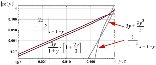
Figure 10. Graph of the relative errors in approximations to the inverse Langevin function for the cases of $0<y\ll 1$ and $y=1-\mathsf{\Delta },$ $0<∆\ll 1.$

6.2. Integral Results

As $\underset{0}{\overset{x}{\int }}L\left(\lambda \right)d\lambda =\ln \left[\sinh \left(x\right)\right]-\ln \left(x\right)$, the general integral result

$$\underset{y_1}{\overset{y}{\int }}{f}^{-1}\left(\lambda \right)d\lambda =y{f}^{-1}\left(y\right)-y_1{f}^{-1}\left(y_1\right)-\underset{f^{-1}\left(y_1\right)}{\overset{f^{-1}\left(y\right)}{\int }}f\left(\lambda \right)d\lambda$$

(63)

assuming $f^{-1}$ and $f$ are well defined, yields

$$\begin{array}{cc}\underset{0}{\overset{y}{\int }}{L}^{-1}\left(\lambda \right)d\lambda =y{L}^{-1}\left(y\right)+\ln \left[L^{-1}\left(y\right)\right]-\ln \left[\sinh \left[L^{-1}\left(y\right)\right]\right],& y\in \left(\mathrm{0,1}\right).\end{array}$$

(64)

The proposed approximations can be utilized to establish approximations for the integral of the inverse Langevin function. For example, use of the approximations specified by (36) and (37), in (64), yield approximations for the inverse Langevin function with the respective relative error bounds of $1.40\times {10}^{-5}$ and $3.91\times {10}^{-6}$. The latter approximation is:

$$\begin{array}{cc}\hfill \underset{0}{\overset{y}{\int }}{L}^{-1}\left(\lambda \right)d\lambda & \approx \frac{3y^2}{1-y^2}·\left[1-\frac{y^2}{3}-\frac{y^3}{6}-\frac{y^4}{6}+\frac{y^5}{3}+\frac{y^6}{6}-\frac{y^7}{6}\right]+\hfill \\ & \ln \left[\frac{3y}{1-y^2}·\left[1-\frac{y^2}{3}-\frac{y^3}{6}-\frac{y^4}{6}+\frac{y^5}{3}+\frac{y^6}{6}-\frac{y^7}{6}\right]\right]-\hfill \\ & \begin{array}{cc}\ln \left[\sinh \left[\frac{3y}{1-y^2}·\left[1-\frac{y^2}{3}-\frac{y^3}{6}-\frac{y^4}{6}+\frac{y^5}{3}+\frac{y^6}{6}-\frac{y^7}{6}\right]\right]\right],& y\in \left(\mathrm{0,1}\right).\end{array}\hfill \end{array}$$

(65)

6.3. Roots of $\alpha +\beta w+w{e}^w$

Consistent with (21) and Theorem 1, the roots of $h_{r_0\left(y\right),r_1\left(y\right)}\left(w\right)=r_0\left(y\right)+r_1\left(y\right)w+w{e}^w$, $0<y<1$ are $\frac{-2}{1+y}$ and $\frac{-2}{1+y}-2L^{-1}\left(y\right)$. A desirable extension to these results would be a specification of the roots of

$$h_{\alpha ,\beta }\left(w\right)=\alpha +\beta w+w{e}^w$$

(66)

for arbitrary values of $\alpha$ and $\beta$. Given the definitions of $r_0$ and $r_1$, this, in general, is not possible. However, roots can be established for specific cases. For example, the roots of

$$\begin{array}{cc}\frac{{(1+k)}^2}{e^{1+k}}+\frac{kw}{e^{1+k}}+w{e}^w,& 0<k<1,\end{array}$$

(67)

are $-1-k$ and $-1-k-2L^{-1}\left[\frac{1-k}{1+k}\right]$, and arise from the case of $y=\frac{1-k}{1+k}$, $0<k<1$. As an example, the roots of

$$\frac{16}{{9e}^{4/3}}+\frac{w}{{3e}^{4/3}}+w{e}^w$$

(68)

are $-4/3$ and $-4/3-2L^{-1}\left(1/2\right)\approx -4.927$, and arise from the case of $y=1/2$, $k=1/3$.

Linear System Impulse Response

Note that $\alpha +\beta v_o-v_o{e}^{{-v}_o}=0$ is consistent with $\alpha +\beta w_o+w_o{e}^{w_o}=0$ provided $v_o={-w}_o$, i.e., the roots of $\alpha +\beta w+w{e}^w=0$ are the negative of the roots of $\alpha +\beta v-v{e}^{-v}=0$.

Consistent with (67), consider a linear system with an impulse response defined by

$$\begin{array}{cc}h\left(t\right)=1-k_{1}t-k_{2}t{e}^{-t},& t\ge 0,\end{array}$$

(69)

where $k_1=\frac{k}{{\left(1+k\right)}^2}$, $k_2=\frac{e^{1+k}}{{\left(1+k\right)}^2}$, $0<k<1$. The transfer function of such a system is defined according to

$$H\left(s\right)=\frac{1}{s}-\frac{k_1}{s^2}-\frac{k_2}{{(1+s)}^2}$$

(70)

and is consistent with a system comprising an integrator, a cascade of two integrators, and a second order system. The roots of the impulse response are $1+k$ and $1+k+2L^{-1}\left[\frac{1-k}{1+k}\right]$. The impulse response is shown in Figure 11 for the cases of $k\in \left\{1/10,1/4,1/2\right\}$.

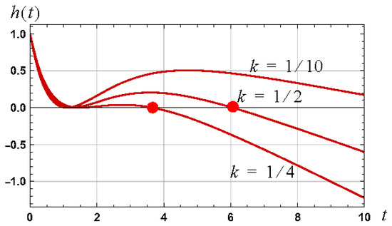
Figure 11. Graph of the impulse response of the transfer function defined by (69) for values of $k\in \left\{1/10,1/4,1/2\right\}$.

7. Summary of Results and Conclusion

7.1. Summary of Results

The approximations to $h_{r_0\left(y\right),r_1\left(y\right)}^{-1}\left(0\right)$, along with their associated relative error bounds, are detailed in Table 1. The associated approximations for the inverse Langevin function are detailed in Table 2.

Table 1. Summary of approximations for $h_{r_0\left(y\right),r_1\left(y\right)}^{-1}\left(0\right)$, as defined by (27) and (29) to (33), and their relative error bounds for the interval $\left[\mathrm{0,1}\right)$.

Approximation	Definition	Relative Error Bound	Relative Error Bound: 1st Order—(42)	Relative Error Bound: 2nd Order—(43)	Relative Error Bound: 3rd Order—(44)
$h_{{1,r}_0\left(y\right),r_1\left(y\right)}^{-1}\left(0\right)$	$\frac{-2}{1-y}·\left[1+y-y^2\right]$	$4.45\times {10}^{-2}$	$2.69\times {10}^{-4}$	$1.87\times {10}^{-5}$	$1.32\times {10}^{-6}$
$h_{{2,r}_0\left(y\right),r_1\left(y\right)}^{-1}\left(0\right)$	$\frac{-2}{1-y}·\left[1+c_{21}\sin \left(\pi y\right)+c_{22}\sin \left(\pi y^2\right)\right]$	$4.66\times {10}^{-3}$	$2.20\times {10}^{-4}$	$2.42\times {10}^{-5}$	$3.68\times {10}^{-6}$
$h_{{3,r}_0\left(y\right),r_1\left(y\right)}^{-1}\left(0\right)$	$\frac{-2}{1-y}·\left[1+y-y^2-\frac{y^{7/2}}{2}+\frac{y^{9/2}}{2}\right]$	$3.71\times {10}^{-3}$	$8.52\times {10}^{-6}$	$7.58\times {10}^{-8}$	$7.74\times {10}^{-10}$
$h_{{4,r}_0\left(y\right),r_1\left(y\right)}^{-1}\left(0\right)$	$\frac{-2}{1-y}·\left[1+y-y^2-\frac{y^4}{2}+y^6-\frac{y^7}{2}\right]$	$2.13\times {10}^{-3}$	$1.92\times {10}^{-6}$	$9.12\times {10}^{-9}$	$4.59\times {10}^{-11}$
$h_{{5,r}_0\left(y\right),r_1\left(y\right)}^{-1}\left(0\right)$	$\begin{array}{c}\frac{-2}{1-y}·\left[1+y-y^2-\frac{y^{7/2}}{2}+\frac{y^{9/2}}{2}\right]+\\ c_{51}{y}^5\left(1-y\right)(y-y_o)e^{-3{(y-y_o)}^2}\end{array}$	$2.33\times {10}^{-4}$	$3.15\times {10}^{-8}$	$1.68\times {10}^{-11}$	$1.04\times {10}^{-14}$
$h_{{6,r}_0\left(y\right),r_1\left(y\right)}^{-1}\left(0\right)$	$\begin{array}{c}\frac{-2}{1-y}·\left[1+y-y^2-\frac{y^4}{2}+y^6-\frac{y^7}{2}\right]·\\ \left[\begin{array}{l}1+{\alpha }_0{y}^2{(1-y)}^2\\ \left[\begin{array}{r}1+{\alpha }_2{y}^2+{\alpha }_3{y}^3+{\alpha }_4{y}^4+\\ {\alpha }_5{y}^5+{\alpha }_7{y}^7+{\alpha }_8{y}^8\end{array}\right]\end{array}\right]\end{array}$	$4.58\times {10}^{-5}$	4.07$\times {10}^{-10}$	$2.43\times {10}^{-14}$	$1.92\times {10}^{-18}$

Table 1. Summary of approximations for $h_{r_0\left(y\right),r_1\left(y\right)}^{-1}\left(0\right)$, as defined by (27) and (29) to (33), and their relative error bounds for the interval $\left[\mathrm{0,1}\right)$.

Approximation	Definition	Relative Error Bound	Relative Error Bound: 1st Order—(42)	Relative Error Bound: 2nd Order—(43)	Relative Error Bound: 3rd Order—(44)
$h_{{1,r}_0\left(y\right),r_1\left(y\right)}^{-1}\left(0\right)$	$\frac{-2}{1-y}·\left[1+y-y^2\right]$	$4.45\times {10}^{-2}$	$2.69\times {10}^{-4}$	$1.87\times {10}^{-5}$	$1.32\times {10}^{-6}$
$h_{{2,r}_0\left(y\right),r_1\left(y\right)}^{-1}\left(0\right)$	$\frac{-2}{1-y}·\left[1+c_{21}\sin \left(\pi y\right)+c_{22}\sin \left(\pi y^2\right)\right]$	$4.66\times {10}^{-3}$	$2.20\times {10}^{-4}$	$2.42\times {10}^{-5}$	$3.68\times {10}^{-6}$
$h_{{3,r}_0\left(y\right),r_1\left(y\right)}^{-1}\left(0\right)$	$\frac{-2}{1-y}·\left[1+y-y^2-\frac{y^{7/2}}{2}+\frac{y^{9/2}}{2}\right]$	$3.71\times {10}^{-3}$	$8.52\times {10}^{-6}$	$7.58\times {10}^{-8}$	$7.74\times {10}^{-10}$
$h_{{4,r}_0\left(y\right),r_1\left(y\right)}^{-1}\left(0\right)$	$\frac{-2}{1-y}·\left[1+y-y^2-\frac{y^4}{2}+y^6-\frac{y^7}{2}\right]$	$2.13\times {10}^{-3}$	$1.92\times {10}^{-6}$	$9.12\times {10}^{-9}$	$4.59\times {10}^{-11}$
$h_{{5,r}_0\left(y\right),r_1\left(y\right)}^{-1}\left(0\right)$	$\begin{array}{c}\frac{-2}{1-y}·\left[1+y-y^2-\frac{y^{7/2}}{2}+\frac{y^{9/2}}{2}\right]+\\ c_{51}{y}^5\left(1-y\right)(y-y_o)e^{-3{(y-y_o)}^2}\end{array}$	$2.33\times {10}^{-4}$	$3.15\times {10}^{-8}$	$1.68\times {10}^{-11}$	$1.04\times {10}^{-14}$
$h_{{6,r}_0\left(y\right),r_1\left(y\right)}^{-1}\left(0\right)$	$\begin{array}{c}\frac{-2}{1-y}·\left[1+y-y^2-\frac{y^4}{2}+y^6-\frac{y^7}{2}\right]·\\ \left[\begin{array}{l}1+{\alpha }_0{y}^2{(1-y)}^2\\ \left[\begin{array}{r}1+{\alpha }_2{y}^2+{\alpha }_3{y}^3+{\alpha }_4{y}^4+\\ {\alpha }_5{y}^5+{\alpha }_7{y}^7+{\alpha }_8{y}^8\end{array}\right]\end{array}\right]\end{array}$	$4.58\times {10}^{-5}$	4.07$\times {10}^{-10}$	$2.43\times {10}^{-14}$	$1.92\times {10}^{-18}$

Table 2. Summary of approximations, based on the approximations to $h_{r_0\left(y\right),r_1\left(y\right)}^{-1}\left(0\right)$ detailed in Table 1, for the inverse Langevin function along with their associated relative bounds for the interval $\left[\mathrm{0,1}\right)$. The relative error bounds for the first, second, and third order Schröder-based approximations arise from the direct use of the approximations in the general approximation form defined in Theorem 2.

Approx.	Definition	Relative Error Bound	Relative Error Bound: First Order	Relative Error Bound: Second Order	Relative Error Bound: Third Order
$L_1^{-1}\left(y\right)$	$\frac{3y}{1-y^2}·\left[1-\frac{y^2}{3}\right]$	$4.94\times {10}^{-2}$	$2.40\times {10}^{-3}$	$1.20\times {10}^{-4}$	$5.87\times {10}^{-6}$
$L_2^{-1}\left(y\right)$	$\frac{2y}{1-y^2}+\frac{d_{21}\sin \left(\pi y\right)+d_{22}\sin \left(\pi y^2\right)}{1-y}$	$1.83\times {10}^{-2}$	$2.94\times {10}^{-4}$	$5.29\times {10}^{-6}$	$9.23\times {10}^{-8}$
$L_3^{-1}\left(y\right)$	$\frac{3y}{1-y^2}·\left[1-\frac{y^2}{3}-\frac{y^{5/2}}{6}+\frac{y^{9/2}}{6}\right]$	$4.37\times {10}^{-3}$	$1.62\times {10}^{-5}$	$6.59\times {10}^{-8}$	$2.64\times {10}^{-10}$
$L_4^{-1}\left(y\right)$	$\frac{3y}{1-y^2}·\left[1-\frac{y^2}{3}-\frac{y^3}{6}-\frac{y^4}{6}+\frac{y^5}{3}+\frac{y^6}{6}-\frac{y^7}{6}\right]$	$2.44\times {10}^{-3}$	$5.32\times {10}^{-6}$	$1.24\times {10}^{-8}$	$2.84\times {10}^{-11}$
$L_5^{-1}\left(y\right)$	$\begin{array}{l}\frac{3y}{1-y^2}·\left[1-\frac{y^2}{3}-\frac{y^{5/2}}{6}+\frac{y^{9/2}}{6}\right]-\\ \frac{c_{51}{y}^5\left(1-y\right)(y-y_o)}{2}·e^{-3{(y-y_o)}^2}\end{array}$	$2.58\times {10}^{-4}$	$6.47\times {10}^{-8}$	$1.67\times {10}^{-11}$	$4.22\times {10}^{-15}$
$L_6^{-1}\left(y\right)$	$\begin{array}{l}\frac{3y}{1-y^2}·\\ \left[\begin{array}{c}1-\frac{y^2}{3}-\frac{y^3}{6}-\frac{y^4}{6}+\frac{y^5}{3}+\frac{y^6}{6}-\frac{y^7}{6}+\hfill \\ \frac{{\alpha }_{0}y{(1-y^2)}^2}{3}·\left[\begin{array}{c}\hfill 1-y^2+y^3-\frac{3y^4}{2}+\\ \hfill \frac{3y^5}{2}-\frac{y^6}{2}\end{array}\right]·\hfill \\ \hfill \left[\begin{array}{r}1+{\alpha }_2{y}^2+{\alpha }_3{y}^3+{\alpha }_4{y}^4+\\ {\alpha }_5{y}^5+{\alpha }_7{y}^7+{\alpha }_8{y}^8\end{array}\right]\end{array}\right]\end{array}$	$4.85\times {10}^{-5}$	$2.32\times {10}^{-9}$	$1.14\times {10}^{-13}$	$5.48\times {10}^{-18}$

Table 2. Summary of approximations, based on the approximations to $h_{r_0\left(y\right),r_1\left(y\right)}^{-1}\left(0\right)$ detailed in Table 1, for the inverse Langevin function along with their associated relative bounds for the interval $\left[\mathrm{0,1}\right)$. The relative error bounds for the first, second, and third order Schröder-based approximations arise from the direct use of the approximations in the general approximation form defined in Theorem 2.

Approx.	Definition	Relative Error Bound	Relative Error Bound: First Order	Relative Error Bound: Second Order	Relative Error Bound: Third Order
$L_1^{-1}\left(y\right)$	$\frac{3y}{1-y^2}·\left[1-\frac{y^2}{3}\right]$	$4.94\times {10}^{-2}$	$2.40\times {10}^{-3}$	$1.20\times {10}^{-4}$	$5.87\times {10}^{-6}$
$L_2^{-1}\left(y\right)$	$\frac{2y}{1-y^2}+\frac{d_{21}\sin \left(\pi y\right)+d_{22}\sin \left(\pi y^2\right)}{1-y}$	$1.83\times {10}^{-2}$	$2.94\times {10}^{-4}$	$5.29\times {10}^{-6}$	$9.23\times {10}^{-8}$
$L_3^{-1}\left(y\right)$	$\frac{3y}{1-y^2}·\left[1-\frac{y^2}{3}-\frac{y^{5/2}}{6}+\frac{y^{9/2}}{6}\right]$	$4.37\times {10}^{-3}$	$1.62\times {10}^{-5}$	$6.59\times {10}^{-8}$	$2.64\times {10}^{-10}$
$L_4^{-1}\left(y\right)$	$\frac{3y}{1-y^2}·\left[1-\frac{y^2}{3}-\frac{y^3}{6}-\frac{y^4}{6}+\frac{y^5}{3}+\frac{y^6}{6}-\frac{y^7}{6}\right]$	$2.44\times {10}^{-3}$	$5.32\times {10}^{-6}$	$1.24\times {10}^{-8}$	$2.84\times {10}^{-11}$
$L_5^{-1}\left(y\right)$	$\begin{array}{l}\frac{3y}{1-y^2}·\left[1-\frac{y^2}{3}-\frac{y^{5/2}}{6}+\frac{y^{9/2}}{6}\right]-\\ \frac{c_{51}{y}^5\left(1-y\right)(y-y_o)}{2}·e^{-3{(y-y_o)}^2}\end{array}$	$2.58\times {10}^{-4}$	$6.47\times {10}^{-8}$	$1.67\times {10}^{-11}$	$4.22\times {10}^{-15}$
$L_6^{-1}\left(y\right)$	$\begin{array}{l}\frac{3y}{1-y^2}·\\ \left[\begin{array}{c}1-\frac{y^2}{3}-\frac{y^3}{6}-\frac{y^4}{6}+\frac{y^5}{3}+\frac{y^6}{6}-\frac{y^7}{6}+\hfill \\ \frac{{\alpha }_{0}y{(1-y^2)}^2}{3}·\left[\begin{array}{c}\hfill 1-y^2+y^3-\frac{3y^4}{2}+\\ \hfill \frac{3y^5}{2}-\frac{y^6}{2}\end{array}\right]·\hfill \\ \hfill \left[\begin{array}{r}1+{\alpha }_2{y}^2+{\alpha }_3{y}^3+{\alpha }_4{y}^4+\\ {\alpha }_5{y}^5+{\alpha }_7{y}^7+{\alpha }_8{y}^8\end{array}\right]\end{array}\right]\end{array}$	$4.85\times {10}^{-5}$	$2.32\times {10}^{-9}$	$1.14\times {10}^{-13}$	$5.48\times {10}^{-18}$

7.2. Conclusions

The relationship between the inverse Langevin function and the r₀-r₁-Lambert W function was defined. The derived relationship leads to new approximations for the inverse Langevin function with potentially lower relative error bounds than comparable published approximations.

It was shown that improved approximations for the r₀-r₁-Lambert W function, with significantly lower relative error bounds, can be defined by utilizing Schröder’s root approximations of the first kind. Approximations for the inverse Langevin function can then be defined by utilizing the established relationship between the two functions. An alternative approach is to directly use an establish approximation for the inverse Langevin function in the general Schröder approximation form. Examples were given to illustrate that the former approach is likely to lead to a simpler analytical expression for a set relative error bound.

It was shown how the defined approximations for the inverse Langevin function can be utilized to establish approximations for the integral of the inverse Langevin function, with, in general, low relative error bounds.

The link between the inverse Langevin function and the r₀-r₁-Lambert W function was utilized to establish the roots of the impulse response of a custom linear system comprising an integrator, a cascade of two integrators, and a second order system.

In terms of future research, it is noted that iterative approaches can be utilized to establish approximations with lower relative error bounds and several results for the inverse Langevin function have been detailed, e.g., [14,21]. Berinda [26] and Gdawiec [27], for example, provide an overview of iterative approaches that can be utilized for fixed point problems. In general, iterative approaches lead to analytical approximations with a high degree of complexity and rely on an initial approximation. To achieve results with modest complexity, a low order of iteration is required along with an initial approximation that has a low relative error bound and with low complexity. New approximations, thus, are of interest and warrant ongoing research.

Appendix B.1. Case 1: 0 < y << 1

For the case of $0<y\ll 1$, and consistent with the left graph shown in Figure 4, the root of $h_{r_0\left(y\right),r_1\left(y\right)}$ that is of interest is close to, but left of, the known root of $-2/(1+y)$ (see (21)). Consider $h_{r_0\left(y\right),r_1\left(y\right)}\left(w\right)$, defined by (19), and the case of $h_{r_0\left(y\right),r_1\left(y\right)}\left(w\right)=0$, i.e.,

$$\frac{4e^{-2/\left(1+y\right)}}{{\left(1+y\right)}^2}+\frac{w(1-y)e^{-2/\left(1+y\right)}}{1+y}+w{e}^w=0.$$

(A10)

With the form for $w$ of $w=-2/(1+y)+\epsilon \left(y\right)$, it follows that:

$$\frac{4}{{\left(1+y\right)}^2}+\frac{1-y}{1+y}·\left[\frac{-2}{1+y}+\epsilon \left(y\right)\right]+\left[\frac{-2}{1+y}+\epsilon \left(y\right)\right]e^{\epsilon \left(y\right)}=0.$$

(A11)

Simplification, and a Taylor series expansion for the exponential function around the point zero, leads to:

$$2+\left(1-y\right)\epsilon \left(y\right)+\left[-2+\left(1+y\right)\epsilon \left(y\right)\right]\left[1+\epsilon \left(y\right)+\frac{{\epsilon }^2\left(y\right)}{2}+\cdots \right]=0.$$

(A12)

First, second, and third order expansions for the exponential function lead to the approximations:

$$\left\{\begin{array}{l}{\epsilon }^2\left(y\right)\left[1+y\right]=0, \mathrm{first} \mathrm{order}\\ {\epsilon }^2\left(y\right)\left[1+\frac{\left(1+y\right)\epsilon \left(y\right)}{2}\right]=0, \mathrm{second} \mathrm{order}\\ {\epsilon }^2\left(y\right)\left[y+\frac{\left(1+3y\right)\epsilon \left(y\right)}{6}+\frac{\left(1+y\right){\epsilon }^2\left(y\right)}{6}\right]=0, \mathrm{third} \mathrm{order}\end{array}\right.$$

(A13)

with solutions:

$$\left\{\begin{array}{l}\begin{array}{cc}\epsilon \left(y\right)=0,& \end{array}\mathrm{first} \mathrm{order}\\ \begin{array}{cc}\epsilon \left(y\right)=0,\epsilon \left(y\right)=\frac{-2y}{1+y},& \end{array}\mathrm{second} \mathrm{order}\\ \begin{array}{cc}\epsilon \left(y\right)=0,\epsilon \left(y\right)=\frac{-1-3y\pm \sqrt{1-18y-15y^2}}{2(1+y)},& \end{array}\mathrm{third} \mathrm{order}\end{array}\right.$$

(A14)

Consider the first non-zero solution for $\epsilon \left(y\right)$, which is the second order solution of $\epsilon \left(y\right)=-2y/(1+y)$. For the case of $y\to 0$, this solution implies $w=-2$, which is consistent with the root $-2/(1+y)$.

The third order solution, which is consistent with $\epsilon \left(y\right)\to 0,$ as $y\to 0$, is $\epsilon \left(y\right)=\frac{-1-3y+\sqrt{1-18y-15y^2}}{2(1+y)}\approx \frac{-6y-24y^2}{1+y}$ and leads to the approximation:

$$\begin{array}{cc}{h}_{r_0\left(y\right),r_1\left(y\right)}\left[\frac{-2-6y-24y^2}{1+y}\right]\approx 0,& 0<y\ll 1.\end{array}$$

(A15)

Hence:

$$h_{r_0\left(y\right),r_1\left(y\right)}^{-1}(0)\approx \frac{-2-6y-24y^2}{1+y}\approx -2-4y-20y^2$$

(A16)

after using the approximation ${\left(1+y\right)}^{-1}\approx 1-y+y^2.$

Appendix B.2. Case 2: y -> 1

For $y\approx 1$, Taylor series expansions around the point one yield the approximations:

$$\begin{array}{l}\begin{array}{c}{r}_0\left(y\right)=\frac{4e^{-2/(1+y)}}{{(1+y)}^2}\approx \end{array}\frac{1}{e}+\frac{1-y}{2e}+\frac{{\left(1-y\right)}^2}{8e}+\cdots \\ \begin{array}{c}{r}_1\left(y\right)=\end{array}\frac{(1-y)e^{-2/(1+y)}}{1+y}\approx \frac{1-y}{2e}-\frac{{\left(1-y\right)}^3}{16e}-\cdots \end{array}$$

(A17)

Substitution of these approximations into

$${h_{r_0\left(y\right),r_1\left(y\right)}\left(w\right)=r}_0\left(y\right)+r_1\left(y\right)w+w{e}^w=0$$

(A18)

yields

$$\frac{1}{e}+\frac{1-y}{2e}+\frac{{\left(1-y\right)}^2}{8e}+\cdots +\left[\frac{1-y}{2e}-\frac{{\left(1-y\right)}^3}{16e}-\cdots \right]w+w{e}^w=0.$$

(A19)

As $y\to 1$ from below, the require root of (A18) becomes increasingly negative (this is evident from a comparison of the left and right hand graphs shown in Figure 4). For the case of $\left|w\right|\gg 1$, and $w$ negative, the term $w{e}^w$ becomes vanishing small leading to

$$w\begin{array}{cc}=-\frac{\frac{1}{e}+\frac{1-y}{2e}+\frac{{\left(1-y\right)}^2}{8e}}{\frac{1-y}{2e}-\frac{{\left(1-y\right)}^3}{16e}}\approx \frac{-2}{1-y},& y=1-\mathsf{\Delta },0<\mathsf{\Delta }\ll 1,\end{array}$$

(A20)

and the required result

$$\begin{array}{cc}{h}_{r_0\left(y\right),r_1\left(y\right)}^{-1}\left(0\right)\approx \frac{-2}{1-y},& y=1-\mathsf{\Delta },0<\mathsf{\Delta }\ll 1.\end{array}$$

(A21)

Appendix C.1. Second Order

The second order Schröder approximation to $h$, as defined by Theorem 2, is

$$\begin{array}{l}{h}_2^{-1}\left(z\right)=h_1^{-1}\left(z\right)-{\left.\frac{{\left[h\left(w\right)-z\right]}^2{h}^{\left(2\right)}\left(w\right)}{2{\left[h^{\left(1\right)}\left(w\right)\right]}^3}\right|}_{w=h_0^{-1}\left(z\right)}\\ =\frac{{-r}_0\left(y\right)+w^2{e}^w+z}{r_1\left(y\right)+\left(1+w\right)e^w}-{\left.\frac{{\left[r_0\left(y\right)+r_1\left(y\right)w+w{e}^w-z\right]}^2(2+w)e^w}{2{\left[r_1\left(y\right)+\left(1+w\right)e^w\right]}^3}\right|}_{w=h_0^{-1}\left(z\right)}\end{array}$$

(A26)

and the approximation for the case of $z=0$ is

$$\begin{array}{c}{h}_2^{-1}\left(0\right)=\frac{{-r}_0\left(y\right)+w^2{e}^w}{r_1\left(y\right)+\left(1+w\right)e^w}-{\left.\frac{{\left[r_0\left(y\right)+r_1\left(y\right)w+w{e}^w\right]}^2(2+w)e^w}{2{\left[r_1\left(y\right)+\left(1+w\right)e^w\right]}^3}\right|}_{w=h_0^{-1}\left(0\right)}\end{array}$$

(A27)

Substitution for $r_0$ and $r_1$ yields:

$$\begin{array}{l}{h}_2^{-1}\left(0\right)=\frac{-4+{\left(1+y\right)}^2{w}^2\exp \left[w+\frac{2}{1+y}\right]}{1-y^2+{\left(1+y\right)}^2(1+w)\exp \left[w+\frac{2}{1+y}\right]}-\\ {\left. \frac{{\left[4+\left(1-y^2\right)w+{\left(1+y\right)}^{2}w\exp \left[w+\frac{2}{1+y}\right]\right]}^2(2+w)\exp \left[w+\frac{2}{1+y}\right]}{2(1+y){\left[1-y+(1+y)(1+w)\exp \left[w+\frac{2}{1+y}\right]\right]}^3}\right|}_{{w=h}_0^{-1}\left(0\right)}\end{array}$$

(A28)

Appendix C.2. Third Order

The third order Schröder approximation to $h$, as defined by Theorem 2, is

$$h_3^{-1}\left(\mathrm{z}\right)={\left.h_2^{-1}\left(z\right)-\frac{{\left[h\left(w\right)-z\right]}^3{h}^{\left(3\right)}\left(w\right) }{{6\left[h^{\left(1\right)}\left(w\right)\right]}^4}·\left[-1+\frac{3{\left[h^{\left(2\right)}\left(w\right)\right]}^2 }{h^{\left(1\right)}\left(w\right)h^{\left(3\right)}\left(w\right)}\right]\right|}_{{w=h}_0^{-1}\left(z\right)}$$

(A29)

and the approximation for the case of $z=0$ is

$$\begin{array}{l}{h}_3^{-1}\left(0\right)=h_2^{-1}\left(0\right)-\frac{{\left[r_0\left(y\right)+r_1\left(y\right)w+w{e}^w\right]}^2(3+w)e^w}{6{\left[r_1\left(y\right)+\left(1+w\right)e^w\right]}^4}·\\ \begin{array}{cc}& \begin{array}{cc}& {\left. \left[-1+\frac{3{(2+w)}^2{e}^{2w}}{\left[r_1\left(y\right)+\left(1+w\right)e^w\right](3+w)e^w}\right]\right|}_{w=h_0^{-1}\left(0\right)}\end{array}\end{array}\end{array}$$

(A30)

Substitution for $r_0$ and $r_1$ yields the required result:

$$\begin{array}{l}{h}_3^{-1}\left(0\right)=h_2^{-1}\left(0\right)-\\ {\left. \begin{array}{c}{\left[4+\left(1-y^2\right)w+{\left(1+y\right)}^{2}w\exp \left[w+\frac{2}{1+y}\right]\right]}^3\exp \left[w+\frac{2}{1+y}\right]·\\ \frac{\left[-(1-y)(3+w)+\left(1+y\right)(9+8w+2w^2)\exp \left[w+\frac{2}{1+y}\right]\right]}{6{(1+y)}^2{\left[1-y+(1+y)(1+w)\exp \left[w+\frac{2}{1+y}\right]\right]}^5}\end{array}\right|}_{{w=h}_0^{-1}\left(0\right)}\end{array}$$

(A31)

References

- Langevin, P. Sur la théorie du magnétisme. J. Phys. Theor. Appl. 1905, 4, 678–693. [Google Scholar] [CrossRef]
- Fiasconaro, A.; Falo, F. Analytical results of the extensible freely jointed chain model. Phys. A Stat. Mech.Appl. 2019, 532, 121929. [Google Scholar] [CrossRef]
- Iliafar, S.; Vezenov, D.; Jagota, A. Stretching of a Freely Jointed Chain in Two-Dimensions. arXiv 2013, arXiv:1305.5951. [Google Scholar]
- Itskov, M.; Dargazany, R.; Hornes, K. Taylor expansion of the inverse function with application to the Langevin function. Math. Mech. Solids 2012, 17, 693–701. [Google Scholar] [CrossRef]
- Nguessong, A.N.; Beda, T.; Peyraut, F. A new based error approach to approximate the inverse Langevin function. Rheol. Acta 2014, 53, 585–591. [Google Scholar] [CrossRef]
- Darabi, E.; Itskov, M. A simple and accurate approximation of the inverse Langevin function. Rheol. Acta 2015, 54, 455–459. [Google Scholar] [CrossRef]
- Jedynak, R. Approximation of the inverse Langevin function revisited. Rheol. Acta 2015, 54, 29–39. [Google Scholar] [CrossRef]
- Kröger, M. Simple, admissible, and accurate approximants of the inverse Langevin and Brillouin functions, relevant for strong polymer deformations and flows. J. Non-Newton. Fluid Mech. 2015, 223, 77–87. [Google Scholar] [CrossRef]
- Marchi, B.C.; Arruda, E.M. An error-minimizing approach to inverse Langevin approximations. Rheol. Acta 2015, 54, 887–902. [Google Scholar] [CrossRef]
- Rickaby, S.R.; Scott, N.H. A comparison of limited-stretch models of rubber elasticity. Int. J. Non-Linear Mech. 2015, 68, 71–86. [Google Scholar] [CrossRef]
- Petrosyan, R. Improved approximations for some polymer extension models. Rheol. Acta 2017, 56, 21–26. [Google Scholar] [CrossRef]
- Jedynak, R. A comprehensive study of the mathematical methods used to approximate the inverse Langevin function. Math. Mech. Solids 2018, 24, 1992–2016. [Google Scholar] [CrossRef]
- Marchi, B.C.; Arruda, E.M. Generalized error-minimizing, rational inverse Langevin approximations. Math. Mech. Solids 2019, 24, 1630–1647. [Google Scholar] [CrossRef]
- Howard, R.M. Analytical approximations for the inverse Langevin function via linearization, error approximation and iteration. Rheol. Acta 2020, 59, 521–544. [Google Scholar] [CrossRef]
- Mező, I.; Keady, G. Some physical applications of generalized Lambert functions. Eur. J. Phys. 2016, 37, 065802. [Google Scholar] [CrossRef]
- Mező, I. On the structure of the solution set of a generalized Euler–Lambert equation. J. Math. Anal. Appl. 2017, 455, 538–553. [Google Scholar] [CrossRef]
- Mező, I.; Baricz, Á. On the generalization of the Lambert W function. Trans. Am. Math. Soc. 2017, 369, 7917–7934. [Google Scholar] [CrossRef]
- Jamilla, C.; Mendoza, R.; Mező, I. Solutions of neutral delay differential equations using a generalized Lambert W function. Appl. Math. Comput. 2020, 382, 125334. [Google Scholar] [CrossRef]
- Petković, M.S.; Petković, L.D.; Herceg, Ð. On Schröder’s families of root-finding methods. J. Comput. Appl. Math. 2010, 233, 1755–1762. [Google Scholar] [CrossRef][Green Version]
- Dubeau, F. Polynomial and rational approximations and the link between Schröder’s processes of the first and second kind. Abstr. Appl. Anal. 2014, 2014, 719846. [Google Scholar] [CrossRef]
- Howard, R.M. Schröder based inverse function approximation. Axioms 2023, 12, 1042. [Google Scholar] [CrossRef]
- Corless, R.M.; Gonnet, G.H.; Hare, D.E.G.; Jeffrey, D.J.; Knuth, D.E. On the Lambert W function. Adv. Comput. Math. 1996, 5, 329–359. [Google Scholar] [CrossRef]
- Howard, R.M. Analytical Approximations for the Principal Branch of the Lambert W Function. Eur. J. Math. Anal. 2022, 2, 14. [Google Scholar] [CrossRef]
- Lóczi, L. Guaranteed-and high-precision evaluation of the Lambert W function. Appl. Math. Comput. 2022, 433, 127406. [Google Scholar]
- Schröder, E. Über unendlich viele Algorithmen zur Auflösung der Gleichungen. Math. Ann. 1870, 2, 317–365. [Google Scholar] [CrossRef]
- Berinde, V.; Takens, F. Iterative Approximation of Fixed Points; Springer: Berlin/Heidelberg, Germany, 2007. [Google Scholar]
- Gdawiec, K.; Kotarski, W.; Lisowska, A. Polynomiography based on the nonstandard Newton-like root finding methods. Abstr. Appl. Anal. 2015, 2015, 797594. [Google Scholar] [CrossRef]
Disclaimer/Publisher’s Note: The statements, opinions and data contained in all publications are solely those of the individual author(s) and contributor(s) and not of MDPI and/or the editor(s). MDPI and/or the editor(s) disclaim responsibility for any injury to people or property resulting from any ideas, methods, instructions or products referred to in the content. |
© 2024 by the author. Licensee MDPI, Basel, Switzerland. This article is an open access article distributed under the terms and conditions of the Creative Commons Attribution (CC BY) license (https://creativecommons.org/licenses/by/4.0/).