The objective of this study was accomplished by: (1) designing and administering a questionnaire for the forest manager of License 5 in order to obtain information regarding the forest management objectives for the forest, as well as his “best guess” of the forest value preferences of significant stakeholder groups; (2) designing and developing a weighting system suitable for goal programming using the analytic hierarchy process, a mathematical method for measuring preferences for diverse criteria in order to compare alternative decisions [
16], to transform stakeholders’ preferences into measurable weights; (3) determining targets of the goals using linear programming in a timber supply model (in Woodstock
TM); (4) formulating a GP model by modifying the existing timber supply model of License 5 and using the data from steps 2 and 3 as input to the model; and (5) evaluating the results of the GP model with four forest management scenarios: equal preference, individual stakeholder preference, group average preference, and weighted average preference scenarios.
3.2. Step Two: Weight Determination Using Analytic Hierarchy Process
The objective of this step was to translate the forest manager’s best guess of the relative preference of each stakeholder group for the four FM goals into measurable weights by applying the AHP, employing an adaptation of the methodology described by Smith and Lantz [
18]. The AHP made it possible to assign weights to this ranking of predefined forest values [
16]. A “goal-weighting matrix” was formed by making pair-wise comparisons using a five-point scale (having numerical preference scores of 1, 3, 5, 7, and 9 for stated preferences of equal, weak, strong, and very strong respectively) to determine the weight of each goal. In this study, the value of a preference score to a given goal varied from 1 to 9, where 1/1 indicates equal importance, 3/1 weakly greater importance, 5/1 strongly greater importance, 7/1 very strongly greater importance, and 9/1 absolutely greater importance. The following describes the procedure using the predicted preferences of the Environmentalist group of stakeholders.
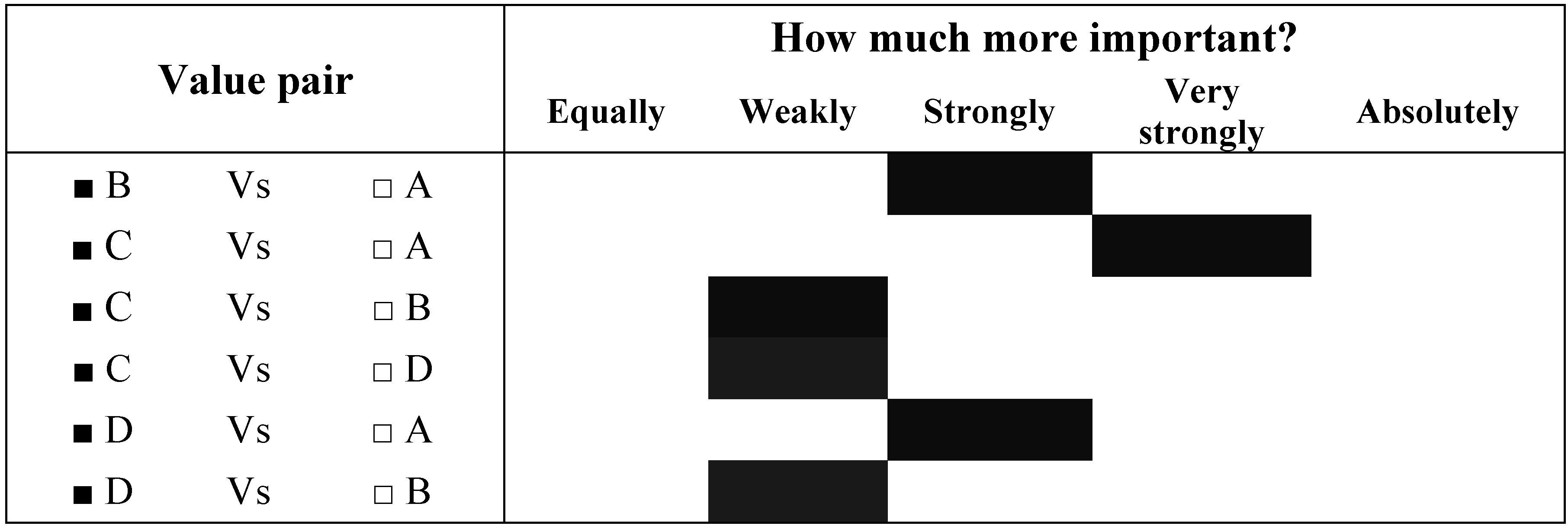
Task 1: Enter the subjective preferences of the Environmentalist group (as simulated by the forest manager) for the four FM goals (e.g., timber, employment, old spruce-fir habitat (OSFH), and scenic beauty representing letters A, B, C, and D in
Figure 1). According to this group’s (simulated) preferences, B is preferred to A, C is preferred to A, B and D, and D is preferred to both A and B. More specifically, according to the level of importance, B (checked) is strongly more important than A, C (checked) is very strongly more important than A, C is weakly more important than both B and D, and D (checked) is strongly and weakly more important than A and B respectively.
Figure 1.
Simulated preferences of the Environmentalist group.
Figure 1.
Simulated preferences of the Environmentalist group.
Task 2: Convert the preferences to numerical values and sum the column elements (see
Table 1). Here, B is 5 times more important than A (since B is strongly more important than A); C is 7 times more important than A (since C is very strongly more important than A); and D is 5 times more important than A (since D is strongly more important than A); By summing the column elements for A (second column in the table), the total value in Column A became 18.00 (1 + 5 + 7 + 5). In a similar way, the total values for columns B, C and D were measured.
Table 1.
Weightings derived from the simulated preferences of the Environmentalist group.
Table 1.
Weightings derived from the simulated preferences of the Environmentalist group.
| Values | A | B | C | D |
|---|
| A | 1 | 1/5 | 1/7 | 1/5 |
| B | 5 | 1 | 1/3 | 1/3 |
| C | 7 | 3 | 1 | 3 |
| D | 5 | 3 | 1/3 | 1 |
| Total | 18.00 | 7.200 | 1.808 | 4.533 |
Task 3: Divide each element by its column total. Averaging each row provides the normalized priority weight for the corresponding value. The highest number under the priority column indicates the highest preference.
For example, by dividing each element in row A (1, 5, 7, and 5) by the corresponding column total of A (18.00), three values were found viz. 0.0556, 0.2778, 0.3889, and 0.2778 (see
Table 2). In this case, the normalized priority weight for A is 0.051 ((0.0556 + 0.2778 + 0.3889 + 0.2778)/4).
Table 2.
Normalized weightings derived from the preferences of the Environmentalist group.
Table 2.
Normalized weightings derived from the preferences of the Environmentalist group.
| Values | A | B | C | D | Normalized priority/weight (∑ = 1) |
|---|
| A | 0.055556 | 0.027777 | 0.0785398 | 0.0441208 | 0.051 |
| B | 0.277778 | 0.138888 | 0.1841814 | 0.0734612 | 0.169 |
| C | 0.388889 | 0.416666 | 0.5530973 | 0.6618133 | 0.505 |
| D | 0.277778 | 0.416666 | 0.1841814 | 0.2206044 | 0.275 |
The steps mentioned above were applied to this research to determine the priority weight of each goal by each stakeholder group (see
Table 3). However, the preferences of the stakeholder groups were not checked for internal consistency, a problem that can occur regardless of the source of the preferences when the AHP method is used (for a discussion of the problems of AHP and how these might be identified and rectified using eigenvalues and consistency coefficients, see Saaty, [
16]). A thorough analysis of the internal consistency of the forest manager’s estimates of the stakeholders’ preferences was beyond the scope of this research project. However, if the proposed methodology is to be used in an actual exercise that involves ‘live’ stakeholders and that depends upon more certain knowledge of their actual values, then checking for internal consistency of the preferences would be advisable. Note that an IDM approach (mentioned in the introduction) may also be applicable since it would allow us to choose goal targets directly from stakeholders (through comparisons of the tradeoffs between competing objectives) rather than asking them for their preferences for each goal. However, the IDM approach is more suitable for a situation where it would be possible to have the “live”, ongoing involvement of all stakeholders.
Table 3.
Preferential weights of all stakeholder groups determined by the AHP.
Table 3.
Preferential weights of all stakeholder groups determined by the AHP.
| Goal | Stakeholders’ preferential weights (normalized to 1.00) |
|---|
| Licensee | NB Govt. | Local communities | Recreationists | Environmentalist |
|---|
| Timber | 0.642 | 0.290 | 0.106 | 0.047 | 0.051 |
| Employment | 0.218 | 0.540 | 0.449 | 0.093 | 0.169 |
| OSFH | 0.093 | 0.105 | 0.121 | 0.199 | 0.505 |
| Scenic beauty | 0.047 | 0.065 | 0.324 | 0.661 | 0.275 |
3.3. Step Three: Linear Programming Modeling
The objective of this section is to perform modeling by linear programming (LP) in order to determine the maximum possible values that could be achieved for each of the four goals over an 80-year planning horizon based on an existing timber supply model of Crown License 5. The original timber supply model (actually implemented in 2002) was modified to formulate LP and GP models for this research (see Hossain [
17] for details of the original and modified models).
Some constraints used by the Licensee were removed from the original timber supply model for two reasons: (I) they had been added to the original model for operational rather than policy reasons (for example, to meet the silvicultural budget constraints stipulated by the government), and (II) they might tend to over-constrain the model and thereby cloud the results of this research. For these reasons, all silvicultural constraints were removed from the original timber supply model in order to develop the LP and GP models for this study. The area of OSFH constraint was also removed since it was one of the goals of the multi-objective models. Thus, the constraints removed from the original model were: plantation area, commercially thinned area, spacing area, pre-commercially thinned area, and area of OSFH. Other constraints (e.g., medium wintering deer habitat, severe-wintering deer habitat, mature pine area, mature cedar area, mature jack pine area, mature spruce area, and buffer volume constraint) were retained to satisfy government requirements. A non-declining yield constraint was added to the model to prevent any reduction of timber supply over the planning horizon and a constraint ensuring that the growing stock in the final inventory was greater than or equal to the average of the last fifteen periods was imposed.
The FM goals were measured in terms of specific indicators. The indicator for the timber goal was total timber (m
3) harvested (both softwood and hardwood) over the planning horizon (16 five-year planning periods). The employment goal was calculated from the total number of work hours required for all FM activities (e.g., timber harvesting, planting, commercial thinning, transportation, and primary wood processing activities in the mill). The OSFH goal was the sum, for all periods, of the area (ha) of forests 65–185 years of age conforming to the definition of old spruce-fir habitat according to the original timber supply model. Incorporation of forest scenic beauty into an MOFM process requires that scenic beauty be defined in terms of stand characteristics [
19]. While several studies have been undertaken to predict scenic beauty as a social value, the indicators used to define it are somewhat arbitrary. Sheppard
et al. [
20] have used cut area size and regeneration age and height as quantitative indicators for scenic beauty and/or aesthetic value of forests according to Sustainable Forest Initiative (SFI)
TM standards. Brown and Daniel [
19] have found that mature and even-aged stands were aesthetically pleasing to visitors to the forest. Buhyoff
et al. [
21] have reported that, in southern pine stands in North Carolina, although stand scenic beauty was correlated with stand age, stem size and basal area, only stand-age seemed to have a significant relationship with stand scenic beauty. Since stand age was found to be the dominant factor affecting scenic value of forests in the studies described earlier and no documented research was found that defined scenic beauty in terms of stand characteristics in Canada, stand age was used as a surrogate measure of scenic beauty in this research, with stands between the ages of 20 to 100 years considered to be “scenically beautiful”.
Four LP models for the License were developed using Woodstock
TM (Remsoft 3.27 version) and the MOSEK LP solver. In addition to the model using the same objective function as was defined in the original timber supply model (maximize total harvest of timber over the 80 year planning horizon), three other models for the same planning period were created that used other objective functions: (1) maximize total employment, (2) maximize total scenic beauty area, and (3) maximize total area of OSFH. First, the timber goal was maximized without regard to other goals subject to the constraints described previously. In the subsequent models, each other goal (e.g., OSFH, employment, and scenic beauty) was maximized without regard to other goals, all subject to the same constraints. The outcomes of all LP models, shown in terms of total values of each goal when they are maximized in isolation over the 80 year planning horizon, are presented in
Table 4. These values were used as goal targets in the goal programming model.
3.4. Step Four: Goal Programming Modeling
The intent of this step was to perform goal programming to identify multiobjective solutions based upon different weighting schemes. The GP model was formulated using the outcomes obtained from LP models
(see
Section 3.3) as the goal targets. Before adding preference weightings, all goals were normalized to ensure that the value of deviations from targets for each goal would be equal when the goals themselves were equally preferred. This was done by adopting a modified version of the process developed by Balteiro and Romero [
22]. A detailed description of the goal normalization process can be found in Hossain [
17]. The normalized weight of each goal obtained from this process is presented in the second numeric column in
Table 4.
Table 4.
Maximum total output and normalized weights of each goal in LP modeling over the 80 year planning horizon.
Table 4.
Maximum total output and normalized weights of each goal in LP modeling over the 80 year planning horizon.
| Goals | Maximum total output of each goal | Normalized weights |
|---|
| Timber (m3) | 10,223,481 | 1 |
| Employment (work-hours) | 2,641,528 | 14.28 |
| OSFH (ha) | 415,168 | 16.39 |
| Scenic beauty (ha) | 807,005 | 26.31 |
The goals were then weighted under four weighting schemes: equal preference, individual stakeholder preference (ISP), group average preference (GAP), and weighted average preference (WAP). In the equal preference scenario, all the objectives were given equal preference, regardless of the preferences of the various stakeholders, so each of the four goals had a weight of 0.25. The GAP and WAP scenarios were developed to imply consensus among the stakeholder groups. In the GAP scenario, the preferential weight of each goal was determined by averaging the weights (determined by the AHP) across the stakeholder groups. This scenario was developed to examine how the achievement of a goal could be impacted when a combined value of the preferences of all stakeholder groups is considered regardless of their size. In the WAP scenario, the preferential weight of each goal was modified based on the number of people represented by each group. The rationale for developing the WAP scenario was to investigate how the FM decision-making processes could be influenced when stakeholders’ preferences are affected by the size of the stakeholder groups. In the ISP set of scenarios, the preferential weight of each stakeholder group, as determined by the AHP, was applied to determine the preferred solution of each individual stakeholder group.
In order to elicit the final weights (or penalty points for not achieving goals in GP) to be attached to each goal, we implemented a multiplicative aggregation process [
22] between the preferential weights (obtained from AHP) and normalized weights (obtained from goal normalization). In all FM scenarios (e.g., equal preference, ISP, GAP, and WAP), the final weight for each goal was determined by multiplying the preferential weight with the normalized weights. The weightings used are presented in
Table 5.
Table 5.
Final weight of each goal under GAP, WAP and ISP scenarios.
Table 5.
Final weight of each goal under GAP, WAP and ISP scenarios.
| Goal | Final weight of each goal |
|---|
| GAP | WAP | Licensee | NB Govt. | Local communities | Recr. groups | Envi. groups |
|---|
| Timber | 0.227 | 0.196 | 0.642 | 0.290 | 0.106 | 0.047 | 0.051 |
| Employment | 4.241 | 5.526 | 3.113 | 7.711 | 6.411 | 1.328 | 2.413 |
| OSFH | 3.343 | 2.245 | 1.524 | 1.720 | 1.983 | 3.261 | 8.276 |
| Scenic beauty | 7.208 | 9.945 | 1.236 | 1.710 | 8.524 | 17.390 | 7.235 |
Goal programming modeling was performed to minimize the weighted sum of deviations of each goal from its target based upon different weighting schemes. Goal deviations indicate the difference between the maximum value of a goal and what could be accomplished with respect to the goal (a description of the goal constraints and the deviation variables can be found in Hossain [
14]). The reason to employ GP is that it allowed us to express multiple and conflicting goals in a model to find feasible solutions. Unlike LP, where feasible solutions can only be achieved if the goal constraints are satisfied, GP doesn’t require that the goal targets be strictly achieved. The general design of the objective function in the GP is given as:
where,
![Forests 01 00099 i002]() = positive deviation of ith goal from its target (i = 1…4) = positive deviation of ith goal from its target (i = 1…4) |
![Forests 01 00099 i003]() = negative deviation of ith goal from its target (i = 1…4) = negative deviation of ith goal from its target (i = 1…4) |
| Wi = weights of ith goal (i = 1…4) |
The goal achievement levels for 16 periods (80 years) under the equal preference, GAP and WAP scenarios are presented in
Table 6, while those of the ISP scenarios are presented in
Table 7. It is noteworthy that in the GP models in this study, the goal targets and goal achievements were the aggregate measures of each goal over all periods. In an actual situation, it is very likely that constraints would also be set on the minimum achievement of each goal in each period, as well as on the maximum variation in goal achievement between periods. In this “proof of concept” study, however, the only periodic goal that was constrained to be above a minimum was that of OSFH, as had been noted earlier.
Table 6.
Total achievement value of each goal in the equal preference, GAP, and WAP scenariosa.
Table 6.
Total achievement value of each goal in the equal preference, GAP, and WAP scenariosa.
| Weightingschemes | Total goal achievement levels in the GP models |
|---|
| Timber (m3) (10,223,475)a | Employment (work-hours) (2,641,520) | OSFH (ha) (415,165) | Scenic beauty (ha) (807,000) |
|---|
| Equal preference | 10,133,518 | 2,487,181 | 72,951 | 647,821 |
| (99.12%)b | (94.15%) | (17.57%) | (80.27%) |
| GAP | 9,118,488 | 2,613,684 | 131,656 | 709,888 |
| (89.19%) | (98.94%) | (31.71%) | (87.96%) |
| WAP | 9,119,018 | 2,615,615 | 127,087 | 710,294 |
| (89.20%) | (99.01%) | (30.61%) | (88.01%) |
Table 7.
Total achievement value of each goal in the ISP scenarios.
Table 7.
Total achievement value of each goal in the ISP scenarios.
| Stakeholder groups | Total goal achievement levels in the GP models |
|---|
| Timber (m3) (10,223,475)a | Employment (work-hours) (2,641,520) | OSFH (ha) (415,165) | Scenic beauty (ha) (807,000) |
|---|
| Licensee | 9,793,863 | 2,597,025 | 84,306 | 669,826 |
| (95.79%)b | (98.31%)b | (20.30%)b | (83.00%)b |
| NB Government | 9,291,713 | 2,640,833 | 90,544 | 689,120 |
| (90.88%) | (99.97%) | (21.80%) | (85.39%) |
| Local communities | 9,152,874 | 2,622,293 | 115,597 | 707,851 |
| (89.52%) | (99.27%) | (27.84%) | (87.71%) |
| Recreationalgroups | 7,475,307 | 2,226,253 | 213,477 | 766,294 |
| (73.11%) | (84.27%) | (51.41%) | (94.95%) |
| Environmentalgroups | 7,999,893 | 2,366,572 | 219,354 | 742,869 |
| (78.25%) | (89.59%) | (52.83%) | (92.05%) |
3.5. Step Five: Evaluation of Goal Programming Results
In this step, the multi-objective solutions obtained from goal programming modeling were assessed. Upon analysis of
Table 6 and
Table 7, it was found that the achievement of only one goal, OSFH, varied significantly in terms of percentage of the goal target across the equal preference, GAP, WAP, and ISP model runs. As expected, it was observed that in none of the MOFM scenarios were the individual goal targets completely achieved since the MOFM process requires making trade-offs among individual goals in order to attain a global optimum solution.
The results in
Table 6 show how the achievement (total value) of all goals vary under different weighting methods (equal preference, GAP and WAP scenarios). As could be expected, the achievement of employment and scenic beauty is improved in the GAP and WAP scenarios compared to the equal preference scenario simply because the weights of those goals are higher in these scenarios. However, the relationship of weights to final results are not similarily consistent for the timber and OSFH goals. Possible reasons for this will be discussed later.
In
Table 7, which shows the results of the ISP runs where each stakeholder’s preferences were used to weight individual multi-objective model runs, it is observed that the relative achievement of each goal in the ISP scenarios is consistent with the relative preferences of the stakeholder groups (as seen in
Table 5). Here, the total values of timber, employment, scenic beauty, and OSFH are maximum for the Licensee, NB Government, recreational groups, and environmental groups respectively, since these are the most preferred goals of the stakeholder groups. Conversely, the achievement of OSFH and scenic beauty is lowest for the Licensee, since these are the least preferred goals for that stakeholder. Similarly, the achievement of employment is lowest for the recreational groups, since this is the least preferred goal for recreational groups (
Table 3 and
Table 5).
In terms of deviation of goal outputs (total value) from the targets, the deviation of OSFH output is greatest compared to other goals (82 % deviation from the target; see
Table 6 and
Table 7). One reason of this low achievement could be that the age-range of the occurrance of OSFH is 65–185 years while most harvesting actions are carried out on stands aged 70–170 years, so logically it is difficult to achieve OSFH and timber simultaneously. Given that employment and timber are closely related since most employment comes from timber production, their combined weight would tend to surpass that of OSFH. For instance, in the GAP and WAP scenarios, the combined weights of employment and timber are 4.468 and 5.722 respectively, which are much higher than the weights of OSFH (
Table 5). Clearly, this combined weight should exert a negative influence on the attainment of OSFH. However, this does not completely explain why the maximum achievement of OSFH is only 18% of its target in the equal preference scenario.
Upon performing a series of equal preference GP models with minimum OSFH level (total OSFH must be greater than or equal to 125,000; 150,000; 175,000; 200,000; 225,000 and, 250,000 ha), it was observed that the achievement of timber decreased sharply to zero when the OSFH constraint was set to 250,000 ha, implying that after this point the cost of losing timber rises suddenly and dramatically (
Table 8). This would be a major reason why the achievement of OSFH is so poor when all four goals are targeted simultaneously; that is to say that after a certain point (i. e. when OSFH is greater than or equal to 250,000 ha) the cost of losing timber (and/or employment since timber and employment are closely related) is so high that the model favours achieving timber at the expense of OSFH. However, given the multi-dimensional nature of the model and the complexity of the forest, it is not possible explain exactly how the trade-offs were made among the goals.
Table 8.
Total values of OSFH and timber at minimum OSFH constraints.
Table 8.
Total values of OSFH and timber at minimum OSFH constraints.
| Total value of OSFH(ha) | Total value of timber (m3) | Minimum OSFH constraint(ha) |
|---|
| 246,320 | 7,091,712 | OSFH ≥ 125,000 |
| 247,792 | 7,084,528 | OSFH ≥ 150,000 |
| 249,456 | 7,078,416 | OSFH ≥ 175,000 |
| 252,512 | 7,063,184 | OSFH ≥ 200,000 |
| 259,744 | 6,979,712 | OSFH ≥ 225,000 |
| 315,008 | 0 | OSFH ≥ 250,000 |


 = positive deviation of ith goal from its target (i = 1…4)
 = negative deviation of ith goal from its target (i = 1…4)