Article

Comparison of RegCM4.7.1 Simulation with the Station Observation Data of Georgia, 1985–2008

by
Mariam Elizbarashvili
1,*,
Avtandil Amiranashvili
2,
Elizbar Elizbarashvili
3,
George Mikuchadze
1,
Tamar Khuntselia
1 and
Nino Chikhradze
1
1
Faculty of Exact and Natural Sciences, Ivane Javakhishvili Tbilisi State University, 0179 Tbilisi, Georgia
2
M. Nodia Institute of Geophysics, Ivane Javakhishvili Tbilisi State University, 0160 Tbilisi, Georgia
3
Climatology and Agroclimatology Department, Institute of Hydrometeorology, Georgian Technical University, 0112 Tbilisi, Georgia
*
Author to whom correspondence should be addressed.
Atmosphere 2024, 15(3), 369; https://doi.org/10.3390/atmos15030369
Submission received: 31 January 2024 / Revised: 28 February 2024 / Accepted: 7 March 2024 / Published: 18 March 2024

Abstract

:
The global climate change, driven by natural processes and increasing human activities, is especially significant for Georgia. The region is experiencing increases in temperature, desertification, redistribution of precipitation, and a rise in the frequency and severity of extreme weather events. Georgia’s complex topography and its proximity to the Black and Caspian seas make it essential to employ high-resolution regional climate models to evaluate future climate change risks. In this study, we examine the results of a high-resolution simulation of mean and extreme precipitation and temperature using the Abdus Salam International Centre for Theoretical Physics Regional Climate Model version 4.7.1 for the period 1985–2008, providing an initial evaluation of the model’s performance for the territory of Georgia. The model domain (1524 km; 2388 km) encompasses the entirety of Georgia’s territory and surrounding regions. The simulation, conducted at a 12 km horizontal grid spacing using ERA5 data as boundary conditions, indicates that the least discrepancy between observed and modeled average annual temperatures and precipitation, falling within a −1 to 1 °C and −200 to 200 mm range, respectively, was observed at most stations of eastern Georgia. The largest disparities between the model and observed average annual precipitation totals were noted along the Black Sea coast, in the Kolkheti Lowland, and in some high mountain stations in western Georgia. The most significant differences in average annual temperatures between the model and observations were observed in Ambrolauri, Mt. Sabueti, and Dedoplistskaro. For Georgia territory, such a long run with such a high resolution using ERA5 as boundary conditions was conducted for the first time. Overall, the modeling results are quite satisfactory, providing a solid basis for the successful utilization of the regional climate model RegCM4.7.1 with the selected parameterization for modeling monthly mean and extreme temperatures and precipitation in Georgia.

1. Introduction

Georgia is a country in the South Caucasus region. The Black Sea borders it to the west, the Greater Caucasus Range to the north, and the Lesser Caucasus to the south. The Greater Caucasus is connected with the Lesser Caucasus by the Likhi range, which divides the country into two physical–geographical areas: western Georgia and eastern Georgia. Humid subtropical climatic conditions characterize the western part of Georgia, while eastern Georgia is characterized by transitional from humid to dry subtropical climatic conditions [1]. The direction of the main ranges of the Caucasus greatly influences the climate and atmospheric circulation in the lower layers of the troposphere in the territory of Georgia, which practically specifies the trajectories of the movements of air masses. In particular, the penetration of air masses from western [2] and eastern directions prevails here. Bilateral penetration of air masses in the territory of Georgia is very rare [1]. The Greater Caucasus typically acts as a formidable obstacle for the air masses coming from the north, while the air masses coming from the south are attenuated by the Lesser Caucasus, allowing them to disperse more freely, particularly in the higher atmospheric layers [3].
Georgia exhibits a high sensitivity to climate change, with noticeable changes already observed, largely attributable to its complex topography and proximity to the sea [1]. Georgia is experiencing increases in temperature, desertification, redistribution of precipitation, a rise in the frequency and severity of extreme weather events, etc. [4,5,6]. Specifically, temperatures are increasing faster in the arid landscapes of eastern Georgia than in the humid landscapes of western Georgia [1]. Since the 1960s, monthly minimum temperatures have risen by 0.22 °C and maximum temperatures by 0.36 °C. Warm extremes have exhibited greater fluctuations and trends compared to cold extremes [5,6]. At the same time, over the past 50 years, Georgia has experienced a significant increase in the intensity, frequency, and duration of heat waves. The frequency of heat waves has risen by 0.7 events per decade, while the duration has increased by 4.3 days per decade per event [4,5,6]. Precipitation in western Georgia essentially has increased, whereas in eastern Georgia, it has decreased [1]. Furthermore, in eastern Georgia, the severity of drought has increased markedly in the past 30 years; the annual duration of the dry season has increased from 54 to 72 days, and the frequency of its occurrence has risen two-fold [7]. As a result of these changes, many areas in eastern Georgia currently face water shortages [7,8]. Given Georgia’s complex topography, coastlines, hydrology, and circulation processes, high-resolution regional climate modeling is necessary for climate change assessments.
Within the Second National Communication to the UNFCCC of Georgia, the regional climate model—PRECIS (Providing Regional Climates for Impacts Studies) was used over the South Caucasus domain at a 25 km horizontal resolution for the 1961–1990 historical period with boundary conditions: ERA40 and the obtained results were validated by comparing model data to the Climatic Research Unit (CRU) data [7,9,10]. The study results show that in the case of temperature, CRU data exceeded the simulated data obtained from PRECIS for both western and eastern Georgia. In some places, the difference in average annual temperatures exceeded 7 °C. For precipitation, a significant difference between the model and CRU data was observed on the Black Sea coast, where the precipitation calculated by the PRECIS model was two times less [7].
The two future runs (2020–2050 and 2070–2100) were conducted for IPCC SRES A1, A2, and B1, B2 [11] climate scenarios. Based on these simulations, the average values of major climatic parameters were analyzed over Georgia territory [7].
Within the Third National Communication to the UNFCCC of Georgia, the Abdus Salam International Centre for Theoretical Physics (ICTP) regional climate model RegCM4 was used at 20 km horizontal resolution for a South Caucasus domain for the future periods 2021–2050 and 2071–2100; however, historical runs and model validation have not been performed. Mean values of main climate parameters and extreme climate indices have been analyzed in this study for the historical period 1986–2010 based on 33 meteorological stations of [8], and future changes have been analyzed comparing model data (2021–2050 and 2071–2100) to meteorological observation data (1986–2010) [8]. First of all, this approach is not acceptable for climate change assessment, and the 20 km horizontal resolution is quite coarse for climate change assessments for Georgia. Climate models of higher resolution provide a more accurate depiction of land surface diversity and detailed influences, crucial for precise simulation of local and regional climate characteristics [9,12].
Performing historical simulations and validating the model are essential stages in guaranteeing the dependability and precision of climate model forecasts [13]. Failing to conduct historical simulations and validate model outputs against observed data leads to heightened uncertainty regarding the model’s capability to accurately replicate past climate conditions [14]. This absence of validation undermines the reliability of future projections and constrains trust in the model outcomes.
In this study, we conducted RegCM4.7.1 simulation at 12 km resolution for Georgia, covering the historical period, and evaluated a 24-year (1985–2008) simulation of annual and monthly mean and extreme temperatures and precipitation from the model against meteorological station observation data in Georgia.
The modeling results, in general, can be considered quite satisfactory, which gives grounds for successfully using the regional climate model RegCM4.7.1 with selected parameterization when modeling monthly mean and extreme temperatures and precipitation in Georgia.
This marks a significant initial step toward generating high-resolution future climate projections for Georgia.
This study holds great importance from both scientific and societal viewpoints, as it lays the groundwork for (1) providing in the future the highest resolution climate information for the Georgian region, (2) providing quality impact-level information and assessments important for local stakeholders and regional and global policymakers, and (3) advancing the field of climate change, not only in Georgia but also on an international scale.

2. Materials and Methods

2.1. The Regional Climate Model

RegCM is a regional climate model initially created by the National Center for Atmospheric Research (NCAR) and currently maintained by the Abdus Salam International Centre for Theoretical Physics (ICTP) [15,16,17,18,19]. It has been extensively employed in regional climate research across various regions worldwide and has been selected as one of the RCMs for the Coordinated Regional Climate Downscaling Experiment (CORDEX) [20,21,22,23,24,25,26,27,28].
In this study, we applied the Regional Climate Model version 4.7.1. The parameterization schemes for the simulation consist of the Holtslag boundary layer scheme [29,30], Zeng ocean fluxes scheme [31], Tiedtke cumulus convection scheme over land [32], WSM5 moisture scheme [33,34], RRTM radiation scheme [35,36] and the Community Land Model scheme CLM4.5 [37].
The RegCM4.7.1. simulation was carried out from 1 January 1984 to 31 December 2008 at a horizontal grid spacing of 12 km using a non-hydrostatic dynamic core [38,39]. The first year, 1984, was used as a spin-up period to ensure that all components of the regional climate model reached physical equilibrium under the applied forcing. The results for the period 1985–2008 were then analyzed. ERA5 high-resolution atmospheric reanalysis data from the European Centre for Medium-Range Weather Forecasts (ECMWF) and sea surface temperature data of the National Oceanic and Atmospheric Administration (NOAA) [40] were employed as initial and lateral boundary conditions. The domain consists of 41 vertical levels, with the model top set at 15 hPa. The center of the simulated area is located at Clat = 41.5 N, Clong = 41.2 E, and the number of grid cells is 200 in the east–west direction and 128 in the north–south direction.
The model domain encompasses the entirety of Georgia’s territory and surrounding regions, including key topographical features such as the Caucasus Mountains, as well as the entire Black and Caspian seas (25.67–56.89 N, 34.10–48.24 E). Figure 1 illustrates the RegCM domain, topography, and Georgia’s location in the region. These parameterizations were chosen in previous studies [41,42,43,44,45]. We carried out several short-term simulations of RegCM for the territory of Georgia with different parameterizations, and we also compared the outcomes of these simulations with the observational data of weather stations in Georgia [41,42,43,44,45]. As a result, we selected the most optimal parameterization and domain size both from the point of view of computer resources and the best outcome.

2.2. Weather Station Data

The research used the observation data of 21 meteorological stations on the territory of Georgia for the years 1985–2008, in particular, the annual and monthly mean and extreme temperatures and precipitation.
Observations at the meteorological stations of Georgia are carried out under the guidance of the National Environmental Agency (https://nea.gov.ge/En) (accessed on 6 March 2024). The National Environmental Agency checks the observational data for quality with an environment-based R script (software). The agency uses data from 21 stations located in the territory of Georgia for climate analysis and sends the information to the WMO. At these stations, long-term observations are conducted using standard meteorological instruments. Temperature data are collected every 3 h, and precipitation data are collected twice a day. In the last few years, automatic meteorological stations have also been installed on some of them. The data of the National Environmental Agency are available to scientific institutions without any fees. We used the data of instrumental observations of 20 of these 21 stations in our research, as there are complete temperature and precipitation data for 20 stations for the years 1985–2008: a continuous homogeneous series.
Table 1 presents the coordinates and altitude above sea level of the meteorological stations used in this study. It also indicates the climatic zone in which each station is situated [46].
In this study, the observational data from 20 weather stations were compared with the data from the nearest grid point in the model simulation. Correlation analysis and comparative analysis methods were used to compare the model and observation data. In addition, mathematical statistics methods were used in the work, which allowed us to study the statistical structure of both actual and model data.

3. Results and Discussion

3.1. Statistical Structure of Actual and Model Data

Figure 2 shows the statistical characteristics of actual and model data on average monthly air temperature for 20 stations in Georgia from 1985 to 2008: average annual air temperature, standard deviation, and maximum and minimum values of average monthly air temperature. In Figure 2, from left to right, the stations are arranged by physical–geographic area and site elevation above sea level. The stations from Kobulti to Mt. Sabueti are in the climatic district of western Georgia, and the stations from Tbilisi to Akhalkalaki are in the climatic district of eastern Georgia. The heights of the stations are indicated in the figure.
The maximum temperature corresponds mainly to July and August, and the minimum temperature corresponds mainly to December and January. Thus, the difference between them is the annual temperature amplitude and covers the entire range of changes in average monthly temperatures. The standard deviation of temperatures calculated from data on their average monthly values differs significantly from the standard deviation of average annual air temperatures. In the first case, the StDev values are several degrees, and in the second, −0.6–0.9 °C.
The data on the statistical structure of air temperature for all investigated stations (Figure 2, Table 1) give a clear idea of the influence of physical and geographical conditions on its variability. In particular, away from the sea coast (Kobuleti and Poti), the annual temperature on the Kolkheti Lowland (Kutaisi and Zestaponi) somewhat increases, while it decreases in the mountains (Mt. Sabueti). Along with the increase in the height of the place above sea level, the regularity of the temperature decrease is also observed in the climatic district of eastern Georgia. The mentioned regularities are somewhat violated in the model data of Mt. Sabueti, Dedoplistskaro, and Sagarejo, where the temperature is significantly higher compared to the observed data. In the entire territory of Georgia, the annual temperature amplitude varies between 23 and 31 °C, with a minimum on the Black Sea coast (Poti and Kobuleti) and a maximum in the continental regions of Georgia (Tbilisi, Telavi, and Dedopliskaro). The standard deviation fluctuates within 6–8 °C, with a minimum on the Black Sea coast and a maximum in continental areas. The Black Sea has a stabilizing influence in this case.
A comparison of the characteristics of the statistical structure of actual and model data (Figure 2) shows that, in some cases, these data are very different. The largest difference between the model and actual values of mean air temperature is noted at the Mt. Sabueti station and amounts to 4.2 °C. At Ambrolauri and Dedoplistskaro stations, this difference is 3.3 °C. The best results when modeling mean annual air temperatures are obtained for the stations of Gori, Kutaisi, Pasanauri, Tianeti, and Tsalka (the difference between the actual and model data is 0.5 °C or less).
A greater discrepancy is noted for the maximum and minimum values of the average monthly air temperature. Thus, for the maximum values of the average monthly air temperature, the difference between their actual and model values in Borjomi is 6.5 °C, in Ambrolauri is 5.9 °C, and in Sachkhere is 4.3 °C. In the case of minimum values of average monthly air temperature, the difference for Mt. Sabueti is 4.7 °C, and so on. In general, despite such differences, the correspondence between the statistical structures of actual and model data can be considered satisfactory.
Figure 3 presents the statistical characteristics of the actual and model data of the annual sums of atmospheric precipitation for all the stations indicated above and the period of observation: the average annual amount of precipitation, standard deviation, and maximum and minimum values of the annual amount of precipitation. In both Figure 2 and Figure 3, the stations are arranged by climate zone and elevation above sea level. From Kobulti to Mt. Sabueti is the climatic district of western Georgia, and from Tbilisi to Akhalkalaki is the climatic district of eastern Georgia. The elevations of the stations are indicated in the figures.
From Figure 3, it is clear that in the climatic district of western Georgia, the amount of annual precipitation decreases regularly away from the Black Sea, while it somewhat increases in the mountains (Mt. Sabueti). In eastern Georgia, the territorial variability of precipitation is less, although somewhat increased precipitation is noted on the southern slope of the Greater Caucasus (Pasanauri).
Actual and model data on the statistical characteristics of annual precipitation amounts are often very different. The largest deviation of the model average annual precipitation sums from their actual values is observed in the climatic district of western Georgia at the stations of Kutaisi, Poti, and Sachkhere, and in eastern Georgia in Pasanauri, where the difference between them exceeds 500 mm. This difference is observed to be even greater when simulating the highest and lowest annual precipitation amounts.
The best results when modeling average annual precipitation sums are obtained for the Akhalkalaki station, where the difference between the actual and model data does not exceed 10 mm.

3.2. Correlation Relations between Actual and Model Values

The degree of correspondence between actual materials and model data can be judged by correlation coefficients. Table 2 presents the correlation coefficients between monthly and annual values of means, as well as absolute maximum and absolute minimum air temperatures for stations characterizing various physical and geographical conditions of Georgia.
According to [47], the degree of correlation is determined by the following criteria: very high correlation—0.9 ≤ R ≤ 1.0, high correlation—0.7 ≤ R < 0.9, moderate correlation—0.5 ≤ R < 0.7, low correlation—0.3 ≤ R < 0.5, and insignificant correlation—0 ≤ R < 0.3.
As follows from Table 2, the correlation between actual and model data on annual mean values, as well as absolute maximum and absolute minimum air temperatures, is very high. For mean annual temperatures, the relationship can even be considered functional (the correlation coefficient is 0.99–1.00). This gives grounds to write regression equations between actual and model annual data in linear form:
Y = a·x + b,
where x is the actual temperature value, Y is the model temperature value, and a and b are the coefficients (Table 3).
The correlation between actual and model monthly mean temperature data is generally high to very high. However, unlike mean annual air temperatures, it is not of a functional nature (Table 2), although with a certain degree of reliability, it can also be described by a linear dependence. In addition, the seasonal course of correlation coefficients is revealed. In particular, in the seasonal course of R values, the minimum is almost universally observed in July, which can be explained by local geographical factors that contribute to the development of convective processes in the summer season, as a result of which the temperature increases. The above-mentioned is confirmed by calculated data, according to which, at the vast majority of weather stations, the actual temperature, especially in summer, is higher than the model one. The highest values of correlation coefficients are observed on the Black Sea coast in January and in the rest of the territory in April.
According to Table 2, the density of the relations for absolute maximum and minimum temperatures decreases slightly. At the same time, correlations of different degrees are observed: high—0.7 ≤ R < 0.9, moderate—0.5 ≤ R < 0.7, and low—0.3 ≤ R < 0.5. There is no specific pattern in the formation of maximums and minimums in the seasonal course of correlation coefficients.
In the seasonal course of correlation coefficients for extreme temperatures, the maximum is observed mainly in April or October. The exception is the Black Sea coast, where the maximum correlation coefficient corresponds to July. When the minimum of correlation coefficients for extreme temperatures occurs, no pattern is revealed.
In general, the significance level of correlation coefficients for annual and monthly air temperatures is mainly 0.05 and 0.01. In rare cases, the significance level is 0.10, or the relation is insignificant.
The density of the relation between actual and model precipitation data is relatively lower than for air temperature, as evidenced by the correlation coefficients presented in Table 4. There is generally a moderate correlation between annual and seasonal precipitation sums (0.5 ≤ R < 0.7); for precipitation maximums, the correlation is low (0.3 ≤ R< 0.5) and, in some cases, insignificant (0 ≤ R < 0.3).
The magnitude of the correlation coefficients varies depending on cold (November–March) and warm (April–October) periods. In the cold spell of the year, frontal processes predominate, causing a uniform distribution of precipitation and, accordingly, an increase in the correlation coefficients between actual and model data for both precipitation sums and their maximum values. During the warm spell of the year, due to local conditions, convective processes develop, and precipitation of downpour character occurs, which is not always captured by the model. Accordingly, this correlation decreases, and for precipitation maximums, it becomes insignificant (0 ≤ R < 0.3).

3.3. Quantitative Assessment of Simulation Results

The correlation coefficient characterizes the degree of correspondence between actual materials and model data. However, a significantly high correlation does not mean that the numerical values of the model data coincide or are close in magnitude to the actual material and that the model gives a suitable result. To clarify this issue, Figure 4 shows the comparison of the long-term course of actual and model average annual air temperatures in various physical and geographical conditions of Georgia.
Akhalkalaki is located at an altitude of 1716 m above sea level in the highlands of southern Georgia, in a transitional climate subzone from a moderately humid subtropical climate to Middle East highland dry subtropic climate, highland steppe climate with less snowy cold winter and prolonged cold summer.
Pasanauri is located at an altitude of 1070 m above sea level in the Greater Caucasus, in a moderately humid subtropical climate region. Moderate humid climate with moderately cold winter and prolonged warm summer, precipitation with two minimums per year.
Poti is located at 4 m above sea level, directly on the sea coast, in a maritime humid subtropical climate region. Excessively humid subzone with prevailing sea breeze during the year and maximum precipitation in autumnwinter.
Tbilisi characterizes the plains of eastern Georgia. It is located at an altitude of 403 m above sea level in a moderately humid subtropical climate region. Transitional climate from moderate warm steppe to moderate humid climate with hot summer and precipitation with two minimums per year.
From Figure 4, it is clear that the course of observational and model data is identical, which is expressed in very high values of correlation coefficients; however, model temperature values do not always coincide or are close to the observational material, and they often differ by several degrees. In addition, in one case, the observational data exceed the model data, and in the other case, on the contrary, the model data exceed the observational data. In particular, according to Figure 4, at the Akhalkalaki and Poti stations, the model data exceed the observational data, and at the Pasanauri and Tbilisi stations, the observational data exceed the model data. Moreover, the difference between them sometimes exceeds several degrees.
If we take into account that the standard deviation of annual temperatures ranges from 0.6 to 0.9 °C, then the difference between the observational and model data by up to 10 °C should be considered an ideal modeling result, which is largely satisfied for more than 30% of stations. According to long-term averages, seven meteorological stations fall into this gradation. In most cases, the temperature difference reaches up to 3 °C, which can be considered satisfactory; 10 meteorological stations fall into this gradation. The simulation results do not satisfy these conditions only in some cases when the difference reaches 3.5 °C. These are three stations: Ambrolauri, Dedoplistskaro, and Mt. Sabueti. Thus, in general, the model satisfactorily describes the average annual temperature field.
Figure 5 and Figure 6 compare the long-term course of observational and model absolute maximum and absolute minimum air temperatures in various physical and geographical conditions of Georgia.
From Figure 5 and Figure 6, it is clear that the long-term course of model data for extreme temperatures generally follows the course of observational data, but the differences between them are greater than the differences between the average annual observational and model temperatures. In addition, from Figure 5, it is clear that the simulated data of absolute maximum air temperatures in Poti are greater than the observational data and, in other stations, less than the observational data. From Figure 6, it is clear that the simulated data of absolute minimum air temperatures in Pasanauri are less than the observational ones, but in other stations, they are more than the observational data. When modeling extreme temperatures, the difference from observed temperatures turns out to be greater than when modeling average annual temperatures, and the deviation from observational data of minimum temperatures is greater than that of maximum temperatures. Thus, the largest deviations of model absolute maximum air temperatures from observational data are 6–7 °C, and the largest deviations of model absolute minimum temperatures reach 10 °C.
Figure 7 presents the long-term course of observation and model average annual sums of atmospheric precipitation in various physical and geographical conditions of Georgia.
According to Figure 7, the course of long-term observational and model data on average annual atmospheric precipitation is identical. At the Akhalkalaki and Poti stations, the model data are generally less than the actual ones, and at the Pasanauri and Tbilisi stations, the model data mainly exceed the actual ones.
Atmospheric precipitation is a very variable element. The coefficient of variation, which characterizes the natural fluctuation of annual precipitation sums on the territory of Georgia, ranges from 0.15 to 0.30 or more. Therefore, with an annual precipitation sum of 1000 mm, a deviation of the model data from the actual data by even 300 mm is acceptable. This condition is largely satisfied at most stations, although in some cases, the difference significantly exceeds this criterion. If we consider the differences between the average long-term observation and model data of annual amounts of atmospheric precipitation, then 10 meteorological stations fall into the gradation of −200÷–200 mm, which is a range close to the natural fluctuation of precipitation, 4 meteorological stations fall into the gradation of 200–400 mm, and 6 meteorological stations fall within a gradation of 400 mm or more. These are the following stations: Ambrolauri, Kobuleti, Kutaisi, Poti, Sachkhere, and Zugdidi. Except for the listed stations in general, the results of modeling annual precipitation sums can also be considered satisfactory.
Figure 8 compares data on the annual course of observation and model average monthly air temperatures in various physical and geographical conditions of Georgia.
Figure 8 shows that the annual course of the observation and model data is identical; however, the model temperature values do not always coincide with the actual material, and they often differ by several degrees. Just like in the long-term course of temperature, in this case, at the Akhalkalaki and Poti stations, the model data exceed the actual ones, and at the Pasanauri and Tbilisi stations, the observation data exceed the model ones.
The standard deviation of monthly temperatures is characterized by an annual course, with a maximum in winter and a minimum in summer. In January, the average standard deviation of monthly temperatures ranges from 2 to 3 °C, and in July, it is 1–1.6 °C. Consequently, the difference between the observation and model data by up to 3 °C in winter and up to 2 °C in summer can be accepted as an ideal result of modeling. In the examples shown in Figure 8, this condition is fully satisfied by the model data for the Akhalkalaki and Tbilisi stations and partially satisfied by the model data for the Pasanauri station in the spring season and the Poti station in July–August.
Figure 9 shows the spatial distribution of the bias between observation and model average annual air temperatures. The gradation −1–1 °C can be taken as the range of natural temperature fluctuations. It includes most of the stations in eastern Georgia, as well as Kutaisi. In Pasanauri, Telavi, Bolnisi, Akhaltsikhe, Borjomi, Zestaponi, and Sachkhere, the model underestimates the observation temperatures, and the bias between the observation and model temperatures is positive and falls into the 1.1–3 °C gradation. While in Poti, Kobuleti, and Zugdidi, the bias is negative and falls −3–1.1 °C. In Ambrolauri, the bias between the observation and model data is positive and is in the range of 31.1–5 °C; in Dedoplistskaro and Mt. Sabueti, the bias is negative and falls in the range of −5÷–−3.1 °C.
Figure 10 shows the spatial distribution of the bias between observation and model average annual precipitation sums. The gradation −200–200 mm can be taken as a range close to the natural fluctuations of precipitation. It includes all stations of eastern Georgia, except Tianeti and Pasanauri, located in the Greater Caucasus, as well as Borjomi, where the model data are overrated by 200–400 mm. The difference between observation and model average annual precipitation sums in Ambrolauri and Sachkhere is even greater. It should be noted that on the Black Sea coast and the Kolkheti Lowland, the model yields underrated results compared to the observation data.
Conducting a historical run at 12 km horizontal resolution and validating the model against observation data for the 1985–2008 years is a strength of the study. As for Georgia territory, such a long run with such high resolution was conducted for the first time using ERA5 as boundary conditions. While using regional climate models like RegCM4 for projecting future climate changes is valuable, conducting historical runs and model validation is essential to ensure the accuracy and reliability of the model simulations.
The study emphasizes the significance of understanding Georgia’s unique geographical context, including its location, topography, and coastline, which influence its climate. This contextual understanding enhances the relevance and applicability of the research findings. While the modeling results are generally satisfactory, further analysis is needed to comprehensively evaluate the model. This includes assessing the model’s performance in reproducing not only mean and extreme values but also the intensity, frequency, and duration aspects of climate extreme indicators. In this regard, it is also important to compare simulation results not only with weather station data but also with different reanalysis data. This spatial analysis over the entire domain is crucial for a more robust evaluation of the model. The study offers practical implications for addressing real-world problems and informing policy and decision making, aligning with Yin’s [48] recommendation for case study research.
The study’s findings are limited by the capabilities and assumptions of the RegCM4.7.1 model, which may not fully capture all aspects of Georgia’s complex climate system. The model describes quite well the distribution of temperature and precipitation caused by the physical–geographic features of Georgia according to the data of almost the majority of stations. However, there are stations where these regularities are violated. While the model provides valuable insights, its resolution and parameterizations may not accurately represent localized climate phenomena, such as orographic effects from the Caucasus Mountains or microclimates along the coast. Additionally, the model’s performance in reproducing climate extremes and spatial variability could be further investigated to enhance its reliability for future projections and adaptation planning.
While the study provides valuable insights and a solid foundation for regional climate modeling in Georgia, further research and analysis are necessary to address its limitations and enhance the robustness of the findings.
The study is based on the assumption that the RegCM4.7.1 model with selected parameterization schemes is a suitable tool for regional climate modeling in Georgia. Despite some previous sensitivity analyses [41,42,43,44,45], it is important to acknowledge that more sensitivity analysis and comparison with other modeling approaches could further validate the suitability of the RegCM4.7.1 model for climate studies in Georgia.

4. Conclusions

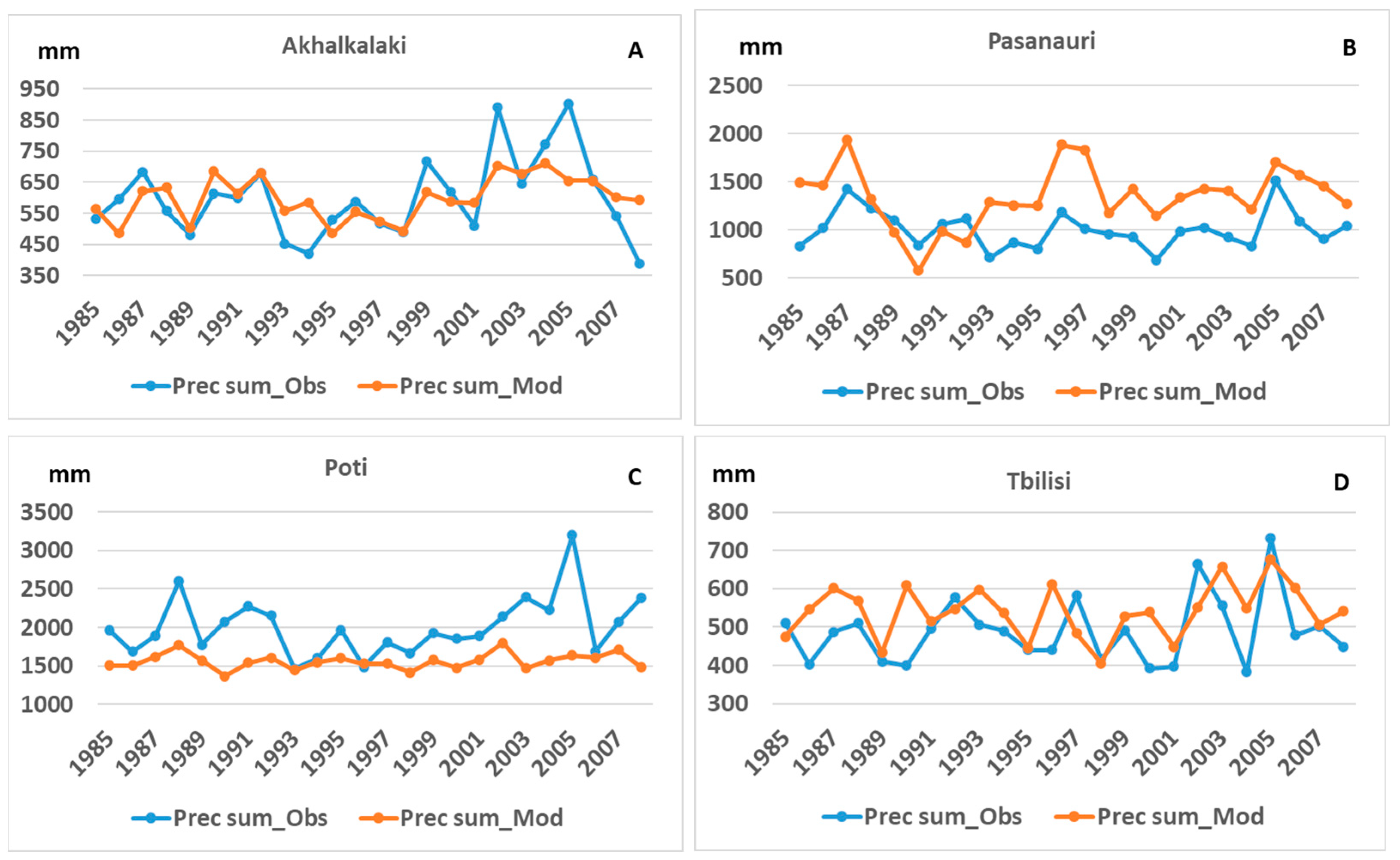
  • The research provides insights into how RegCM4.7.1, using the chosen parameterizations, represents the mean and extreme temperatures and precipitation for the historical period in Georgia.
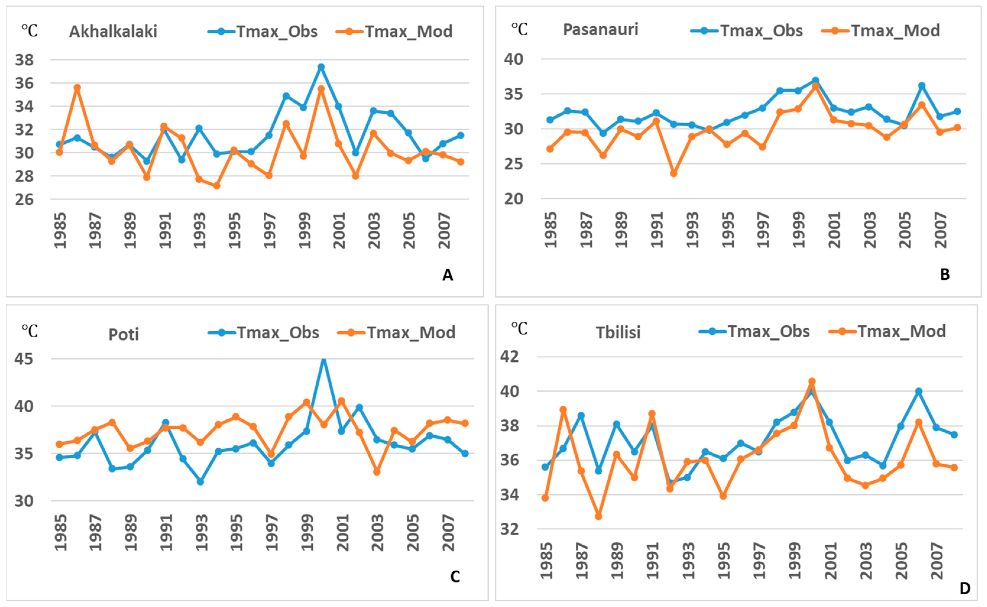
  • The best results when modeling average annual temperatures are obtained for the stations of Gori, Kutaisi, Pasanauri, Tianeti, and Tsalka when the difference between the observation and model data is 0.5 °C or less. Large discrepancies are noted for maximum and minimum temperatures. Overall, the correspondence between the statistical structures of observation and model temperature data can be considered satisfactory.
Observational and model data of the statistical characteristics of annual precipitation sums are often very different. This difference is even greater when modeling the highest and lowest annual precipitation sums. The best results when modeling average annual precipitation are obtained for Akhalkalaki when the difference between observation and model data does not exceed 10 mm.
3.
The correlation between the observational and model data for annual average values, as well as absolute maximum and minimum temperatures, is exceptionally high. For mean annual temperatures, this correlation can be deemed near-perfect, ranging between 0.99 and 1.00.
The correlation for average monthly temperatures is generally high and very high. In the seasonal course of correlation coefficients, the minimum is almost universally observed in July.
In general, the significance level of correlation coefficients for annual and monthly air temperatures is mainly 0.05 and 0.01. In rare cases, the significance level is 0.10, or the relationship is insignificant.
Between annual and seasonal values of precipitation sums, there is generally a moderate correlation (0.5 ≤ R < 0.7), and for precipitation maximums, the correlation is low (0.3 ≤ R < 0.5) and, in some cases, insignificant (0 ≤ R < 0.3).
4.
The bias between the model and observation data is greater for extreme temperatures than for mean temperatures. The bias between the model and observation data is greater for minimum temperatures than for maximum temperatures.
If we consider the difference between the average long-term observation and model data of annual precipitation, then 10 weather stations fall into the −200–200 mm gradation, which is a range close to the natural fluctuation of precipitation, 4 weather stations fall into the 200–400 mm gradation, and 6 weather stations fall into the gradation of 400 mm and more. In general, the results of modeling annual precipitation sums can also be considered satisfactory.
5.
A study of the spatial distribution of bias between actual and model average annual temperatures showed that the greatest fitness between actual and model data was observed at the stations of eastern Georgia (six stations) and Kutaisi. In seven stations, the bias between the observation and model temperatures is positive and falls into the 1.1–3 °C gradation, while on the Black Sea coast stations (Poti, Kobulati, and Zugdidi), the bias is negative, −3–−1.1 °C. The highest bias is in Ambrolauri, and it is in the range of 31.1÷5 °C, while in Dedoplistskaro and Mt. Sabueti, the bias is negative and falls in the range of −5–−3.1 °C.
The smallest bias between the observation and model average annual precipitation was also noted at stations in eastern Georgia, except Tianeti and Pasanauri, located in the Greater Caucasus, as well as Borjomi, where model data are overrated by 200–400 mm. The bias between observation and model average annual precipitation sums is even greater in Ambrolauri and Sachkhere. On the Black Sea coast and the Kolkheti Lowland, the model underestimates the observation data.

Author Contributions

Conceptualization, methodology, writing—original draft preparation, supervision: M.E.; data curation analysis: A.A.; investigation: E.E.; model simulation, visualization: G.M. and T.K.; writing—reviewing and editing: N.C. All authors have read and agreed to the published version of the manuscript.

Funding

This work was supported by the Shota Rustaveli National Science Foundation of Georgia (SRNSFG) grant number: FR-19-8110.

Institutional Review Board Statement

Not applicable.

Informed Consent Statement

Not applicable.

Data Availability Statement

Data are available on request from the corresponding author. The data are not publicly available due to privacy.

Conflicts of Interest

The authors declare no conflicts of interest.

References

  1. Elizbarashvili, M.; Elizbarashvili, E.; Tatishvili, M.; Elizbarashvili, S.; Meskhia, R.; Kutaladze, N.; King, L.; Keggenhoff, I.; Khardziani, T. Georgian climate change under global warming conditions. Ann. Agrar. Sci. 2017, 15, 17–25. [Google Scholar] [CrossRef]
  2. Elizbarashvili, E. Climate of Georgia; Georgian Technical University, Institute of Hydrometeorology: Tbilisi, Georgia, 2017; 360p, Available online: https://www.ecohydmet.ge/geo%20climate.pdf (accessed on 6 March 2024)(In Georgian Language).
  3. Elizbarashvili, E. Climatic Resources of Georgia; Institute of Hydrometeorology: Tbilisi, Georgia, 2007; 321p, Available online: https://www.ecohydmet.ge/saqarTvelos%20klimaturi%20resursebi.pdf (accessed on 6 March 2024)(In Georgian Language).
  4. Keggenhoff, I.; Elizbarashvili, M.; Amiri-Farahani, A.; King, L. Trends in daily temperature and precipitation extremes over Georgia, 1971–2010. Weather Clim. Extrem. 2014, 4, 75–85. [Google Scholar] [CrossRef]
  5. Keggenhoff, I.; Elizbarashvili, M.; King, L. Recent changes in Georgia’s temperature means and extremes: Annual and seasonal trends between 1961 and 2010. Weather Clim. Extremes 2015, 8, 34–45. [Google Scholar] [CrossRef]
  6. Keggenhoff, I.; Elizbarashvili, M.; King, L. Heat Wave Events over Georgia Since 1961: Climatology, Changes and Severity. Climate 2015, 3, 308–328. [Google Scholar] [CrossRef]
  7. Ministry of Environment Protection and Natural Resources of Georgia and UNDP Country Office. Georgia’s Second National Communication to the UNFCCC; Ministry of Environment Protection and Natural Resources of Georgia and UNDP Country Office: Tbilisi, Georgia, 2009. [Google Scholar]
  8. Ministry of Environment and Natural Resources Protection of Georgia. Georgia’s Third National Communication to the UNFCCC; Ministry of Environment and Natural Resources Protection of Georgia: Tbilisi, Georgia, 2015; Available online: https://unfccc.int/sites/default/files/resource/Geonc3.pdf (accessed on 6 March 2024).
  9. Harris, I.; Osborn, T.J.; Jones, P.; Lister, D. Version 4 of the CRU TS monthly high-resolution gridded multivariate climate dataset. Sci. Data 2020, 7, 109. [Google Scholar] [CrossRef]
  10. Harris, I.; Jones, P.D.; Osborn, T.J.; Lister, D.H. Updated high-resolution grids of monthly climatic observations—The CRU TS3.10 Dataset. Int. J. Climatol. 2014, 34, 623–642. [Google Scholar] [CrossRef]
  11. IPCC. The Physical Science Basis. In Contribution of Working Group I of the Fourth Assessment Report of the Intergovernmental Panel on Climate Change; Cambridge University Press: Cambridge, UK, 2007. [Google Scholar]
  12. Kalmár, T.; Pieczka, I.; Pongrácz, R. A sensitivity analysis of the different setups of the RegCM4.5 model for the Carpathian region. Int. J. Climatol. 2021, 41, E1180–E1201. [Google Scholar] [CrossRef]
  13. Valcheva, R.; Popov, I.; Gerganov, N. Convection-Permitting Regional Climate Simulation over Bulgaria: Assessment of Precipitation Statistics. Atmosphere 2023, 14, 1249. [Google Scholar] [CrossRef]
  14. Marinucci, M.R.; Giorgi, F.; Beniston, M.; Wild, M.; Tschuck, P.; Ohmura, A.; Bernasconi, A. High-resolution simulations of January and July climate over the western Alpine region with a nested Regional Modeling system. Theor. Appl. Clim. 1995, 51, 119–138. [Google Scholar] [CrossRef]
  15. Giorgi, F.; Bates, G.T. The climatological skill of a regional model over complex terrain. Mon. Weather Rev. 1989, 117, 2325–2347. [Google Scholar] [CrossRef]
  16. Dickinson, R.E.; Errico, R.M.; Giorgi, F.; Bates, G.T. A regional climate model for the western United States. Clim. Chang. 1989, 15, 383–422. [Google Scholar] [CrossRef]
  17. Giorgi, F.; Marinucci, M.R.; Bates, G.T. Development of a second-generation regional climate model (RegCM2). Part I. Boundary layer and radiative transfer processes. Mon. Weather Rev. 1993, 121, 2794–2813. [Google Scholar] [CrossRef]
  18. Pal, J.S.; Small, E.; Eltahir, E.A.B. Simulation of regional-scale water and energy budgets: Representation of subgrid cloud and precipitation processes within RegCM. J. Geophys. Res. 2000, 105, 29579–29594. [Google Scholar] [CrossRef]
  19. Pal, J.S.; Giorgi, F.; Bi, X.; Elguindi, N.; Solmon, F.; Gao, X.; Rauscher, S.A.; Francisco, R.; Zakey, A.; Winter, J.; et al. Regional Climate Modeling for the Developing World: The ICTP RegCM3 and RegCNET. Bull. Am. Meteorol. Soc. 2007, 88, 1395–1410. [Google Scholar] [CrossRef]
  20. Halenka, T.; Kalvová, J.; Chládová, Z.; Demeterová, A.; Zemánková, K.; Belda, M. On the capability of RegCM to capture extremes in long term regional climate simulation–comparison with the observations for Czech Republic. Theor. Appl. Clim. 2006, 86, 125–145. [Google Scholar] [CrossRef]
  21. Giorgi, F.; Jones, C.; Asrar, G.R. Addressing Climate Information Needs at the Regional Level: The CORDEX Framework. WMO Bull. 2009, 58, 175–183. [Google Scholar]
  22. Gao, X.; Shi, Y.; Giorgi, F. A high-resolution simulation of climate change over China. Sci. China Earth Sci. 2010, 54, 462–472. [Google Scholar] [CrossRef]
  23. Giorgi, F.; Coppola, E.; Solmon, F.; Mariotti, L.; Sylla, M.B.; Bi, X.; Elguindi, N.; Diro, G.T.; Nair, V.; Giuliani, G.; et al. RegCM4: Model description and preliminary tests over multiple CORDEX domains. Clim. Res. 2012, 52, 7–29. [Google Scholar] [CrossRef]
  24. Gutowski, W.J., Jr.; Giorgi, F.; Timbal, B.; Frigon, A.; Jacob, D.; Kang, H.-S.; Raghavan, K.; Lee, B.; Lennard, C.; Nikulin, G.; et al. WCRP COordinated Regional Downscaling EXperiment (CORDEX): A diagnostic MIP for CMIP6. Geosci. Model Dev. 2016, 9, 4087–4095. [Google Scholar] [CrossRef]
  25. Gao, X.; Giorgi, F. Use of the RegCM System over East Asia: Review and Perspectives. Engineering 2017, 3, 766–772. [Google Scholar] [CrossRef]
  26. Boulahfa, I.; ElKharrim, M.; Naoum, M.; Beroho, M.; Batmi, A.; El Halimi, R.; Maâtouk, M.; Aboumaria, K. Assessment of performance of the regional climate model (RegCM4.6) to simulate winter rainfall in the north of Morocco: The case of Tangier-Tétouan-Al-Hociema Region. Heliyon 2023, 9, e17473. [Google Scholar] [CrossRef] [PubMed]
  27. Shi, Y.; Wang, G.; Gao, X. Role of resolution in regional climate change projections over China. Clim. Dyn. 2017, 51, 2375–2396. [Google Scholar] [CrossRef]
  28. Gu, H.; Wang, X. Performance of the RegCM4.6 for High-Resolution Climate and Extreme Simulations over Tibetan Plateau. Atmosphere 2020, 11, 1104. [Google Scholar] [CrossRef]
  29. Holtslag, A.A.M.; Boville, B.A. Local Versus Nonlocal Boundary-Layer Diffusion in a Global Climate Model. J. Clim. 1993, 6, 1825–1842. [Google Scholar] [CrossRef]
  30. Holtslag, A.A.M.; De Bruijn, E.I.F.; Pan, H.-L. A High Resolution Air Mass Transformation Model for Short-Range Weather Forecasting. Mon. Weather. Rev. 1990, 118, 1561–1575. [Google Scholar] [CrossRef]
  31. Zeng, X.; Zhao, M.; Dickinson, R.E. Intercomparison of Bulk Aerodynamic Algorithms for the Computation of Sea Surface Fluxes Using TOGA COARE and TAO Data. J. Clim. 1998, 11, 2628–2644. [Google Scholar] [CrossRef]
  32. Tiedtke, M. A comprehensive mass-flux scheme for cumulus parameterization in large-scale models. Mon. Weather Rev. 1989, 117, 1779–1800. [Google Scholar] [CrossRef]
  33. Federico, S. Implementation of the WSM5 and WSM6 Single Moment Microphysics Scheme into the RAMS Model: Verification for the HyMeX-SOP1. Adv. Meteorol. 2016, 2016, 5094126. [Google Scholar] [CrossRef]
  34. Mielikainen, J.; Huang, B.; Huang, H.L.A.; Goldberg, M.D. Improved GPU/CUDA based parallel weather and research forecast (WRF) Single Moment 5-class (WSM5) cloud microphysics. IEEE J. Sel. Top. Appl. Earth Obs. Remote Sens. 2012, 5, 1256–1265. [Google Scholar] [CrossRef]
  35. Mlawer, E.J.; Taubman, S.J.; Brown, P.D.; Iacono, M.J.; Clough, S.A. Radiative transfer for inhomogeneous atmospheres: RRTM, a validated correlated-k model for the longwave. J. Geophys. Res. Atmos. 1997, 102, 16663–16682. [Google Scholar] [CrossRef]
  36. Ukkonen, P.; Hogan, R.J. Implementation of a machine-learned gas optics parameterization in the ECMWF Integrated Forecasting System: RRTMGP-NN 2.0. Geosci. Model Dev. 2023, 16, 3241–3261. [Google Scholar] [CrossRef]
  37. Oleson, K.W.; Niu, G.; Yang, Z.; Lawrence, D.M.; Thornton, P.E.; Lawrence, P.J.; Stöckli, R.; Dickinson, R.E.; Bonan, G.B.; Levis, S.; et al. Improvements to the Community Land Model and their impact on the hydrological cycle. J. Geophys. Res. Biogeosciences 2008, 113, G01021. [Google Scholar] [CrossRef]
  38. Prein, A.F.; Langhans, W.; Fosser, G.; Ferrone, A.; Ban, N.; Goergen, K.; Keller, M.; Tölle, M.; Gutjahr, O.; Feser, F.; et al. A review on regional convection-permitting climate modeling: Demonstrations, prospects, and challenges. Rev. Geophys. 2015, 53, 323–361. [Google Scholar] [CrossRef] [PubMed]
  39. Coppola, E.; Stocchi, P.; Pichelli, E.; Alavez, J.A.T.; Glazer, R.; Giuliani, G.; Di Sante, F.; Nogherotto, R.; Giorgi, F. Non-Hydrostatic RegCM4 (RegCM4-NH): Model description and case studies over multiple domains. Geosci. Model Dev. 2021, 14, 7705–7723. [Google Scholar] [CrossRef]
  40. Reynolds, R.W.; Rayner, N.A.; Smith, T.M.; Stokes, D.C.; Wang, W. An Improved in Situ and Satellite SST Analysis for Climate. J. Clim. 2002, 15, 1609–1625. [Google Scholar] [CrossRef]
  41. Elizbarashvili, M.; Mikuchadze, G.; Chikhradze, N. Regional Climate Model Simulation of Georgia Precipitation and Surface Air Temperature during 2009–2014. In Proceedings of the International Scientific Conference “Geophysical Processes in the Earth and its Envelopes”, Tbilisi, Georgia, 16–17 November 2023; pp. 166–169. Available online: http://openlibrary.ge/bitstream/123456789/10426/1/40_IG_90.pdf (accessed on 6 March 2024).
  42. Elizbarashvili, M.; Seperteladze, Z.; Mikuchadze, G. The Performance of RegCM4. 7.1 over Georgia’s Territory Using Two Different Configurations. Georgian Geogr. J. 2023, 3, 1–10. [Google Scholar]
  43. Elizbarashvili, M.; Mikuchadze, G.; Kalmár, T.; Pal, J. Comparison of Regional Climate Model Simulations to Observational Data for Georgia. In Proceedings of the EGU General Assembly Conference, EGU23-3828, Vienna, Austria, 23–28 April 2023. [Google Scholar] [CrossRef]
  44. Elizbarashvili, M.; Kalmár, T.; Tsintsadze, M.; Mshvenieradze, T. Regional climate modeling for Georgia with RegCM4.7. In Proceedings of the EGU General Assembly Conference, EGU22-2065, Vienna, Austria, 23–27 May 2022; Available online: https://meetingorganizer.copernicus.org/EGU22/EGU22-2065.html (accessed on 6 March 2024).
  45. Elizbarashvili, M.; Tsintsadze, M.; Mshvenieradze, T. High-resolution Climate Simulation Using Double-nesting Method for Georgia. In Proceedings of the AGU Fall Meeting, New Orleans, LA, USA, 13–17 December 2021; id. A55Q-1638. Available online: https://ui.adsabs.harvard.edu/abs/2021AGUFM.A55Q1638E/abstract (accessed on 6 March 2024).
  46. Bolashvili, N.; Dittmann, A.; King, L.; Neidze, V. (Eds.) National Atlas of Georgia; Franz Steiner Verla: Stuttgart, Germany, 2018; 137p, ISBN 978-3-515-12183-5. [Google Scholar]
  47. Hinkle, D.E.; Wiersma, W.; Jurs, S.G. Applied Statistics for the Behavioral Sciences; Houghton Mifflin Company: Boston, MA, USA, 2003; 756p, ISBN 978-0618124053. [Google Scholar]
  48. Yin Robert, K. Case Study Research Design and Methods, 5th ed.; Sage: Thousand Oaks, CA, USA, 2014; 282p. [Google Scholar]
Figure 1. The topography (m) of the domain for the RegCM4.7.1 simulation and the location of Georgia.
Atmosphere 15 00369 g001
Figure 2. Statistical structure of actual (A) and model data (B) of air temperature by weather stations in 1985–2008.
Atmosphere 15 00369 g002
Figure 3. Statistical structure of actual (A) and model data (B) of atmospheric precipitation according to weather stations in 1985–2008.
Atmosphere 15 00369 g003
Figure 4. Long-term course of observational and model mean annual air temperatures of Akhalkalaki (A), Pasanauri (B), Poti (C), and Tbilisi (D) stations.
Atmosphere 15 00369 g004
Figure 5. Long-term course of observational and model absolute maximum air temperatures of Akhalkalaki (A), Pasanauri (B), Poti (C), and Tbilisi (D) stations.
Atmosphere 15 00369 g005
Figure 6. Long-term course of observational and model absolute minimum air temperatures of Akhalkalaki (A), Pasanauri (B), Poti (C), and Tbilisi (D) stations.
Atmosphere 15 00369 g006
Figure 7. Long-term course of observation and model average annual precipitation amounts of Akhalkalaki (A), Pasanauri (B), Poti (C), and Tbilisi (D) stations.
Atmosphere 15 00369 g007
Figure 8. Annual course of actual and model average monthly air temperatures of Akhalkalaki (A), Pasanauri (B), Poti (C), and Tbilisi (D) stations.
Atmosphere 15 00369 g008
Figure 9. Bias between observation and model average annual temperatures.
Atmosphere 15 00369 g009
Figure 10. Bias between observation and model average annual precipitation sums.
Atmosphere 15 00369 g010
Table 1. Location of meteorological stations according to climatic zones.
NClimate Regions [46] and Weather StationsLocation
Lat, N°Lon, E°Alt, a.s.l., Meter
Maritime humid subtropical climate region.
Excessively humid subzone with prevailing sea breeze during the year and maximum precipitation in autumn–winter.
1.Kobuleti41.8241.783
2.Poti42.1341.704
Maritime humid subtropical climate region.
Humid subzone with well-expressed monsoon-like winds and maximum precipitation in spring–autumn.
3.Kutaisi42.2742.69150
4.Zugdidi42.5241.88117
Maritime humid subtropical climate region.
Sufficiently humid climate with moderate cold winter and comparatively dry hot summer.
5.Zestaponi42.1143.05201
Maritime humid subtropical climate region.
Humid climate with cold winter and prolonged cold summer.
6.Ambrolauri 42.5243.15544
7.Mt. Sabueti 42.0343.481242
8.Sachkhere 42.3543.42415
Moderately humid subtropical climate region.
Moderate warm steppe climate with hot summer and precipitation with two minimums per year.
9.Bolnisi41.4544.55534
Moderately humid subtropical climate region.
Moderate humid climate with moderately cold winter and prolonged warm summer, precipitation with two minimums per year.
10.Borjomi 41.8343.40789
11.Dedoplistskaro41.4746.08800
12.Pasanauri 42.3544.701070
13.Tianeti 42.1244.971099
Moderately humid subtropical climate region.
Transitional climate from moderate warm steppe to moderate humid climate with hot summer and precipitation with two minimums per year.
14.Gori41.9844.12588
15.Sagarejo41.7345.33802
16.Tbilisi41.7244.80403
Moderately humid subtropical climate region.
Moderate humid climate with moderately cold winter and hot summer, precipitation with two minimums per year.
17.Telavi41.9345.48568
Transitional climate subzone from moderately humid subtropical climate to Middle East highland dry subtropic climate.
Highland steppe climate with less snowy cold winter and prolonged cold summer.
18.Akhalkalaki41.4243.481716
19.Akhaltsikhe41.6343.00982
Transitional climate subzone from moderately humid subtropical climate to Middle East highland dry subtropic climate.
Transitional climate from moderately humid climate to highland steppe climate with cold winter and prolonged summer.
20.Tsalka41.6044.081457
Table 2. Correlation coefficients I between actual and model air temperature data.
RegionWeather Station, Altitude a.s.l., mAir TemperatureMonthlyAnnual
JanuaryAprilJulyOctober
Black Sea Coast and Kolkheti LowlandPoti, 3Tmean0.930.890.770.850.99
Tmax0.750.740.840.570.92
Tmin0.650.620.780.640.97
Kutaisi, 114Tmean0.970.940.720.920.99
Tmax0.870.810.450.770.97
Tmin0.680.660.770.630.97
Eastern GeorgiaTbilisi, 403Tmean0.910.960.820.901.00
Tmax0.750.840.780.720.97
Tmin0.770.870.570.710.98
Dedoplistskaro, 800Tmean0.850.940.860.920.99
Tmax0.550.880.690.760.96
Tmin0.650.780.460.670.98
South Georgian HighlandAkhalkalaki, 1716Tmean0.760.910.660.910.99
Tmax0.710.870.310.560.97
Tmin0.610.590.610.660.94
Tsalka, 1457Tmean0.850.970.910.950.99
Tmax0.760.830.480.680.96
Tmin0.550.610.490.470.95
Greater CaucasusPasanauri, 1716Tmean0.900.950.860.920.99
Tmax0.530.750.670.600.96
Tmin0.570.740.580.770.96
Tianeti, 1099Tmean0.820.950.770.910.99
Tmax0.790.810.810.670.97
Tmin0.440.880.500.630.95
Table 3. a and b coefficients for calculating the mean annual air temperature using Formula (1).
Weather StationabWeather Stationab
Akhalki0.877594471.4573585Pasanauri0.924811−2.79561
Akhaltsikhe0.8289770.346824Poti1.0109162.954666
Ambrolauri0.894532−2.15233Sachkhere0.88587−1.00931
Bolnisi0.8495720.560656Sagarejo0.9549861.364985
Borjomi0.862913−0.04571Tbilisi0.9150660.231606
Dedoplistskaro0.9152467294.255145335Telavi0.92004−0.68731
Gori0.88477590.946932Tianeti0.8757651.280343
Kobuleti0.9412223.583432Tsalka0.9284080.971602
Kutaisi0.9924310.540475Zestaponi0.9091090.237966
Mt. Sabueti0.9246194.680622Zugdidi1.0315811.065427
Table 4. Correlation coefficients between actual and model atmospheric precipitation data.
RegionWeather Station, Altitude a.s.l., m PrecipitationCold SpellWarm SpellAnnual
Black Sea Coast and Kolkheti LowlandPoti, 3Sum 0.560.470.59
Max.0.440.140.39
Eastern GeorgiaTbilisi, 403Sum 0.730.520.68
Max.0.500.200.35
South Georgian HighlandAkhalkalaki, 1716Sum 0.560.570.51
Max.0.50.150.23
Greater CaucasusPasanauri, 1716Sum 0.630.550.68
Max.0.420.280.38
Disclaimer/Publisher’s Note: The statements, opinions and data contained in all publications are solely those of the individual author(s) and contributor(s) and not of MDPI and/or the editor(s). MDPI and/or the editor(s) disclaim responsibility for any injury to people or property resulting from any ideas, methods, instructions or products referred to in the content.

