
Time Series Prediction for Energy Consumption of Computer Numerical Control Axes Using Hybrid Machine Learning Models

wbk Institute of Production Science, Karlsruhe Institute of Technology (KIT), Kaiserstraße 12, 76131 Karlsruhe, Germany
*
Author to whom correspondence should be addressed.
Machines 2023, 11(11), 1015; https://doi.org/10.3390/machines11111015
Submission received: 10 October 2023
/
Revised: 28 October 2023
/
Accepted: 31 October 2023
/
Published: 8 November 2023
(This article belongs to the Special Issue Intelligent Machine Tools and Manufacturing Technology)
Abstract
:The prediction of energy-related time series for computer numerical control (CNC) machine tool axes is an essential enabler for the shift towards autonomous and intelligent production. In particular, a precise prediction of energy consumption is needed to determine the environmental impact of a product and the optimization of its production. For this purpose, a novel approach for predicting high-frequency time series of numerically controlled axes based on the program code to be executed is presented. The method involves simulative preprocessing of the input NC code to determine each axis’s acceleration, velocity, and process force. Combined with the material removal rate, these variables are input for a machine learning (ML) model that delivers axis-specific high-frequency time series predictions. Compared to common approaches, it is thus possible to make predictions for the variable energy consumption of machine tools for any tool path or target resolution in the time domain. Experiments show that this approach achieves a high precision when a robust learning data basis is available. For the X-, Y-, and Z-axis, errors of 0.2%, −1.09%, and 0.09% for aircut and of 0.15%, −3.55%, and 0.08% for material removal can be achieved. The potentials for further improvement are identified systematically.
1. Introduction
A reduction in harmful greenhouse gases is necessary to counter climate change and mitigate its consequences. Due to a high energy demand, the manufacturing industry in particular is forced to make conscious and responsible use of its available resources such as energy. This results in ever stricter guidelines, such as the greenhouse gas protocol [1], or extended operating indicators, such as the extended Overall-Equipment-Effectiveness (OEE) OEE+ [2]. Furthermore, steadily rising industrial electricity prices [3] are increasingly motivating companies to reduce their energy consumption. Thus, the incentives for companies to monitor and optimize their energy consumption are constantly increasing.
To adapt and improve energy consumption during or after production, more and more sensors are available during the shift towards Industry 4.0. and digitalization. However, in a highly individualized production, e.g., with a batch size of one, the prediction and the optimization must be carried out before the actual production process. The goal must therefore be to move from a purely reactive adaptation to proactive monitoring and planning.
Most of the manufacturing operations in today’s factories are executed with machine tools. In modern machine tools such as milling machines, machining is performed with the geometrically interpolated movements of computer numerical control (CNC) axes. In combination with the main spindle, these movements transfer the unmachined workpiece into the target geometry through material removal. Thus, the process-dependent energy consumption can be represented using the energy supplied to the axes. The complexity of the movement is strongly dependent on the complexity of the workpiece’s geometry and the planned trajectory. To achieve the highest possible productivity of the machine tools, extremely high dynamics are targeted. In contrast to stationary operations with constant process conditions, the energy supplied is also subject to high fluctuations. Particularly in braking and acceleration processes, this results in short-term but particularly high peaks in consumption. An exact determination of the energy demand and, thus, optimization is only possible by precisely mapping these process details. Thus, a step towards energy-efficient production and optimization is given with the prediction of high-frequency (HF) energy-related time series with a sampling rate above 1 Hz.
2. State of the Art
According to [4], the energy consumers of a machine tool can be subdivided according to the main and auxiliary units. The main units are responsible for the injection of the kinematic energy of all the axes as well as the energy required for material removal. They include the feed axes and the main spindle. The auxiliary units, on the other hand, include all the units that are additionally required for the operation of the machine tool. Depending on the machine, this may include hydraulic units, the cutting fluid supply, or additional cooling systems. The modeling of the entire machine, therefore, consists of the here-considered modeling of the CNC axes as well as the auxiliary units. In the following, publications will be discussed which have the goal of modeling the consumption of the whole machine. Additionally, relevant publications in which the axis-specific energy consumption is to be predicted will be addressed.
Borgia et al. developed [5] a reduced model for the analysis of energy consumption during the milling process. The kinematic quantities were determined and a machine learning (ML) model was trained based on simple motions. In [6], Pavanaskar and McMains developed a tool to determine the machine-specific energy consumption for CNC milling paths based on the material removal rate (MRR). In a validation using linear paths, a deviation between −6% and +5% could be achieved. Edem and Mativenga [7] investigated the parameters influencing the energy consumption of the feed axis during the milling process. A model was derived for a test machine, taking into account the weight of the axes and the workpiece placed on the machine table. During aircut, the model was able to achieve deviations of less than 9%. Based on the results, as well as an investigation of the influence of workpiece and tool orientation on the energy consumption of milling machines [8], Edem and Mativenga [9] developed an extended prediction model. Here, their findings were combined with other models for modeling the overall machine tool consumption. In a simple validation with a small cutting depth (0.5 mm), the model was able to achieve a deviation of −2% with respect to the energy consumption and −4% concerning its machining time. It should be noted, however, that due to the small cutting depth, the influence of the process and, thus, of the axes can be considered rather low. Edem included this finding in his dissertation [10] on modeling the energy demand of machine tool axes and tool paths. Altıntaş [11] studied the modeling and optimization of energy consumption for feature-based milling. A model was developed for estimating the energy requirement, taking into account linear modeling of the axis influence. In a validation, deviations of 5% could be achieved. Furthermore, an investigation of milling strategies for pocket milling using response surface methodology was carried out. To account for the different proportions of total consumption, Zhang et al. [12] developed a multilevel approach to map defined milling conditions. Ma et al. [13] developed a model for a milling process based on the MRR, as well as a model for aircut operations, which could achieve accuracies of >90%. In [14], Imani et al. modeled a machine tool as a thermodynamic system to determine its energy consumption. In a validation, the model was able to achieve a deviation of less than 1%. Simplifications of the model were made. In [15], Lv et al. merged mechanism analysis modeling with a data-driven model to predict the overall consumption of a grinding machine. A support vector machine was used to model the deviation between the actual results and the theoretical model. In a comparison, a pure mechanism model achieved an average deviation of 2.41%, while the data-driven model had an average deviation of 3.13%, and the fused model had an average deviation of 1.98%. Thus, Lv et al. proved the suitability of a combination of mechanism models with data-driven models for the modeling of the complex correlations within machining processes. In [16], Pawar et al. developed a model for circular geometries that achieved deviations below 5%. Yu et al. developed a model for the prediction of energy consumption, as well as the surface quality, when milling stainless steel [17]. In a validation, an accuracy for the prediction of the energy consumption of 98.7% could be achieved. In [18], Brillinger et al. developed an ML-based approach for predicting energy consumption based on the NC code of the part to be produced. Several models were investigated and a deviation of 7.16% was achieved for the whole machine tool system using decision trees. Cao et al. also developed an ML-based prediction of energy consumption [19]. Here, in the first stage, a parser was used to group the NC code, based on which an ML model predicted the energy demand for each state group. This achieved an error per NC block of 5% and an error for the overall program of 0.85%. It can be assumed that the errors in the calculation of the consumption for the entire production balance each other out. In [20], Pawar et al. combined analytical models for the cutting power and empirical ones for the idle speed and auxiliaries to model the energy demand of cam geometries. An error of less than 2.27% could be achieved with this approach. Duc and Trinh [21] developed an approach for the prediction of energy consumption for high-speed milling processes. Here, tool wear was additionally taken into account by calculating the force due to geometry change. In the prediction with a consideration of the wear condition, average errors of less than 9.2% and, without it, less than 18.25% could be achieved. This showed that a consideration of a tool’s condition in the modeling of the energy consumption can lead to better results.
The existing works on modeling the energy consumption of machine tools mostly focuses on a machine level, i.e., they try to model the total energy consumption. Therefore, auxiliary units, as large energy consumers, are primarily responsible for the accuracy of the models. The modeling of the axis-specific energy consumption is only partially addressed. A specific evaluation of the prognosis quality, as in [18], is only rarely the case. By combining the process force with the MRR, a prediction of the process-dependent energy consumption can be made, as shown for example in [13]. However, this is predicted for the overall machine and is not axis-specific. As shown in [15], a combination of analytical and data-based models can be useful. In more recent developments, ML approaches [18,19] are increasingly used for block-wise prediction.
It becomes clear that there is still a need for additional prediction models, especially on an axis level. However, the energy consumption of the axes represents a relevant interface between the machine and the machining process. In the existing works, the prediction of general paths has only marginally been taken into account. In addition, no work is evident in which the prediction of HF time series is directly addressed, which is necessary for a detailed evaluation of the effects of a process’ details and high machine dynamics.
Based on the results presented in the existing works, the following questions can be derived for the present paper:
- How can one predict HF energy-related time series for machine tool axes for general paths, based on the NC code?
- What accuracies can be achieved?
- What are the requirements and limits of the model and how can they be addressed?
3. Approach
The prediction of HF time series based on the NC code is built on three processing steps, as shown in Figure 1. During preprocessing, it is ensured that the existing NC code is given in a standardized form for the subsequent calculations. Thus, the position of the origin of the raw part coordinate system is adjusted if necessary. In a further step, the HF time series of intermediate process variables like time, velocity, acceleration, MMR, and force are simulated. These represent the input for the ML-based prediction of the target time series. The ML model represents the final processing step, mapping the simulated input variables to axis-specific energy-related time series values. The approach aims to make the best possible use of the predictive capabilities of the ML model through simulative preprocessing.
For the training and validation of the machine learning model and the generality of the approach, various datasets were recorded experimentally.
4. Datasets
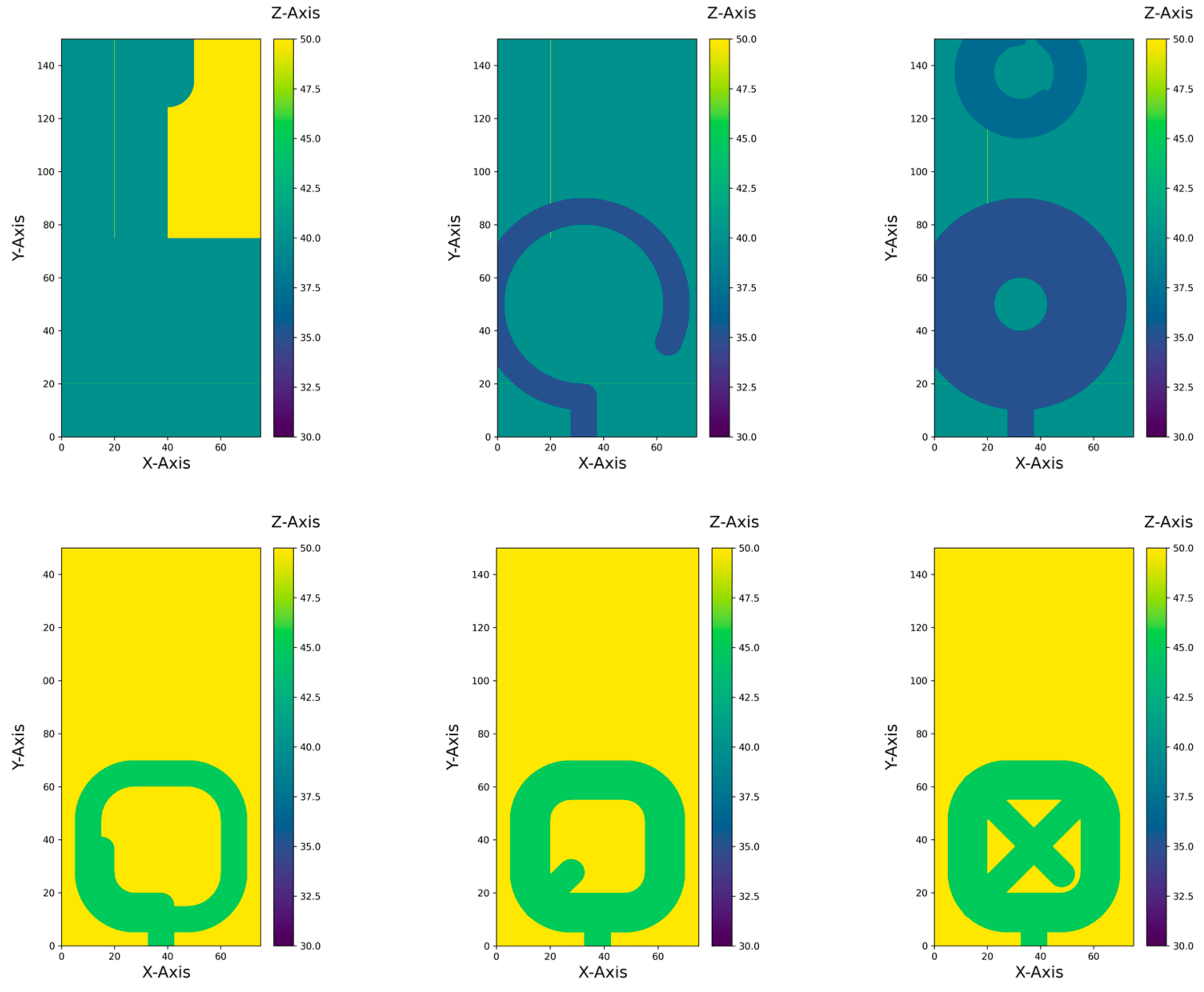
The dataset for the time series prediction in milling processes published in [22] was used for the model development in this publication. The datasets were recorded on a DMG CMX 600 V with a Siemens Industrial Edge and a sampling rate of 500 Hz. Two experimental parts were created for steel (S235JR) and aluminum (2007 T4). Figure 2 shows the tool paths for both parts. Machining was performed using 20 mm, 10 mm, and 5 mm cutters. During the machining process, the feed rate and spindle speed were varied for all the tools to obtain the most comprehensive dataset possible. Furthermore, additional recordings were made without the workpiece (aircut), to be able to specifically investigate the influences of the process forces and, subsequently, the prediction quality.
5. Hybrid Model for HF Time Series Prediction
As described in [23], the milling machine is assumed to be a system of rigid bodies. Due to the equation of motion, the variables acceleration , velocity , and process forces were identified as the primary influences on the energy demand (Equations (1) and (2)) of a given block .
The ML model determines the unknown parameters α, β, and for all the axes . In addition, a strong correlation between the material removal rate and the required power was found in [24]. The MRR is, therefore, used as an additional input variable for the ML model. Considering the MRR, Equation (3) shows all the relevant parts that influence the energy demand due to the model.
The preprocessing NC code simulations are divided into two domains. On the one hand, the kinematic variables are simulated. When aircut predictions should be made, these are the only variables needed. On the other hand, the process variables must be determined. Figure 3 provides an overview of the entire processing steps.
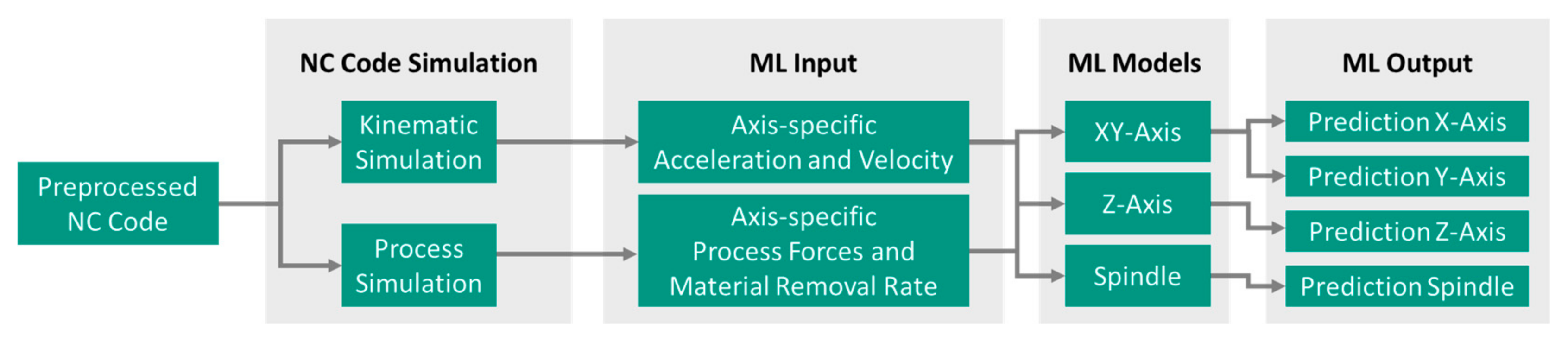
The input variables of the ML model are axis-specific except for the MMR. To achieve the highest possible accuracy, different ML models are used for prediction. Due to the similar characteristics of the X-axis and Y-axis movement during three-axis milling, they are represented using a combined model. The Z-axis and spindle are represented with independent models. The outputs of the ML models are the HF time series for the individual axes. The chosen approach ensures that it can also be trained on other types of signals, such as the torque applied to an axis. Taking into account an acceptable computing time with, simultaneously, a high prediction accuracy, the target frequency is set to 50 Hz.
5.1. Kinematic Simulation
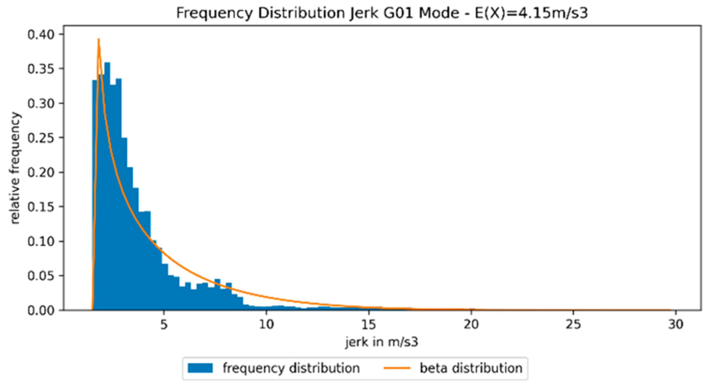
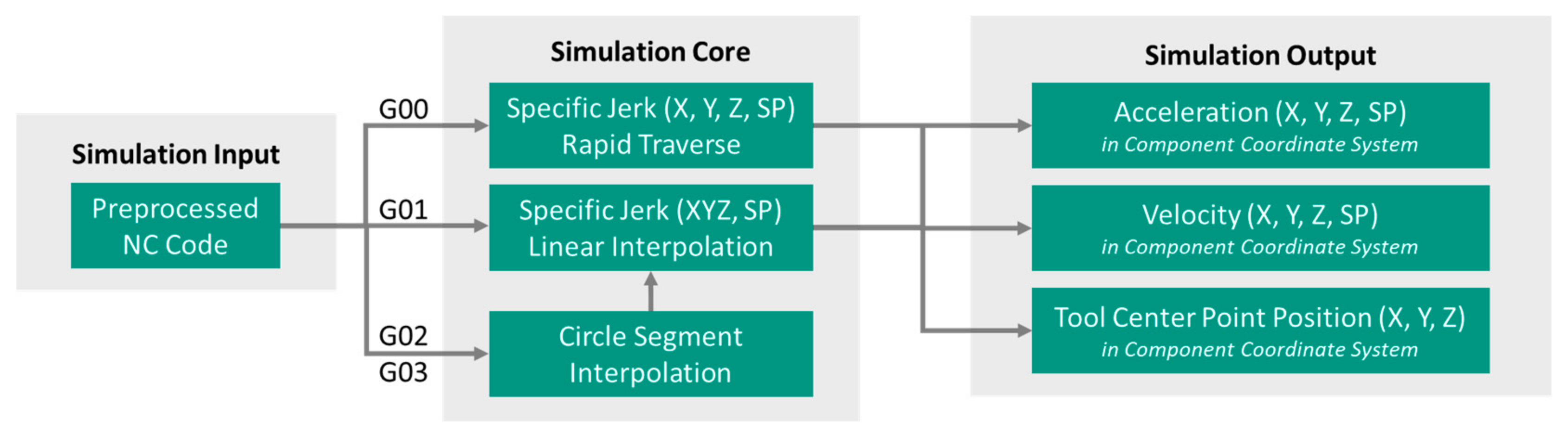
The modeling of the kinematic machine behavior with a machine-specific, characteristic jerk described in [23] is implemented in the kinematic simulations. The simulation can be used to determine the acceleration, velocity, and position of the tool’s center point in the raw part’s coordinate system. A case distinction is made for the machine modes “rapid traverse” (G00) and “linear interpolation” (G01). This is performed because of the different behaviors of the axis. While in the “rapid traverse” mode the axes are moved to the target coordinates as fast as possible, independently, in the “linear interpolation” mode the axes follow a defined path. Therefore, in the “rapid traverse” mode, the machine-specific jerk is determined for each axis individually (X, Y, Z), while, for the “linear interpolation” mode, the machine-specific jerk is determined as the vector addition of the translational axes X, Y, and Z (XYZ). The machine- and case-specific characteristic values for the jerk are determined by building the frequency distributions of large and representative datasets. Figure 4 shows the frequency distribution for the combined jerk of the translational axes (XYZ) for the linear interpolations.
The distribution corresponds approximately to a beta distribution and, thus, can be described by it. The beta distribution with the adjusted function parameters is also shown in Figure 4. The characteristic value searched for the jerk is determined by the expected value of the approximated beta distribution. Using an analogous procedure, the characteristic values for the machine mode “rapid traverse” are determined in an axis-specific way (X, Y, Z) due to the described machine behavior. For circular interpolations, the points on the circle segment are interpolated first. In-between these interpolated points, the sections are connected with linear interpolations.
The kinematic modeling of the spindle (SP) is analogous to the modeling of the translational axes. A machine-specific value for the jerk is equally determined by evaluating the frequency distributions of large datasets. Figure 5 visualizes the kinematic simulation procedure.
5.2. Process Simulation
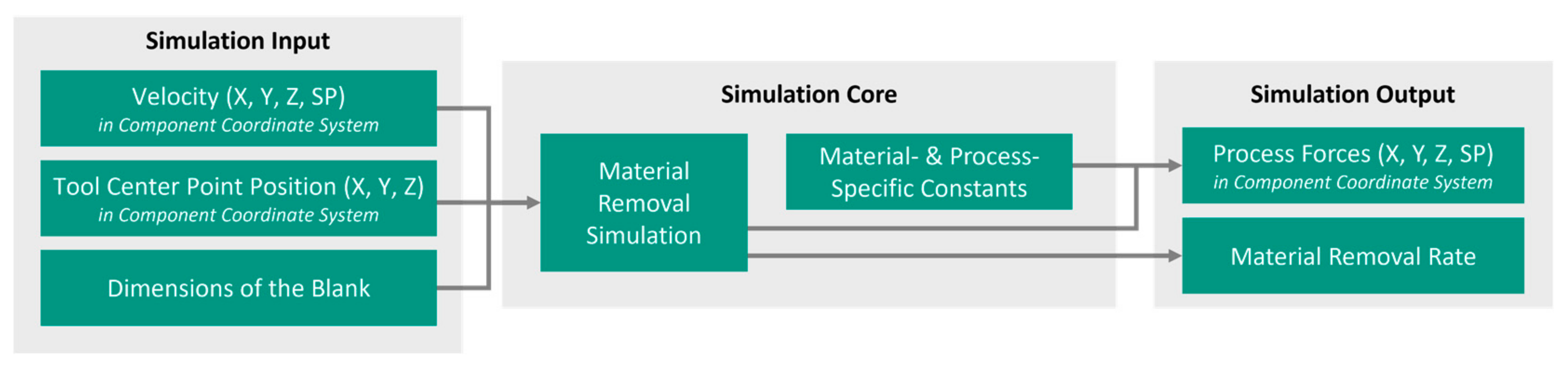
The process simulation aims to determine the ML input variables of the process forces and material removal rate. In the first step, the material removal is simulated. The results of the kinematic simulation for the velocity and position of the tool’s center point are used for this. The dimensions of the raw part are also required for the simulation. A voxel model with a variable resolution is implemented. In the present work, the voxel resolution is set to 0.33 × 0.33 × 1 mm (X × Y × Z). By simulating the path of the milling head, the voxels of the initialized workpiece are reduced in case of overlapping. The model can be used to directly determine the material removal rate. In addition, the removal simulation yields intermediate variables that are required for the process force calculation according to Kienzle’s formulas. These are the tool’s engagement width, tool’s engagement angles, and cutting thickness. Further material- and process-specific variables such as the specific cutting forces, correction factors, or tool diameters must be determined. The literature’s values are used for these specific variables. Figure 6 gives an overview of the process simulation procedure.
5.3. ML Input
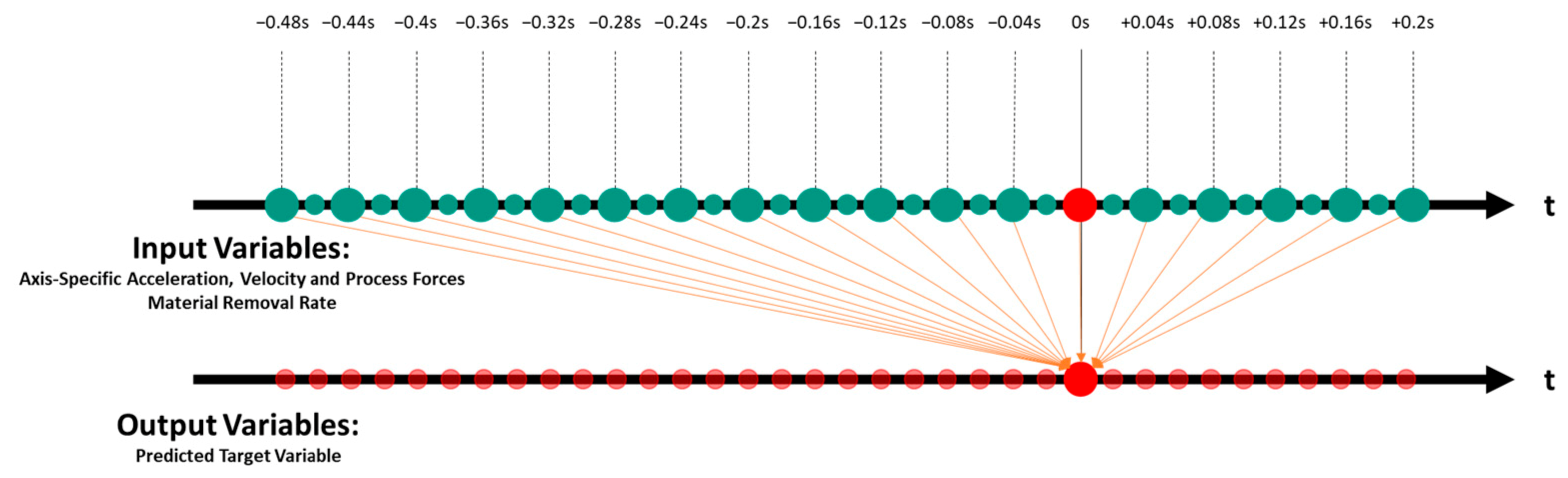
The kinematic and process variables are determined in the raw part’s coordinate system as presented in the previous chapters. Depending on the orientation of the workpiece placed in the machine, a transformation into a machine coordinate system is needed to generate axis-specific input parameters. Thus, the input vector is composed of the speed, acceleration, and force signals of all the axes, as well as the MMR. It is assumed that the system acts with infinite impulse response and that the information processing of the machine tool can take future values into account (look-ahead). For this reason, the values of the last 0.5 and the next 0.2 s should be taken into account. To reduce the amount of data, every second value is used, which leads to a reduced time resolution of 0.04 s or 25 Hz. The resulting scheme can be seen in Figure 7.
Given the input vector with a reduced frequency of 25 Hz (0.04 s intervals), the original time series (500 Hz) of the training datasets must be smoothed accordingly to reduce the HF noises and show the highest possible similarity to the idealized, simulated time series. As the reconstruction of the target signal should be possible, Shanon’s sampling theorem [25] must be fulfilled. Therefore, the original training time series are smoothed in a data preprocessing step using a moving average filter in a neighborhood of 20 past and 20 future datapoints.
5.4. ML Model
Artificial neural feedforward networks with two hidden layers implemented in PyTorch [26] are used for the HF time series predictions. The hidden layers each have the same number of neurons as input variables. The number of input variables is 144 for the aircut predictions and 234 for the predictions considering process forces (see Section 6). ReLUs (rectified linear units) are used as activation functions. The mean absolute error is used as a loss function. The batch sizes are set to 64, 128, or 256. As already described, a total of three models were created for the predictions (XY-axis, Z-axis, spindle).
5.5. ML Output
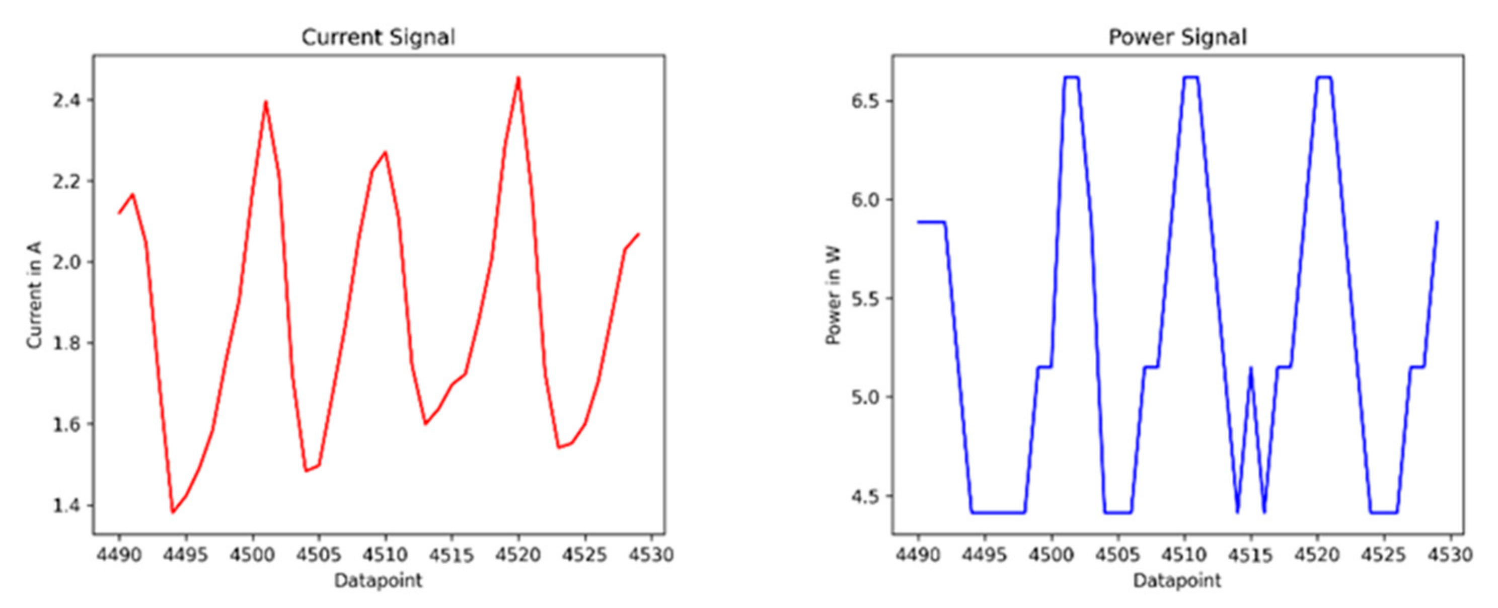
The power signal of the recorded datasets has a low resolution and is strongly discretized due to the measurement technology, as shown in Figure 8. It can also be recognized that there is a strong correlation between the much-higher-resolution current signal and the power signal. A calculation between the variables is possible. The current signal is often used for anomaly detection purposes due to its widespread availability. Therefore, the current signal for the X-, Y-, and Z-axis and the spindle is taken for the prediction. The approach can easily be changed to predict the power signal if a high-resolution power signal is available. By integrating the signal, a prediction can be made regarding the total energy required to execute an NC code. In the present work, the total electric charge is determined as a substitute for the total energy which would be received by integrating a power signal. In this context, the integrated signal serves as a control and evaluation measure.
6. Validation
A total of eight experiments were carried out to validate the approach and the ML models. In four experiments, the predictions for aircuts were evaluated, and, in another four experiments, the process forces were considered. There was a successive increase in the complexity between the individual experiments so that the function, accuracies, and limits of the approach and the ML models could be systematically evaluated. For the experiments, individual learning datasets were specifically combined, and independent validation datasets were formed. The experiments were performed on steel (exp. a) and aluminum (exp. b). The following section gives an overview of the experiments carried out. Experiments 1–4 were executed as aircut experiments, while, in experiments 5–8, tool process forces were present. It must be considered that the datasets for part one are approx. six times more voluminous than the datasets for part two.
6.1. Experiment 1: Training on Part One and Two Aircut Data—Validation on Unseen Data of Part One
For experiment 1, a high characteristic similarity between the learning datasets and validation datasets is chosen. This constellation should provide the best possible dataset for the predictions of the ML models. The aim of experiment 1 is the general verification of the approach and ML models without the consideration of the process forces. This experiment setup corresponds to a classical validation approach with a training data split.
6.2. Experiment 2: Training on Part One Aluminum/Steel Aircut Data—Validation on Part One Steel/Aluminum Data (Exp. a/b)
In experiment 2, different velocity ranges for the axis feed occur in the validation datasets compared to the training datasets. This requires the ML models to perform interpolations and extrapolations. The aim of experiment 2 is to check whether the ML models are able to inter- and extrapolate. This is a first step in checking the generalization capability of the approach.
6.3. Experiment 3: Training on Part One Aircut Data—Validation on Part Two Data
In experiment 3, the characteristics of the training and validation dataset differ. The aim of experiment 3 is to test whether the models are capable of large-scale transfer.
6.4. Experiment 4: Training on Part One and Two Aircut Data—Validation on Unseen Data of Part Two
Experiment 4 is similar to experiment 3, but the training database has been enlarged. The aim of experiment 4 is to investigate how the enlargement of the learning database affects the validation results.
6.5. Experiment 5: Training on Part One and Two Process Data—Validation on Unseen Data of Part One
Experiment 5 represents equivalent investigations to experiment 1, with the difference that the process forces are taken into account. The aim of experiment 5 is the general verification of the approach and the ML models considering the process forces. This experiment setup corresponds to a classical validation approach with a training data split.
6.6. Experiment 6: Training on Part One and Two Process Data—Validation on Unseen Data of Part One
The same data setup is used for experiment 6. By adding a hidden layer, the model complexity of the ML models is slightly increased. The aim of experiment 6 is to test whether small changes in the ML model’s complexity lead to noticeable changes in the prediction results.
6.7. Experiment 7: Training on Part One and Two Process and Aircut Data—Validation on Unseen Part One Data
Experiment 7 has the same setup as experiment 5. Additional aircut data are added to the learning dataset.
6.8. Experiment 8: Training on Part One and Two Process and Aircut Data without Part Two Steel/Aluminum Data—Validation on Part Two Aluminum/Steel Data (Exp. a/b)
Experiment 8 has an enlarged training database in contrast to experiment 7. Compared to experiments 5–7, datasets with comparatively unknown characteristics are used for validation. The aim of experiment 8 is to verify the approach and the ML models in a realistic application.
7. Results
The evaluation of the prediction results was carried out with different evaluation measures. Therefore, the predicted current signals were integrated and compared with the integrated signals of the measurements (total deviation). This was carried out both axis-specific and for the whole process using the sum of all the axes. Furthermore, a dynamic evaluation was carried out using Dynamic Time Warping (DTW). The Python packages dtaidistance [27] and fastdtw [28] were used. With this evaluation method, no absolute statements can be made. However, a direct comparison can be made between the experiments with respect to how well the characteristics of the temporal signal course were predicted. Furthermore, visually comparing the predicted and measured signals provides a good measure for evaluating the results.
Table 1 gives an overview of the total deviations and the DTW-Distances per data point of the experiments. The analysis was carried out on steel (S235JR) for experiment Xa and aluminum (2007 T4) for experiment Xb.
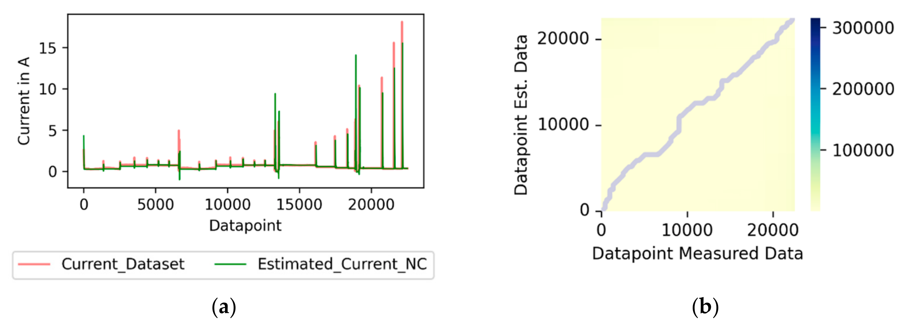
The absolute total deviations for experiment 1 were between 0.09% and 3.74% for the X, Y, and Z-axis. For the spindle, the deviation was slightly higher at −8.83% and −9.51%. Across all the axes, the difference between the predicted and measured values was −0.96% and 0.19%. The visual comparison of the signals showed a high correspondence between the two signals, as Figure 9 shows for experiment 1a as an example of the Y-axis. The relatively linear path through the cost matrix of the analysis via DTW is also shown.
The analysis using DTW confirms that the deviations for the spindle were the highest compared to the other axes, but that they were comparatively much smaller than the integrated deviations, as Table 1 shows. This indicates a good prediction of the characteristics of the spindle with a simultaneous systematic underestimation of the predicted values.
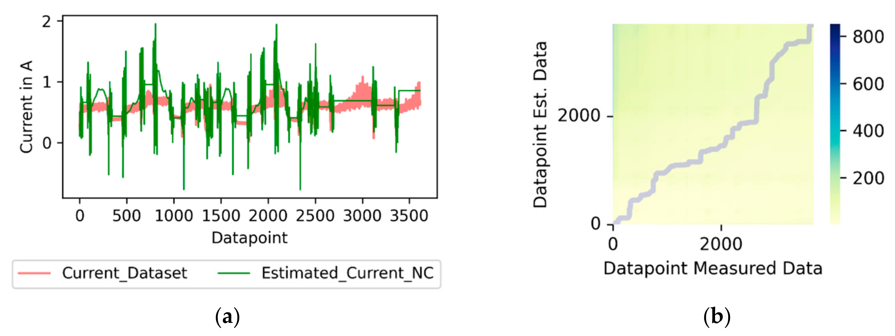
Experiment 2 required the ML model to interpolate and extrapolate through the occurrence of different velocity ranges in the learning and validation data. The total deviations were of the same order of magnitude as in experiment 1, with 1.01% to 2.77% for the X-, Y-, and Z-axis. Comparable deviations to experiment 1 were also achieved for the spindle. The deviations for the evaluation with DTW were in the same order of magnitude as in experiment 1. The characteristics of the prediction were also on the same level as in experiment 1. The results for the spindle are shown in Figure 10.
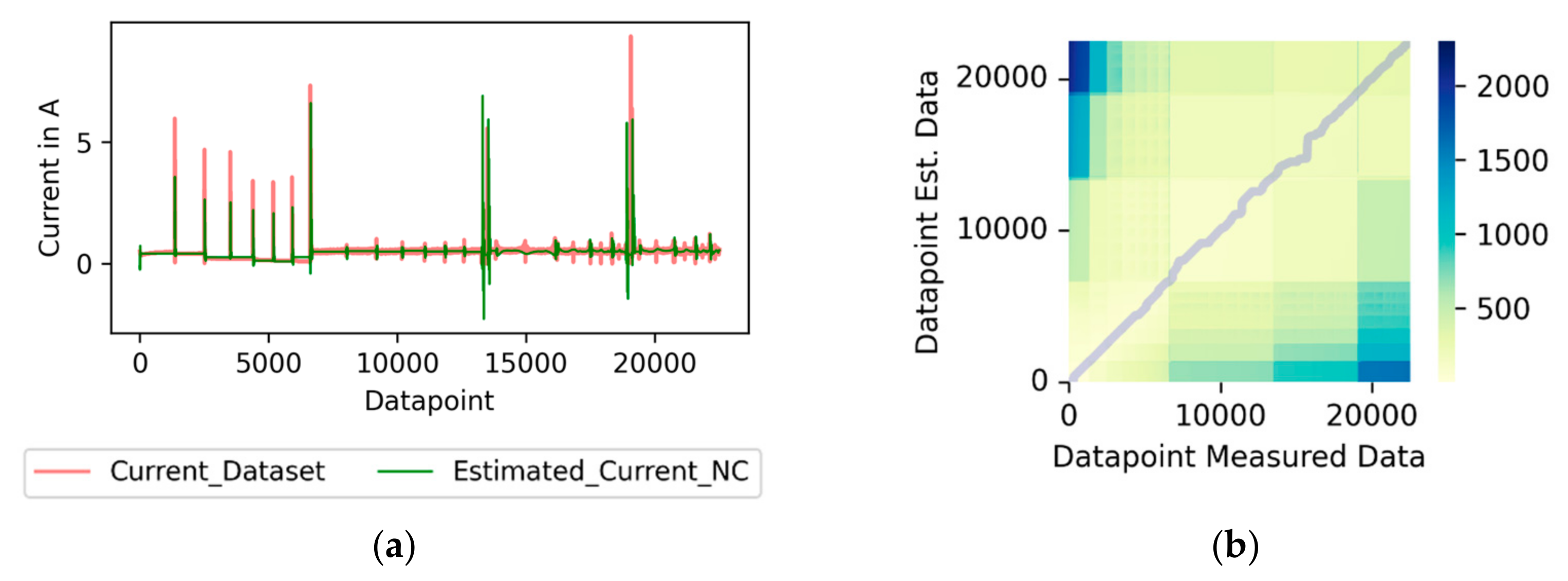
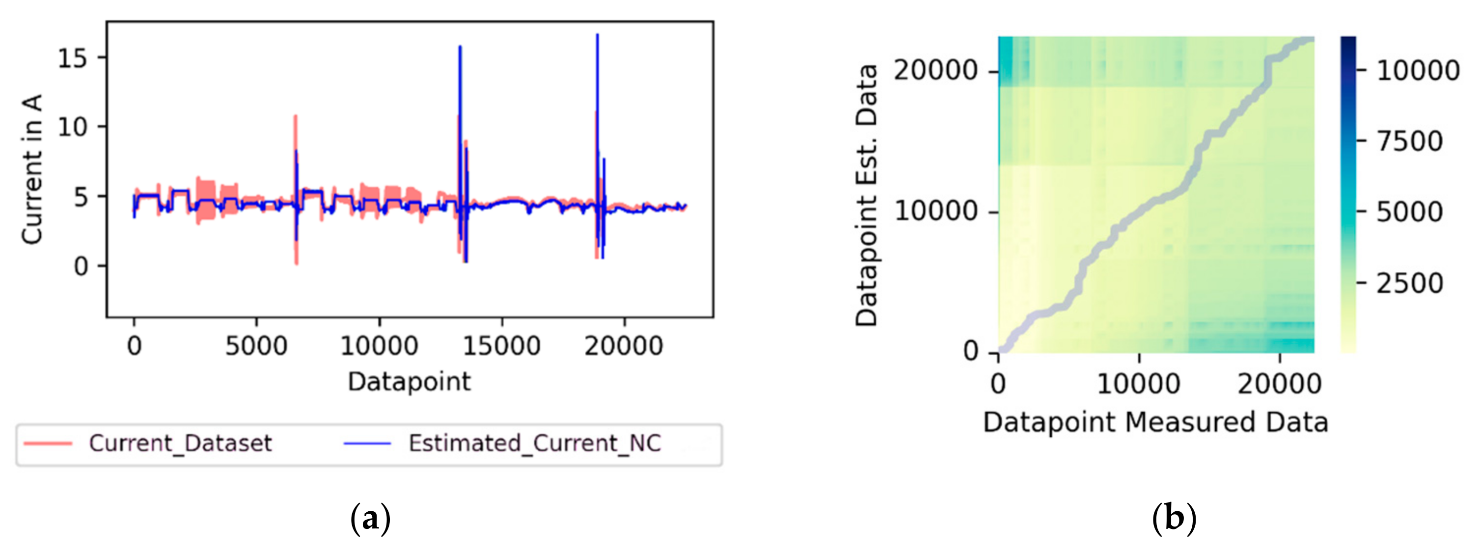
In experiments 3 and 4, the transfer ability of the ML model was investigated. The total deviations in experiment 3 were up to 34.79% higher than in experiments 1 and 2. In experiment 4, the learning dataset was enlarged compared to experiment 3. This was noticeable in the reduced deviations. A maximum total deviation of −2.02% was achieved across all the axes in experiment 4, while this value was 7.38% in experiment 3. Nevertheless, in experiment 4, as in experiment 3, the characteristic of the prediction corresponded only in sections to the characteristic of the measured signal. Figure 11 shows an example of the comparison of the signals for the X-axis in test 4a. Falsely predicted peaks and phase-wise clear deviations in the prediction of the amplitude can be seen. Compared to experiments 1 and 2, the path through the cost matrix is less linear when evaluated using DTW.
The analyses with DTW confirmed the described results of the evaluation using integration, even if the effects were less strong, as Table 1 shows. The deviations across all the axes were smaller in experiment 4, with distances of 864.43 × 10⁻³ and 861.21 × 10⁻³ per datapoint compared to experiment 3, with 991.68 × 10⁻³ and 975.21 × 10⁻³ per datapoint. Nevertheless, the deviations were still higher than the deviations of experiments 1 and 2, with distances between 229.86 × 10⁻³ and 294.91 × 10⁻³ per datapoint.
The results of experiment 5 showed that the approach and the ML model also provided reliable predictions when process forces were taken into account. Figure 12 shows an example of the results of experiment 5a for the Z-axis. To indicate the presence of the process force, blue was chosen for the plot.
Compared to the aircut experiments, it can be seen that the current signal is affected by higher oscillations when the process forces are taken into account. The predicted signal is idealized and exhibits lower oscillations. Furthermore, it can be observed that the deviations in experiment 5 are higher compared to the equivalent aircut experiment 1 (see Table 1). While in experiment 1 the total deviations were consistently in the single-digit percentage area, the deviations of the individual axes in experiment 5 were up to 78.76%. The deviations across all the axes were also higher. The evaluations using DTW showed that the distances per datapoint were an order of magnitude higher in experiment 5 compared to experiment 1.
The comparison of the deviations of experiments 5a and 5b (see Table 1) showed that the predictions for the current amplitude on the material steel (experiment 5a) tended to be underestimated, while the current amplitudes on the material aluminum (experiment 5b) were consistently overestimated. A systematic shift of the deviation ranges for the different materials when evaluated via integration could also be observed for the other predictions considering the process forces (experiments 6–8). Experiment 6 showed that minor adjustments to the model complexity did not change the deviations drastically and led to systematically improved results.
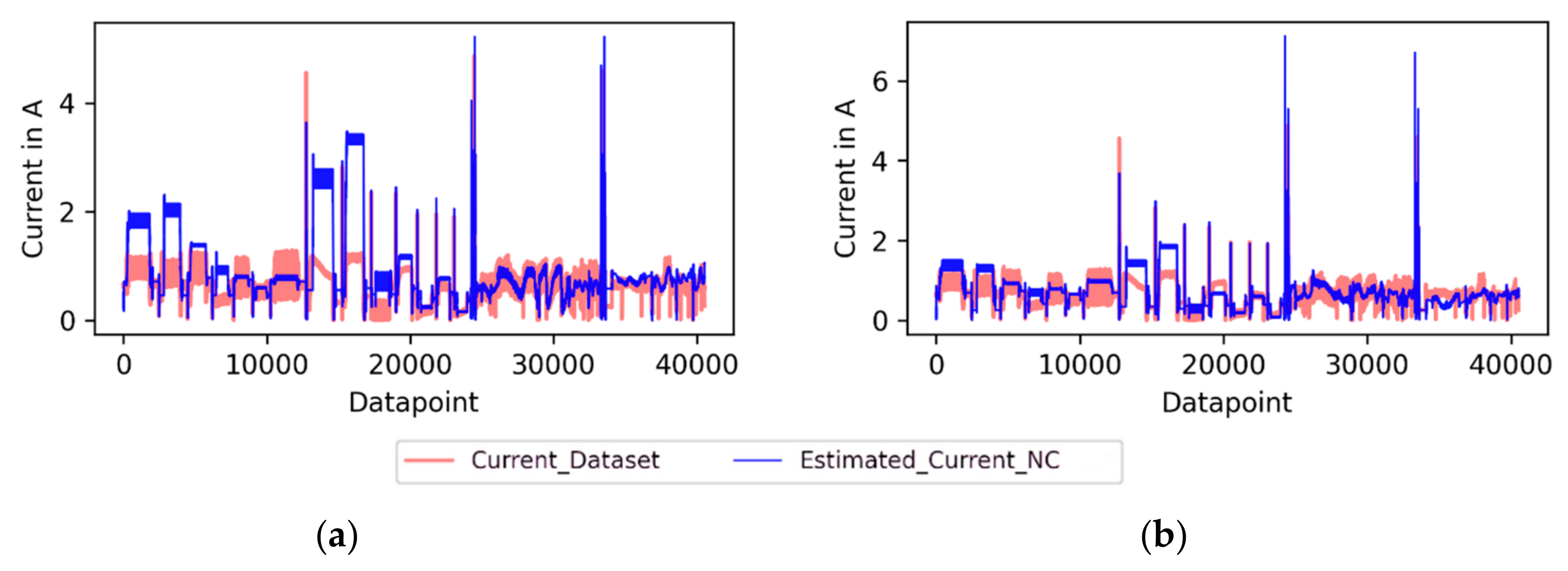
The deviations in experiment 7b were systematically shifted compared to experiment 5b (see Table 1). By adding the aircut training data, the predictions turned out lower overall. Due to the same setup of experiments 5b and 7b, they can be compared directly, as Figure 13 shows exemplarily for the X-axis. It can be observed that the predicted values in experiment 7b are consistently lower compared to experiment 5b. This can be seen particularly well in the area at the beginning. The comparison of all axes also confirms this with a total deviation of 22.95% for experiment 5b compared to 11.45% for experiment 7b.
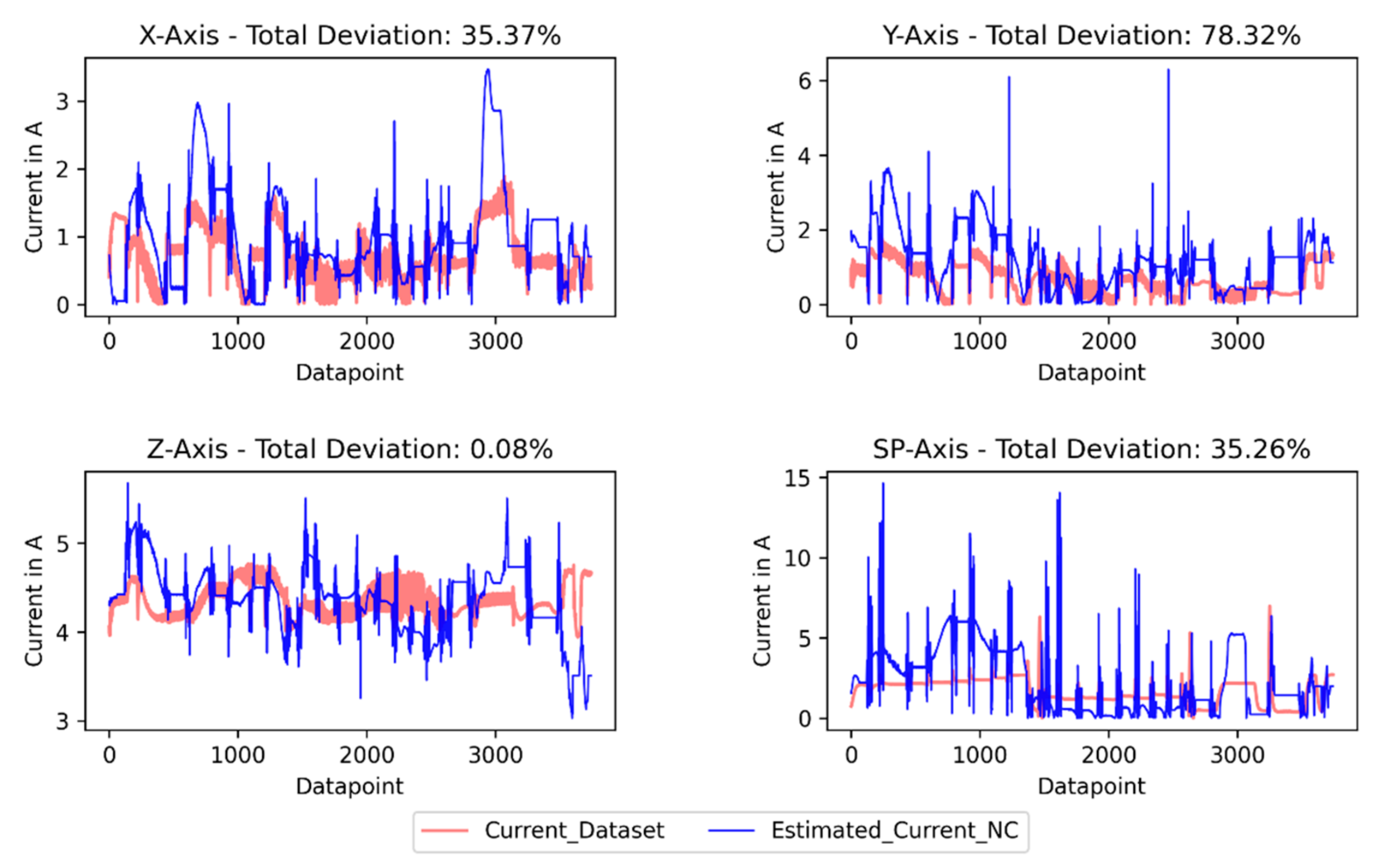
The deviations in experiment 8 were comparatively high, with 35.26% to 169.98% for the X-axis, Y-axis, and spindle. Only the Z-axis deviation was lower, with 0.08% and 2.34%, respectively. Figure 14 shows the results of experiment 8a.
As Figure 14 shows for experiment 8a, the characteristics are not very accurately predicted. Here, it can be seen that the characteristics of the predictions correspond only selectively to the measured values. This is also observed for the Z-axis, where the total deviation is quite small compared to the other axes.
8. Discussion
The kinematic values predicted based on the NC code could be validated by comparing them with the measured values. The temporal deviation of the prediction was low, at 0.33%. The presented approach for kinematic modeling by determining a machine-specific jerk, therefore, appears to be purposeful. The process force simulations could not be validated experimentally. It is, therefore, not possible to estimate the extent to which deviations exist, for example, due to the assumption of material substitution coefficients. However, the simulation of the process forces is only an auxiliary variable on the way to predicting the target time series. The actual criterion for evaluating the model remains the comparison of the output signals (here: current signals). The simulated values for the process forces and material removal rate were used as the training data. The learning data used, thus, represent a hybrid of measured and simulated data. The associated uncertainties affect the ML model and, thus, its predictions.
The prediction results of experiments 1, 2, and 5, in particular, show the potential of the approach and provide a proof of concept. In these experiments, the deviations were small, and the evaluation of the time series showed that the characteristics of the predicted signal matched the measured signal very closely. Experiment 2 shows that interpolations and extrapolations are possible and, thus, validate the generalization potential of the approach. Experiments 3 and 4 show various problems and opportunities. On the one hand, it becomes apparent that, with the datasets available, there could be problems with overfitting, and, thus, that the underlying database is not large enough. This becomes noticeable as the deviations turn out to be higher when learning and validation data are characteristically different. On the other hand, the comparison of the deviations of experiments 3 and 4 shows that a larger data basis leads to considerably improved results. Nevertheless, even the data basis of experiment 4 is not yet sufficient to be considered a generalizable application. When process forces are taken into account, increased deviations usually occur, which is natural due to the additional input variables with a comparatively complex prediction.
For experiment 5, a recurring observation was made that systematically shifted deviation ranges occur for the integrated deviations of the materials steel (experiment a) and aluminum (experiment b). This indicates that the ML model is not able to predict the different materials purely based on the different scales of the simulated forces. Comparable differentiation problems appear in the evaluation of experiment 7. By adding aircut data to the learning datasets, the predictions systematically drop. This is because the amplitudes of the current signals are lower in the aircut data, because of the missing process forces. Thus, the ML model is not able to differentiate adequately whether process forces are present or not and to make a suitably differentiated prediction. Experiment 8 confirms the problems observed in the previous experiments and shows that with the given database and the ML models presented, a generalized application of the approach is not yet possible without accepting high deviations and uncertainties.
The differentiation problems discovered in experiments 5–8, in particular, indicate that the complexity of the artificial neural networks used so far is not enough to be able to deliver precise predictions. If no improvement can be achieved even by using more complex models, the systematic use of case differentiation must be considered. Furthermore, for all the experiments that were carried out considering the process forces, it is shown that the predictions by the ML model show idealized characteristics. The oscillations occurring in the measured values are not represented in the predictions. When evaluating using integration, no systematic deviation occurs due to compensating effects. For the prediction of single values or short time intervals, however, larger deviations can appear. Depending on the purpose of the prediction, this must be considered.
9. Conclusions and Further Work
The present work is dedicated to the prediction of HF energy-related time series of CNC axes based on the program code to be executed. Through the simulative preprocessing of the input NC code, the acceleration, velocity, and process forces are determined for each axis. Together with the simulated material removal rate, these variables form the input for an ML model that provides axis-specific HF time series predictions. The results of the predictions show that the approach used has a high precision if a strong training dataset is given so that the prediction deviations are in the low, single-digit percentage range. Especially, the executed experiments 1, 2, and 5 prove this. The comprehensive investigations also show the existing problems of this model. For example, the learning database should be enlarged, as the comparison of experiments 3 and 4 shows. On the one hand, this can be achieved through the additional, experimental inclusion of machine data. On the other hand, further research should also deal with synthetic learning data generation. In addition, more complex ML models—such as Convolutional Neural Networks, ARIMA, Random Forest, or Gradient Boosting models—should be investigated to further improve the prediction accuracy and address the differentiation problems identified in experiments 5 and 7. The specific analysis of weaknesses of previous predictions for increasing learning efficiency also represents an exciting field of research.
In addition to the mentioned research fields, subsequent works should also focus on possible fields of application. These could particularly address the optimization of energy demand or anomaly detection. Ref. [8] describes that the energy consumption of CNC machine tools is significantly dependent on workpiece and tool path orientation. An implementation of the approach could try to predict the optimal clamping or tool path pose. Furthermore, a high resolution in the time domain allows an optimization of the energy consumption concerning processing details with rapid direction changes. By adjusting the target position specified with the NC code, energy-optimal paths can already be found during path planning. An application in the field of anomaly detection could be the detection of machining irregularities by comparing predicted and measured values.
Author Contributions
Conceptualization, R.S. and Y.P.; methodology, R.S. and Y.P.; software, Y.P.; validation, R.S. and Y.P.; investigation, R.S.; data curation, R.S.; writing—original draft preparation, R.S. and Y.P.; writing—review and editing, S.D.; supervision, J.F. All authors have read and agreed to the published version of the manuscript.
Funding
This Project was supported by the Federal Ministry for Economic Affairs and Climate Action (BMWK), based on a decision by the German Bundestag via Gesellschaft zur Förderung angewandter Informatik e.V.—GFaI. (Grant No. 22849 BG/2).
Data Availability Statement
The training and validation were carried out using the dataset “Training and validation dataset of milling processes for time series prediction” [22], https://doi.org/10.5445/IR/1000157789, last accessed on 15 September 2023.
Conflicts of Interest
The authors declare no conflict of interest.
References
- Bhatia, P.; Ranganathan, J.; World Business Council for Sustainable Development (WBCSD). The Greenhouse Gas Protocol. 2004. Available online: https://www.wri.org/research/greenhouse-gas-protocol-0 (accessed on 7 September 2023).
- Schlagenhauf, T.; Netzer, M.; Fleischer, J. OEE+: Ein Vorschlag zur zeitgemäßen Erweiterung der OEE um Nachhaltigkeitsaspekte= A proposal for the contemporary extension of the OEE to include sustainability aspects. WT Werkstattstech. 2022, 112, 481. [Google Scholar]
- BDEW. (15 February 2023). Industriestrompreise* (Inklusive Stromsteuer) in Deutschland in den Jahren 1998 bis 2023 (In Euro-Cent pro Kilowattstunde) [Graph]. Available online: https://de.statista.com/statistik/daten/studie/252029/umfrage/industriestrompreise-inkl-stromsteuer-in-deutschland/ (accessed on 7 September 2023).
- Denkena, B.; Abele, E.; Brecher, C.; Dittrich, M.A.; Kara, S.; Mori, M. Energy efficient machine tools. CIRP Ann. 2020, 69, 646–667. [Google Scholar] [CrossRef]
- Borgia, S.; Pellegrinelli, S.; Bianchi, G.; Leonesio, M. A reduced model for energy consumption analysis in milling. Procedia CIRP 2014, 17, 529–534. [Google Scholar] [CrossRef]
- Pavanaskar, S.; McMains, S. Machine specific energy consumption analysis for CNC-milling toolpaths. In Proceedings of the International Design Engineering Technical Conferences and Computers and Information in Engineering Conference, Boston, MA, USA, 2–5 August 2015; American Society of Mechanical Engineers: New York, NY, USA, 2015; Volume 57045, p. V01AT02A018. [Google Scholar]
- Edem, I.F.; Mativenga, P.T. Impact of feed axis on electrical energy demand in mechanical machining processes. J. Clean. Prod. 2016, 137, 230–240. [Google Scholar] [CrossRef]
- Edem, I.F.; Mativenga, P.T. Energy demand reduction in milling based on component and toolpath orientations. Procedia Manuf. 2017, 7, 253–261. [Google Scholar] [CrossRef]
- Edem, I.F.; Mativenga, P.T. Modelling of energy demand from computer numerical control (CNC) toolpaths. J. Clean. Prod. 2017, 157, 310–321. [Google Scholar] [CrossRef]
- Edem, I.F. Energy Modelling for Machine Tool Axis and Toolpaths; The University of Manchester: Manchester, UK, 2017. [Google Scholar]
- Altıntaş, R.S.; Kahya, M.; Ünver, H.Ö. Modelling and optimization of energy consumption for feature based milling. Int. J. Adv. Manuf. Technol. 2016, 86, 3345–3363. [Google Scholar] [CrossRef]
- Zhang, C.; Zhou, Z.; Tian, G.; Xie, Y.; Lin, W.; Huang, Z. Energy consumption modeling and prediction of the milling process: A multistage perspective. Proc. Inst. Mech. Eng. Part B J. Eng. Manuf. 2018, 232, 1973–1985. [Google Scholar] [CrossRef]
- Ma, F.; Zhang, H.; Cao, H.; Hon, K.K.B. An energy consumption optimization strategy for CNC milling. Int. J. Adv. Manuf. Technol. 2017, 90, 1715–1726. [Google Scholar] [CrossRef]
- Imani Asrai, R.; Newman, S.T.; Nassehi, A. A mechanistic model of energy consumption in milling. Int. J. Prod. Res. 2018, 56, 642–659. [Google Scholar] [CrossRef]
- Lv, L.; Deng, Z.; Yan, C.; Liu, T.; Wan, L.; Gu, Q. Modelling and analysis for processing energy consumption of mechanism and data integrated machine tool. Int. J. Prod. Res. 2020, 58, 7078–7093. [Google Scholar] [CrossRef]
- Pawar, S.S.; Bera, T.C.; Sangwan, K.S. Modelling of energy consumption for milling of circular geometry. Procedia CIRP 2021, 98, 470–475. [Google Scholar] [CrossRef]
- Yu, S.; Zhao, G.; Li, C.; Xu, S.; Zheng, Z. Prediction models for energy consumption and surface quality in stainless steel milling. Int. J. Adv. Manuf. Technol. 2021, 117, 3777–3792. [Google Scholar] [CrossRef]
- Brillinger, M.; Wuwer, M.; Hadi, M.A.; Haas, F. Energy prediction for CNC machining with machine learning. CIRP J. Manuf. Sci. Technol. 2021, 35, 715–723. [Google Scholar] [CrossRef]
- Cao, J.; Xia, X.; Wang, L.; Zhang, Z.; Liu, X. A Novel CNC Milling Energy Consumption Prediction Method Based on Program Parsing and Parallel Neural Network. Sustainability 2021, 13, 13918. [Google Scholar] [CrossRef]
- Pawar, S.S.; Bera, T.C.; Sangwan, K.S. Energy consumption modelling in milling of variable curved geometry. Int. J. Adv. Manuf. Technol. 2022, 120, 1967–1987. [Google Scholar] [CrossRef]
- Duc, L.A.; Trinh, N.D. A new study for prediction and optimisation of energy consumption during high-speed milling. Int. J. Comput. Integr. Manuf. 2022, 35, 1352–1377. [Google Scholar] [CrossRef]
- Ströbel, R.; Probst, Y.; Fleischer, J. Training and Validation Dataset of Milling Processes for Time Series Prediction; Institut für Produktionstechnik (WBK): Karlsruhe, Germany, 2023. [Google Scholar] [CrossRef]
- Ströbel, R.; Probst, Y.; Hutt, L.; Fleischer, J. Software-Defined Workpiece Positioning for Resource-Optimized Machine Tool Utilization. J. Mach. Eng. 2023, 23, 71–84. [Google Scholar] [CrossRef]
- Diaz, N.; Redelsheimer, E.; Dornfeld, D. Energy Consumption Characterization and Reduction Strategies for Milling Machine Tool Use. In Glocalized Solutions for Sustainability in Manufacturing; Hesselbach, J., Herrmann, C., Eds.; Springer: Berlin/Heidelberg, Germany, 2011. [Google Scholar]
- Shannon, C.E. Communication in the presence of noise. Proc. IRE 1949, 37, 10–21. [Google Scholar] [CrossRef]
- Paszke, A.; Gross, S.; Massa, F.; Lerer, A.; Bradbury, J.; Chanan, G.; Killeen, T.; Lin, Z.; Gimelshein, N.; Antiga, L.; et al. PyTorch: An Imperative Style, High-Performance Deep Learning Library. In Advances in Neural Information Processing Systems 32; Curran Associates, Inc.: Red Hook, NY, USA, 2019; pp. 8024–8035. Available online: http://papers.neurips.cc/paper/9015-pytorch-an-imperative-style-high-performance-deep-learning-library.pdf (accessed on 7 September 2023).
- Meert, W.; Hendrickx, K.; Van Craenendonck, T.; Robberechts, P.; Blockeel, H.; Davis, J. DTAIDistance (v2.3.10). Zenodo. 2020. Available online: https://zenodo.org/records/7158824 (accessed on 7 September 2023).
- Salvador, S.; Chan, P. FastDTW: Toward accurate dynamic time warping in linear time and space. Intell. Data Anal. 2007, 11, 561–580. [Google Scholar] [CrossRef]
Figure 1.
Processing steps of the presented approach.

Figure 2.
Material removal simulation (left to right) for experimental part one (top) and experimental part two (bottom).
Figure 2.
Material removal simulation (left to right) for experimental part one (top) and experimental part two (bottom).

Figure 3.
Information flow from the preprocessed NC code to the axis-specific prediction.

Figure 4.
Frequency distribution for the jerk of the translatory axes (XYZ).

Figure 5.
Flowchart of the kinematic simulation.

Figure 6.
Flowchart of the process simulation.

Figure 7.
Connection scheme of Input and Output Variables.

Figure 8.
Current signal vs. power signal of a sample dataset.

Figure 9.
Results of experiment 1a for the Y-axis with a total deviation of −1.09% in time domain (a) and a DTW-Distance per datapoint of 64.81 × 10⁻³ (b).
Figure 9.
Results of experiment 1a for the Y-axis with a total deviation of −1.09% in time domain (a) and a DTW-Distance per datapoint of 64.81 × 10⁻³ (b).

Figure 10.
Results of experiment 2a for the spindle with a total deviation of −7.66% in time domain (a) and a DTW-Distance per datapoint of 65.76 × 10⁻³ (b).
Figure 10.
Results of experiment 2a for the spindle with a total deviation of −7.66% in time domain (a) and a DTW-Distance per datapoint of 65.76 × 10⁻³ (b).

Figure 11.
Results of experiment 4a for the X-axis with a total deviation of 16.64% in time domain (a) and a DTW-Distance per datapoint of 130.86 × 10⁻³ (b).
Figure 11.
Results of experiment 4a for the X-axis with a total deviation of 16.64% in time domain (a) and a DTW-Distance per datapoint of 130.86 × 10⁻³ (b).

Figure 12.
Results of experiment 5a for the Z-axis with a total deviation of −2.21% in time domain (a) and a DTW-Distance per datapoint of 223.54 × 10⁻³ (b).
Figure 12.
Results of experiment 5a for the Z-axis with a total deviation of −2.21% in time domain (a) and a DTW-Distance per datapoint of 223.54 × 10⁻³ (b).

Figure 13.
Results of experiment 5b for the X-axis with a total deviation of 43.87% in time domain (a) and experiment 7b for the X-axis with a total deviation of 11.48% (b).
Figure 13.
Results of experiment 5b for the X-axis with a total deviation of 43.87% in time domain (a) and experiment 7b for the X-axis with a total deviation of 11.48% (b).

Figure 14.
Results of experiment 8a.


Table 1.
Validation results.
| Experiment | Measure | X-Axis | Y-Axis | Z-Axis | Spindle | All Axes |
|---|---|---|---|---|---|---|
| 1a | Total Deviation | 0.2% | −1.09% | 0.09% | −8.83% | −0.96% |
| DTW-Distance | 69.9 × 10⁻³ | 64.81 × 10⁻³ | 66.96 × 10⁻³ | 93.14 × 10⁻³ | 294.91 × 10⁻³ | |
| 1b | Total Deviation | 2.06% | 3.74% | 0.99% | −9.51% | 0.19% |
| DTW-Distance | 60.22 × 10⁻³ | 71.18 × 10⁻³ | 59.97 × 10⁻³ | 38.49 × 10⁻³ | 229.86 × 10⁻³ | |
| 2a | Total Deviation | −1.59% | −2.77% | 2.25% | −7.66% | 0.44% |
| DTW-Distance | 61.79 × 10⁻³ | 76.17 × 10⁻³ | 86.26 × 10⁻³ | 65.76 × 10⁻³ | 289.98 × 10⁻³ | |
| 2b | Total Deviation | −1.01% | 1.64% | 1.32% | −10.46% | −0.09% |
| DTW-Distance | 67.36 × 10⁻³ | 70.93 × 10⁻³ | 62.4 × 10⁻³ | 59.85 × 10⁻³ | 260.54 × 10⁻³ | |
| 3a | Total Deviation | 33.29% | 16.66% | 8.32% | −34.79% | 7.05% |
| DTW-Distance | 238.97 × 10⁻³ | 197.62 × 10⁻³ | 384.75 × 10⁻³ | 170.34 × 10⁻³ | 991.68 × 10⁻³ | |
| 3b | Total Deviation | 32.46% | 33.89% | 3.63% | −14.9% | 7.38% |
| DTW-Distance | 152.35 × 10⁻³ | 275.81 × 10⁻³ | 335.37 × 10⁻³ | 211.69 × 10⁻³ | 975.21 × 10⁻³ | |
| 4a | Total Deviation | 16.64% | 6.62% | −2.95% | −14.79% | −1.45% |
| DTW-Distance | 130.86 × 10⁻³ | 157.92 × 10⁻³ | 341.87 × 10⁻³ | 233.78 × 10⁻³ | 864.43 × 10⁻³ | |
| 4b | Total Deviation | 15.31% | 6.05% | −4.57% | −7.86% | −2.02% |
| DTW-Distance | 110.69 × 10⁻³ | 167.95 × 10⁻³ | 377.53 × 10⁻³ | 205.03 × 10⁻³ | 861.21 × 10⁻³ | |
| 5a | Total Deviation | 0.15% | −3.55% | −2.21% | −21.55% | −8.11% |
| DTW-Distance | 324.85 × 10⁻³ | 259.92 × 10⁻³ | 223.54 × 10⁻³ | 558.08 × 10⁻³ | 1366.39 × 10−3 | |
| 5b | Total Deviation | 43.87% | 44.17% | 1.45% | 78.76% | 22.95% |
| DTW-Distance | 323.84 × 10⁻³ | 321.22 × 10⁻³ | 226.71 × 10⁻³ | 1154.33 × 10−3 | 2026.10 × 10−3 | |
| 6a | Total Deviation | −1.6% | −5.05% | −3.33% | −24.67% | −9.95% |
| DTW-Distance | 322.65 × 10⁻³ | 270.90 × 10⁻³ | 337.00 × 10⁻³ | 619.26 × 10⁻³ | 1549.81 × 10−3 | |
| 6b | Total Deviation | 43.45% | 43.83% | 1.81% | 69.35% | 21.45% |
| DTW-Distance | 289.60 × 10⁻³ | 311.32 × 10⁻³ | 214.04 × 10⁻³ | 1119.97 × 10−3 | 1934.93 × 10−3 | |
| 7a | Total Deviation | −19.47% | −14.68% | −2.77% | −40.49% | −17.54% |
| DTW-Distance | 395.03 × 10⁻³ | 388.46 × 10⁻³ | 293.08 × 10⁻³ | 1174.27 × 10−3 | 2250.84 × 10−3 | |
| 7b | Total Deviation | 11.48% | 36.73% | −0.11% | 40.26% | 11.45% |
| DTW-Distance | 168.99 × 10⁻³ | 270.81 × 10⁻³ | 145.81 × 10⁻³ | 599.64 × 10⁻³ | 1185.25 × 10−3 | |
| 8a | Total Deviation | 35.37% | 78.32% | 0.08% | 35.26% | 18.49% |
| DTW-Distance | 356.31 × 10⁻³ | 382.32 × 10⁻³ | 203.73 × 10⁻³ | 897.44 × 10⁻³ | 1839.8 × 10−3 | |
| 8b | Total Deviation | 68.44% | 106.61% | 2.34% | 169.98% | 41.45% |
| DTW-Distance | 349.48 × 10⁻³ | 624.84 × 10⁻³ | 176.59 × 10⁻³ | 787.27 × 10⁻³ | 1938.19 × 10−3 |
Disclaimer/Publisher’s Note: The statements, opinions and data contained in all publications are solely those of the individual author(s) and contributor(s) and not of MDPI and/or the editor(s). MDPI and/or the editor(s) disclaim responsibility for any injury to people or property resulting from any ideas, methods, instructions or products referred to in the content. |
© 2023 by the authors. Licensee MDPI, Basel, Switzerland. This article is an open access article distributed under the terms and conditions of the Creative Commons Attribution (CC BY) license (https://creativecommons.org/licenses/by/4.0/).
Share and Cite
MDPI and ACS Style
Ströbel, R.; Probst, Y.; Deucker, S.; Fleischer, J. Time Series Prediction for Energy Consumption of Computer Numerical Control Axes Using Hybrid Machine Learning Models. Machines 2023, 11, 1015. https://doi.org/10.3390/machines11111015
AMA Style
Ströbel R, Probst Y, Deucker S, Fleischer J. Time Series Prediction for Energy Consumption of Computer Numerical Control Axes Using Hybrid Machine Learning Models. Machines. 2023; 11(11):1015. https://doi.org/10.3390/machines11111015
Chicago/Turabian StyleStröbel, Robin, Yannik Probst, Samuel Deucker, and Jürgen Fleischer. 2023. "Time Series Prediction for Energy Consumption of Computer Numerical Control Axes Using Hybrid Machine Learning Models" Machines 11, no. 11: 1015. https://doi.org/10.3390/machines11111015
Note that from the first issue of 2016, this journal uses article numbers instead of page numbers. See further details here.