Abstract
A multi-branch pipeline is a typical structure, which is widely used in aerospace, marine and other hydraulic systems. The multi-branch pipeline suffers serious vibration from fluid–structure interaction, which can cause vibration failures in the pipeline system through overload in engineering fields. Vibrational analysis of the multi-branch pipeline system is increasing as part of the design of hydraulic system. In this paper, the finite element model of a multi-branch pipeline considering fluid—structure interaction is established, and the effectiveness of the modeling is validated through a comparison of the modal test for a typical four-way pipeline. The effects of the flow rate, pressure, fluid medium, pipe diameter, elastic constraint stiffness, and pipeline length and wall thickness on the dynamic characteristics of pipeline system are all considered. The obtained results indicate that the multi-branch junction suffering from significant vortex fluid is the main cause of fluid-induced vibration of the pipeline system. The fluid and structural parameters have great influence on the vibration characteristics of the pipeline, which can serve as an efficient tool in the design and maintenance of multi-branch hydraulic pipeline systems.
1. Introduction
A multi-branch pipeline is a typical structure, consisting of a straight pipe, nut, rear ferrule, front ferrule and four parts of the joint body. It is widely used in aerospace, shipbuilding and other fields, with the advantages of small size and convenient operation. The pipeline suffers serious vibration from fluid-structure interaction, and long-term vibration will reduce the life of the pipeline and hydraulic components, and in serious cases may even cause wall rupture and damage to the pipeline support structure. It causes loss of support stiffness, piping system failure, and joint leakage [1,2,3]. Therefore, it is urgent to study the vibration behavior of pipeline to reveal the influence mechanisms of various parameters on its vibration behavior.
The fluid-structure interaction mechanism is defined as three kinds of coupling [4,5,6]. Poisson coupling is due to the Poisson effect, in which the oscillating pressure causes the radial pipe wall to expand, resulting in axial strain and movement. Due to the unbalanced pressure acting on a certain area, the coupling of the joint occurs at the boundary of change, such as elbow, valve, joint and pipe end. Friction coupling is caused by the shear stress on the pipe wall and is generally considered less important than the other two couplings. To describe the vibration characteristics of pipelines, several models are proposed according to basic equations. Ouyang et al. [7,8] considered the stress distribution around the section perpendicular to the axis of the hydraulic pipe according to the two-dimensional model, taking into account the effects of curvature and stress concentration. On the basis of the characteristic line method, the vibration characteristics of a simple straight pipe were accurately predicted by using the eight-equation model, and on this basis, the effects of curvature and friction on the resonance frequency of the pipe section were analyzed. Andrade et al. [9] developed a quasi-two-dimensional flow model for fluid transport in pipes, analyzed the energy transfer and dissipation effects in fluid piping systems, effectively described frictional coupling, and accurately captured energy dissipation in fluids. Zhang, Quan et al. [10,11] used the 14-equation fluid-structure interaction vibration model of hydraulic pipe. The accuracy of the FSI frequency domain solution at high Reynolds number is improved and the accuracy of the friction coupling model analysis is verified. Bai et al. [12] established a new dynamic model for the cantilever pipe conveying variable density fluid in combination with the Bernoulli-Euler beam model. The results showed that the pipeline system is prone to losing stability when the fluid density increases. Gao et al. [13,14,15] analyzed the research status of aviation hydraulic pipeline vibration and control technology in the field. A model reduction method was developed, and artificial springs were introduced to simulate boundary conditions, which significantly reduced the computational cost of the vibration analysis of long-distance multi-elastically supported hydraulic pipelines. Tan, Chai et al. [16,17,18] established a nonlinear coupling dynamic model of the flow conveying pipeline based on the Timoshenko beam and verified the accuracy of the model through the finite difference method (FDM). The results showed that the Timoshenko model was more accurate in analyzing large flow rate, amplitude or short pipeline length. Yuan et al. [19,20] developed a novel finite element model based on the absolute nodal coordinate formula (ANCF) and a dynamic mechanical model based on the Timoshenko beam theory for curved pipes conveying fluid, and analyzed the vibration characteristics of curved pipes under the influence of the fluid flow. Then, through the finite element numerical simulation, they verified the accuracy of the model.
On the basis of the model equations, the following researchers have investigated the fluid–structure interaction of pipelines using different calculation methods. Wiggert et al. [21,22,23] used the characteristic line method to carry out research on pipeline system vibration for many years. They then put forward a mathematical model describing the fluid–structure interaction of a liquid-filled pipeline and carried out modal analysis of a liquid-filled pipeline system through the transfer matrix method. Dai et al. [24] studied the influence of the combined force caused by fluid flow on the natural frequency of straight pipes and elbows by using the transfer matrix method. When analyzing the vibration of pipes containing flowing fluid, the stable resultant force generated by fluid flow must be considered. Kalliontzis [25] realized accurate FSI calculation under the structural response dominated by axial, bending and shear motion through the ALE formula, and verified the accuracy of the method using existing commercial software. Huang et al. [26] used the element-free Galerkin method to calculate the natural frequencies of the two ends of the straight pipe under different boundary conditions and obtained the natural frequency equations of the fluid transmission pipeline under different boundary conditions. Zhu et al. [27] used fluid dynamics (CFD) and fluid–structure interaction calculation methods to obtain the flow characteristics of the oil flow, and analyzed the effect of the diameter ratio of the branch pipe to the straight pipe in the T-pipe and the merging angle of the three branches on the flow and deformation of the pipe. Francis [28] proposed a complete Lagrangian finite element method (FEM) with node integration to simulate the fluid–structure interaction problem. The accuracy of the method was proved through experimental tests, providing a reference for solving complex FSI problems. Lavooij, Wang et al. [29,30] used the finite element method combined with the characteristic line method (MOC-FEM) to solve the pipe equations based on the characteristic line method. The transient analysis of the fluid-filled pipeline was completed, which significantly improved the calculation efficiency of the coupled vibration of the hydraulic pipeline system. Liu et al. [31] developed the transfer matrix method for vibration analysis of branch pipes to compare the calculated pressure frequency response of rigid pipes and flexible pipes. This method was easier to use and can be used to calculate branch pipes with different shapes. Based on the fluid-structure interaction, Wu et al. [32,33] used the structural and fluid-dynamic models to analyze the fluid-structure coupling vibration of the pipeline, as well as analyzing the pipeline vibration response under different working conditions, providing a reference for practical engineering application.
The research on the fluid-structure interaction vibration characteristics of pipelines has already yielded a wealth of results. Different mathematical theoretical models have been established for straight pipes, elbows, T-shaped pipes, etc. The pipeline vibration has been analyzed using the characteristic line method, transfer matrix method, and finite element method, etc. However, there are few literature reports on the multi-branch pipeline, so it is necessary to explain the law of fluid in the multi-branch pipeline. Compared with other types of pipes, the fluid changes acutely when flowing in the multi-branch pipeline, especially at the junction. Where the fluid collides with the wall to generate eddy current, the influence of the fluid-structure interaction on the pipeline is significantly increased. Therefore, the finite element model of a multi-branch pipeline is established, and the influence of different parameters on the vibration characteristics of the pipeline is analyzed, providing a reference for the subsequent structural optimization design.
2. Finite Element Analysis and Equation of Motion for Pipeline System
2.1. Finite Element Model of the Pipeline System
The pipeline system composed of a typical ferrule type hydraulic four-way joint is considered. The ferrule type joint is composed of four parts: nut, front ferrule, rear ferrule and joint body. The schematic diagram of the pipeline is shown in Figure 1. The mechanical properties of pipeline system are shown in Table 1. The inner diameter of the pipeline is 10 mm, the wall thickness of the pipeline is 1 mm. Each length of the pipeline is 250 mm, A is for the inlet, and B, C, D are for the outlet.
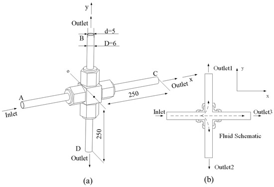
Figure 1.
Schematic diagram of the multi-branch pipeline. (a) Front view of model. (b) Model section view.

Table 1.
Mechanical properties of pipeline system.
2.2. Equation of Motion for Fluid–Structure Interaction
2.2.1. Equation of Fluid Motion
The fluid motion in the pipeline is regarded as incompressible flow. The fluid continuity equation is from [33]:
The momentum equation is
where ρ, μ, k, u, and are the fluid density, dynamic viscosity of the fluid, turbulent kinetic energy, averaged velocity component, and Reynolds stress component, respectively. Herein, δ is the “kroneckerdelta” symbol, and the subscript i and j represent the time. If the subscript i is equal to j, δij is one, otherwise δij is zero.
The standard k-ε turbulent equation is used to express the fluid motion state in the pipeline, which is expressed as
where Gk, Gb, YM, C*1ε, and C2ε are the terms for the generation of turbulent kinetic energy due to the mean velocity gradient turbulent dissipation rate, the generation of turbulent kinetic energy due to the influence of buoyancy, correction coefficient, empirical constant, Prandtl numbers corresponding to turbulent kinetic energy and dissipation rate, respectively. The subscripts k, ε, and t represent turbulent kinetic energy, dissipation rate, and time, respectively.
2.2.2. Equation of Pipeline Motion
The equation of motion for the pipeline system with n degrees of freedom is expressed as in [34]:
where MG, CG, KG, q, fo, and Fd are the global mass matrix, damping matrix, stiffness matrix of the pipeline, displacement vector, vector of fluid–structure interaction forces at the fluid solid interface, and external excitation vector except fluid-structure interaction, respectively.
2.2.3. Equation of Motion for the Pipeline with Fluid-Structure Interaction
Figure 2 shows the schematic diagram of the force and displacement transfer relationship between the pipeline and fluid at the interface. Fluid-structure interaction occurs at the interface between fluid and pipe structure, where the physical quantity is transferred. The normal velocity (v) continuity, normal stress (τ) continuity, and displacement (x) continuity are expressed as
where the subscripts f and s represent the fluid and solid domain side at the fluid–solid interface, respectively.
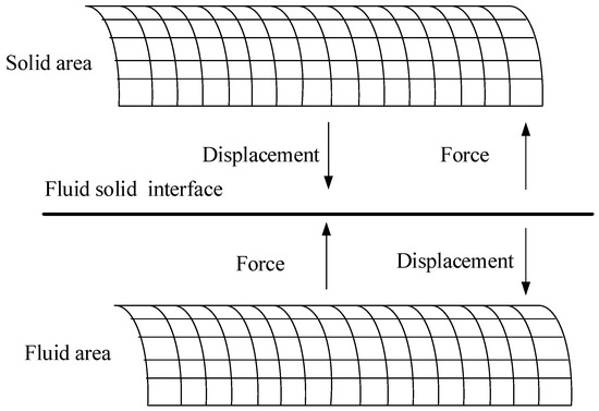
Figure 2.
Schematic diagram of fluid–solid interface.
3. Experimental Verification on the Inherent Characteristics of the Pipeline
3.1. Modal Analysis on the Pipeline without Fluid
Figure 3 shows the schematic diagram for modal analysis on the empty pipe. Four sections of pipeline are connected with a ferrule type four-way joint. Each end of the pipeline is fixed on the vibration test bench with brackets. The pipeline system is excited at the points marked in advance by an impact hammer (PCB, model 086C01), vibration responses are measured by accelerometers (PCB, model 352C22).
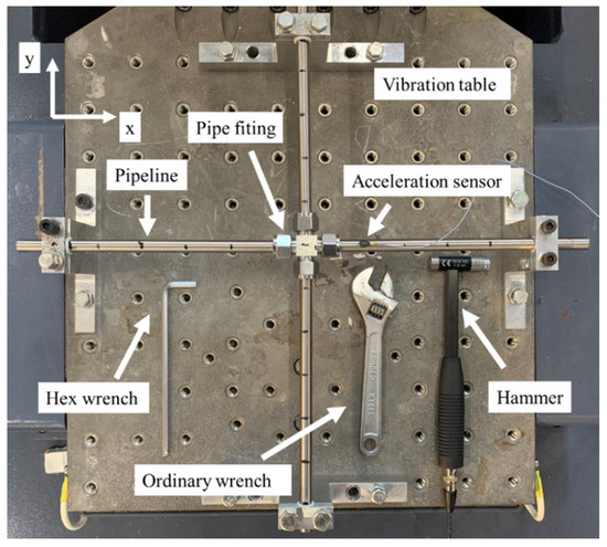
Figure 3.
Schematic diagram of empty pipe modal test.
For the simulation analysis of hollow pipe modal and frequency response, the pipe section is divided by a hexahedral mesh of 2 mm in size. The joint and nut are divided by tetrahedral mesh of 4 mm in size, and the pipe is fixed and supported at all four ends. The results of the natural frequency obtained from the pipeline simulation and experiment are shown in Table 2. Figure 4 shows the comparison of FRF from the experiment and simulation. The simulation of the first three orders of natural frequency of the pipeline system match with the experimental results, the maximum error is under 7%, and the corresponding vibration pattern is shown in Figure 5. The reasons for that discrepancy include the accuracy of the instrument, the processing error of the pipeline, and the simplification of the four-way joint by the finite element model. Moreover, the acceleration sensor could add a small quantity of mass, and the additional mass of the longer part of the pipeline is not considered. Generally speaking, the experimental and the numerical results are in good agreement and, therefore, the accuracy of the proposed methodology was verified.
Table 2.
Comparison of natural frequency of empty pipe.
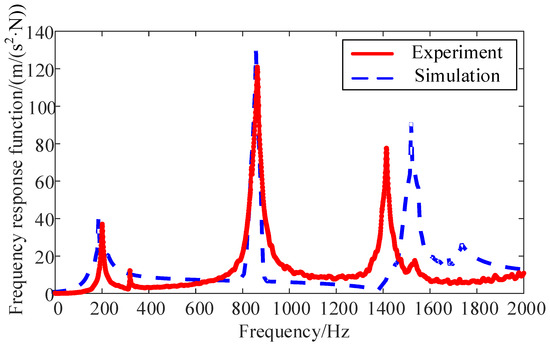
Figure 4.
Comparison of frequency response function between experiment and simulation.
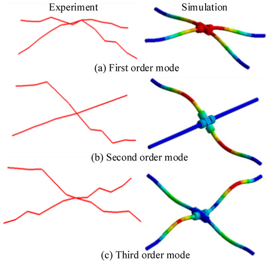
Figure 5.
Comparison of empty tube experiment and simulation mode shape.
Figure 5 shows the first three vibration bending modes of the pipeline. The first-order vibration mode is the overall bending vibration of the pipeline centered on the joint. The second-order vibration mode is the bending vibration of two pipes with the same axis symmetrical to the joint. The third-order mode of vibration is the bending vibration of four pipes symmetrically with a joint.
3.2. Modal Analysis on the Pipeline Filled with Fluid
Modal analysis on the pipeline filled with fluid is carried out, and the experiment schematic is shown in Figure 6. The hydraulic hoses are connected with fittings on both sides of the x-axis as shown in Figure 3, the other directional branch pipe is plugged with plugs.
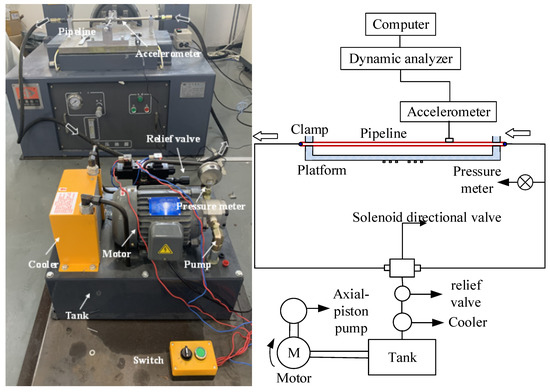
Figure 6.
Schematic diagram of liquid-filled pipeline experiment.
The simulation analysis of the liquid-filled pipeline is carried out. As the flow rate of the pump is 1.5 L/min, the flow rate and inlet pressure in the pipeline are calculated to be 0.3 m/s and 2 MPa, respectively. After the simulation, the results are transmitted to the mechanical module as pressure loads for the pre-stress modal analysis and frequency response analysis. As the coupling effect of the liquid and pipeline should be considered, hydraulic oil is equivalent to incompressible metal material with the same density. The bulk modulus is 160 MPa, and Poisson’s ratio is zero. The hydraulic oil is simulated with solid units. The contact between the pipe and the support is bonded, and the constraint between the hydraulic oil and the inner wall of the pipe shows no separation, respectively. The liquid material parameters are shown in Table 3.
Table 3.
The properties of the liquid.
The comparison of the dynamic characteristics of the experiment and simulation is shown in Table 4 and Figure 7. The first three orders of natural frequency of the piping system from the experiment and simulation are similar, and the maximum error is under 6%. This is verified by comparing the mode shapes of the liquid-filled pipeline as shown in Figure 8. The reasons for that discrepancy include the accuracy of the instrument, the processing error of the pipeline, and the simplification of the four-way joint by the finite element model. Moreover, the acceleration sensor could add a small quantity of mass, and the additional mass of the longer part of the pipeline is not considered. Generally speaking, the experimental and the numerical results are in good agreement and, therefore, the accuracy of the proposed methodology was verified.
Table 4.
The natural frequency of the liquid-filled pipeline.
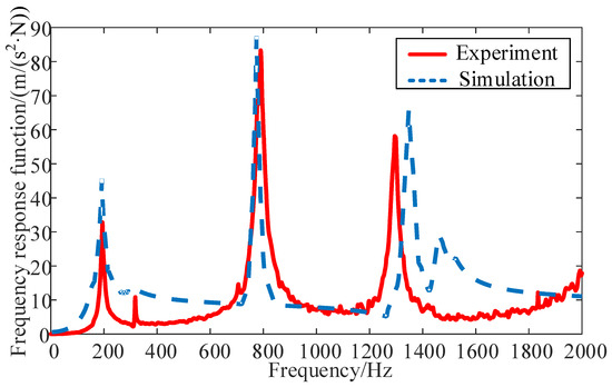
Figure 7.
Comparison of FRF between the experiment and simulation.
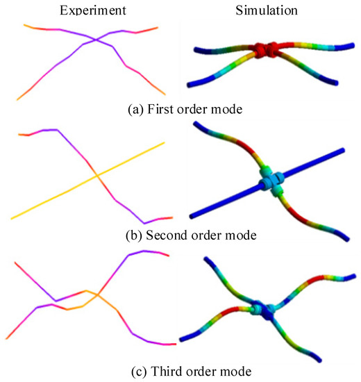
Figure 8.
Comparison of the mode shapes of the liquid-filled pipeline.
4. Influence of Different Parameters on Pipeline Vibration Characteristics
For analyzing the influence of different parameters on the dynamic characteristics, a simulation method is applied. The fluid pressures (7, 14, 21, 28, 35, 42 MPa), flow rates (0, 4, 8, 12, 16, 20 m/s), pipe diameters (6, 8, 10, 12, 14, 16, 18, 20 mm), fluids (air, kerosene, hydraulic oil, lubricating oil, water), and elastic support stiffness (103–1010 N/m), straight pipe lengths (100, 150, 200, 250, 300, 350 mm) and pipe wall thicknesses (0.5, 1, 1.5, 2, 2.5, 3 mm) are investigated by analyzing the fluid–structure interaction effect of the pipeline.
4.1. Analysis of the Flow Field in the Multi-Branch Pipeline
Figure 9 shows the flow rate, pressure and particle trajectories extracted along the central section of the pipeline. The inlet flow rate is 5 m/s, the pressure is 7 MPa, and the fluid is 46# hydraulic oil. Five lines are extracted along the pipeline section, and the schematic diagram of the extraction position is shown in Figure 10.
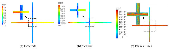
Figure 9.
Diagram of flow profile.
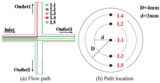
Figure 10.
Schematic diagram of the flow path.
Figure 9 shows that the fluid flow changes abruptly after passing through the joint. In the two curved parts, eddy currents are generated due to the collision between the fluid and the wall. Due to the shunting of the branch pipes, the flow rate decreases sharply after passing through the inner wall of the connection, and the flow direction of the fluid changes.
Figure 11 shows that the maximum flow rate in the pipeline before entering the joint reaches 6.84 m/s. After passing the joint, the flow rate decreases rapidly, and the minimum flow rate is 0.34 m/s Then, the pressure decreases continuously with the fluid flow path. There is an obvious low-pressure area downstream near the connection, vortices are observed in this area. The particle trajectory reveals that the fluid generates vortices due to the effects of high and low pressure. The fluid fluctuation at this location is the main cause of fluid-induced pipeline vibration.
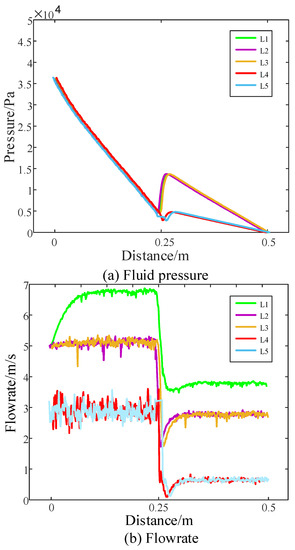
Figure 11.
The variation of the pressure and flow rate along the flow path.
4.2. The Joint Effect on Fluid-Structure Interaction
To analyze the joint effect on the fluid-structure interaction, multi-branch pipelines with and without a joint are analyzed as shown in Figure 12. The calculation iteration step is set as 0.001 s, and each step is iterated 10 times. The two-way fluid–structure interaction simulation analysis is carried out.
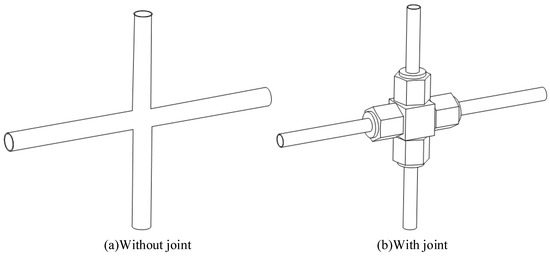
Figure 12.
Schematic diagram of pipeline with and without joint.
Figure 13 shows the deformation and equivalent stress cloud diagram of the pipeline. The difference value of the maximum deformation and equivalent stress due to the joint effect are 6.02% and 8.22%, respectively. The joint reduces the deformation of the pipeline and the value of the equivalent stress.
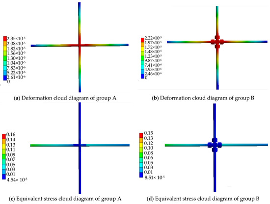
Figure 13.
Deformation and equivalent stress cloud diagram of pipelines.
Figure 14 shows the frequency response function of pipelines with and without a joint. Due to the mass effect of the joint, the natural frequencies of the pipeline shift to the low-frequency domain, and the magnitudes of FRF are significantly reduced with the addition of the joint. For engineering applications, the joint effect on the pipeline system cannot be ignored.
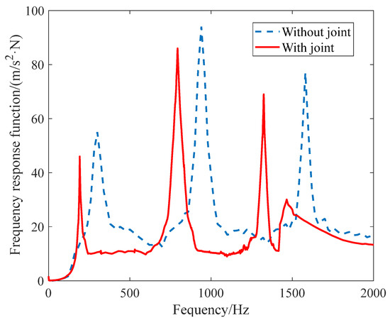
Figure 14.
Comparison of dynamic characteristic of pipelines with and without a joint.
4.3. Influence of Flow Rate on the Dynamic Characteristics of the Multi-Branch Pipeline
When the fluid pressure is set at 2 MPa, the flow rate is set at 0, 4, 8, 12, 16, and 20 m/s for analysis. Table 5 shows the first three-order natural frequencies of the pipeline at different flow rate. Figure 15 shows that the first three-order natural frequencies of the pipeline at different flow rates. The first three-order natural frequencies of the pipeline decrease continuously with the increase in flow rate, but the frequencies of each order under different flow rate are relatively close, and the change is not obvious. The first three-order natural frequencies have changed by 0.26%, 0.4%, 0.43%, respectively. The effect of the flow rate on the pipeline is due to the pressure difference caused by the variation in flow rate.
Table 5.
First three-order natural frequencies of the pipeline at different flow rate.
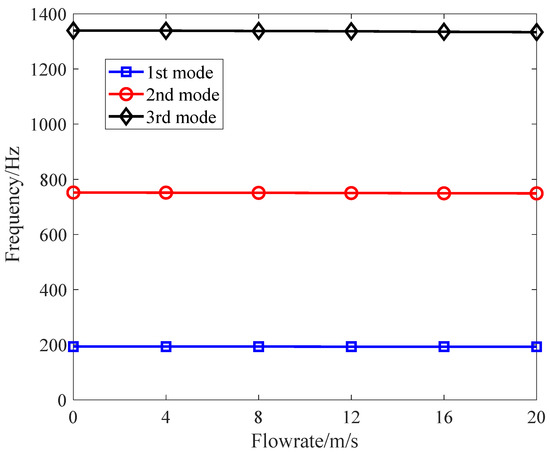
Figure 15.
First three-order natural frequencies of the pipeline at different flow rate.
4.4. Influence of Fluid Pressure on Natural Frequency of the Multi-Branch Pipeline
When the flow rate is set at 5 m/s, the fluid pressures are set at 7, 14, 21, 28, 35, and 42 MPa for analysis. Table 6 shows the first three-order natural frequencies of the pipeline at different pressures. Figure 16 shows that the first three natural frequencies of the pipeline gradually decrease with the increase in the fluid pressure. The first three-order natural frequencies are changed by 2.85%, 1.9%, and 0.62%, respectively. The influence of pressure on pipelines cannot be ignored in practical engineering analysis.
Table 6.
First three-order natural frequencies of the pipeline at different pressures.
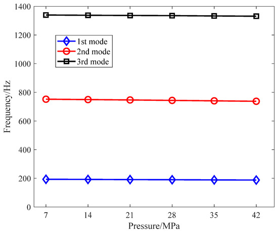
Figure 16.
First three-order natural frequencies of the pipeline at different pressures.
4.5. Influence of Fluid Medium on Natural Frequency of the Multi-Branch Pipeline
Table 7 shows the parameters of different fluids. In order to explore the effect of different fluids on the natural frequency of the pipeline, different fluids (air, aviation fuel, hydraulic oil, lubricating oil, water) are investigated.
Table 7.
Property of fluid.
Table 8 shows the first three-order natural frequencies of the pipeline with different fluids. Figure 17 shows that with the change in fluid, the first three-order natural frequencies of the pipeline gradually decrease. This change is caused by the modification of density. In different industrial fields, attention should be paid to the effect of fluid density variations on the natural frequency.
Table 8.
First three-order natural frequencies of the pipeline with different fluids.
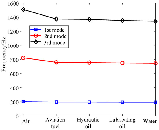
Figure 17.
First three-order natural frequencies of the pipeline with different fluids.
4.6. Influence of Pipe Diameter on Natural Frequency of the Multi-Branch Pipeline
Table 9 shows the First three-order natural frequencies of the pipeline at different pipe diameters. Figure 18 shows the first three natural frequencies of the pipeline gradually increase with the increase in pipe diameter. The first three-order natural frequencies change by 261.18%, 206.68%, and 174.58%, respectively. The size of the pipe diameter has a significant impact on the vibration characteristics of the pipeline, and the natural frequency corresponding to different pipe diameters changes obviously. The size of the pipe diameter is an important factor when it comes to the actual design. The appropriate pipe diameter size should be selected according to the actual needs to reduce costs. Avoid the resonance caused by the similar frequency of the pipeline, causing the failure of the pipeline.
Table 9.
First three-order natural frequencies of the pipeline at different pipe diameters.
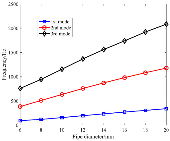
Figure 18.
First three-order natural frequencies of the pipeline at different pipe diameters.
4.7. Influence of Constraint Stiffness on Natural Frequency of the Multi-Branch Pipeline
The fixed constraint of the pipeline is changed to elastic constraint. Different restraint stiffnesses (103, 104, 105, 106, 107, 108, 109, 1010 N/m) are applied. Table 10 shows the first three natural frequencies of the pipeline at different constraint stiffness. Figure 19 shows that with the increase in restraint stiffness, the first three-order natural frequencies of the pipeline gradually increase. When the stiffness is less than 105 N/m, the pipeline is less constrained, resulting in a slow increase in the natural frequency. The elastic constraint gradually approaches the fixed constraint when the stiffness increases to 109–1010 N/m. At this point, the increase in the natural frequency becomes slow and gradually approaches the value of the natural frequency at the fixed constraint. Within this constraint stiffness range, The first three-order natural frequencies change by 2803.88%, 3374.03%, and 556.29%, respectively. When elastic restraint is applied to the pipeline, appropriate restraint stiffness shall be selected on the basis of avoiding resonance.
Table 10.
First three natural frequencies of the pipeline at different constraint stiffness.
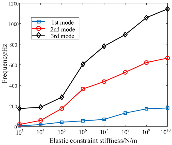
Figure 19.
First three natural frequencies of the pipeline at different constraint stiffness.
4.8. Influence of Pipe Length on Natural Frequency of the Multi-Branch Pipeline
The length of different straight pipes is set at 100, 150, 200, 250, 300, and 350 mm. Table 11 shows the first three-order natural frequencies of pipelines at different pipe lengths. Figure 20 shows that with the increase in the straight pipe length, the first three-order natural frequencies of the pipeline gradually decrease. The first three-order natural frequencies change by 793.83%, 553.61%, and 850.55%, respectively. With the increase in the pipeline length, the natural frequency path of the pipeline decreases rapidly, especially the high order mode.
Table 11.
The first three-order natural frequencies of pipelines at different pipe lengths.
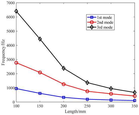
Figure 20.
The first three-order natural frequencies of pipelines at different pipe lengths.
4.9. Influence of Wall Thickness on Natural Frequency of the Multi-Branch Pipeline
The tube inner diameter is set at 10 mm. The wall thickness of the pipe is adjusted by changing the outer diameter (0.5, 1, 1.5, 2, 2.5, 3 mm). Table 12 shows the first three natural frequencies of the pipeline at different wall thicknesses. Figure 21 shows that the natural frequency of the pipeline increases with the increase in wall thickness. When the wall thickness increases, the equivalent stiffness and equivalent mass of the piping system increase. If the increasing trend of the equivalent stiffness is greater than that of the equivalent mass, this makes the natural frequency of the whole piping system increase. The first three-order natural frequencies change by 110.31%, 51.44%, and 24.35%, respectively. The selection of the pipeline should be based on the objective situation to select the appropriate wall thickness of the pipeline.
Table 12.
First three natural frequencies of the pipeline at different wall thicknesses.
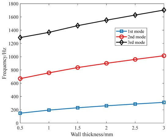
Figure 21.
First three natural frequencies of the pipeline at different wall thicknesses.
5. Conclusions
In this paper, a finite element model of a multi-branch pipeline is established and verified by experiments. The influence of different factors on the vibration characteristics of a hydraulic multi-branch pipeline is studied. The obtained conclusions are as follows:
- Fluid passing through the four-way junction changes abruptly, and the branch shunt causes a significant drop in flow rate. After the connection there is a clear low-pressure area downstream of the two branches. The particle motion trajectory indicates that the fluid generates a vortex under the influence of high and low pressure, which is the main cause of fluid-induced pipeline vibration.
- By comparing the experimental results with the finite element model, the maximum error of the first three orders of natural frequency of the pipeline is under 6.15%, which verifies the effectiveness of the model. The deformation and equivalent force of the multi-branch pipeline with a joint are reduced by more than 5%, the natural frequency and amplitude of dynamic response are smaller.
- The increasing values of flow rate and pressure reduce the natural frequency of the pipeline. The pressure has significant influence on the vibration characteristics of the pipeline. As the fluid density increases, the natural frequency of the pipeline decreases. Pipe diameter, restraint stiffness, straight pipe length, and wall thickness, etc., have large effects on the vibration characteristics of the pipeline. When the pipe diameter, elastic restraint stiffness, and wall thickness increase, the natural frequency of the pipeline increases. While the length of the straight pipe increases, the natural frequency decreases.
The multi-branch pipeline model proposed in this paper will be applied in fuel, lubricating oil, air and other pipeline systems, such as aerospace, marine, rail transit, irrigation, and petroleum etc. The above results can provide a reference for design and fabrication in the above fields.
Author Contributions
Software, Z.Z.; Validation, D.Z.; Formal analysis, Z.Z. and M.J.; Resources, T.Y. and D.Z.; Data curation, M.J.; Writing—original draft, Z.Z.; Writing—review & editing, J.J.; Supervision, T.Y. and J.J.; Project administration, T.Y.; Funding acquisition, T.Y. All authors have read and agreed to the published version of the manuscript.
Funding
This research was funded by Provincial Natural Science Foundation of China, grant number ZR2022QA041 and Provincial College youth Innovation technology project support program, grant number 2019KJB005.
Institutional Review Board Statement
Not applicable.
Informed Consent Statement
Not applicable.
Data Availability Statement
The data used to support the findings of this study are available from the corresponding author upon request.
Conflicts of Interest
The authors declare no conflict of interest.
References
- Mehmood, Z.; Hameed, A.; Javed, A.; Hussain, A. Analysis of premature failure of aircraft hydraulic pipes. Eng. Fail. Anal. 2019, 109, 104356. [Google Scholar] [CrossRef]
- Zhang, F.; Yuan, Z.; Zhang, F. The analysis and estimation of vibration fatigue for pipe fitting in aviation hydraulic system. Eng. Fail Anal. 2019, 105, 837–855. [Google Scholar] [CrossRef]
- Wang, J.; Zhang, S.Y. Field Measurement and Numerical Study of the Vibration in the Pipeline of Centrifugal Compressor. J. Press Vess-T Asme. 2019, 141, 051602. [Google Scholar]
- Tijsseling, A.A. Fluid–structure interaction in liquid-filled pipe systems: A review. J. Fluids Struct. 1996, 10, 109–146. [Google Scholar] [CrossRef]
- Wiggert, D.C.; Tijsseling, A.A. Fluid transients and fluid-structure interaction in flexible liquid-filled piping. Appl. Mech. Rev. 2001, 54, 455–481. [Google Scholar] [CrossRef]
- Zhang, L.; Tijsseling, A.S.; Vardy, A.E. FSI analysis of liquid-filled pipes. J. Sound Vib. 1999, 224, 69–99. [Google Scholar] [CrossRef]
- Ouyang, X.P.; Gao, F.; Yang, H.Y.; Wang, H.X. Two-dimensional stress analysis of the aircraft hydraulic system pipeline. Proc. Inst. Mech. Eng. Part G J. Aerosp. Eng. 2011, 226, 532–539. [Google Scholar] [CrossRef]
- Ouyang, X.; Gao, F.; Yang, H.; Wang, H. Modal Analysis of the Aircraft Hydraulic-System Pipeline. J. Aircr. 2012, 49, 1168–1174. [Google Scholar] [CrossRef]
- Andrade, D.M.; Rachid, F.B.D.F.; Tijsseling, A.S. A new model for fluid transients in piping systems taking into account the fluid–structure interaction. J. Fluids Struct. 2022, 114, 103720. [Google Scholar] [CrossRef]
- Zhang, Q.; Kong, X.; Huang, Z.; Yu, B.; Meng, G. Fluid-Structure-Interaction Analysis of an Aero Hydraulic Pipe Considering Friction Coupling. IEEE Access 2019, 7, 26665–26677. [Google Scholar] [CrossRef]
- Quan, L.; Che, S.; Guo, C.; Gao, H.; Guo, M. Axial Vibration Characteristics of Fluid-Structure Interaction of an Aircraft Hydraulic Pipe Based on Modified Friction Coupling Model. Appl. Sci. 2020, 10, 3548. [Google Scholar] [CrossRef]
- Bai, Y.; Xie, W.; Gao, X.; Xu, W. Dynamic analysis of a cantilevered pipe conveying fluid with density variation. J. Fluids Struct. 2018, 81, 638–655. [Google Scholar] [CrossRef]
- Gao, P.; Yu, T.; Zhang, Y.; Wang, J.; Zhai, J. Vibration analysis and control technologies of hydraulic pipeline system in aircraft: A review. Chin. J. Aeronaut. 2020, 34, 83–114. [Google Scholar] [CrossRef]
- Gao, P.-X.; Zhai, J.-Y.; Yan, Y.-Y.; Han, Q.-K.; Qu, F.-Z.; Chen, X.-H. A model reduction approach for the vibration analysis of hydraulic pipeline system in aircraft. Aerosp. Sci. Technol. 2016, 49, 144–153. [Google Scholar] [CrossRef]
- Gao, P.; Qu, H.; Zhang, Y.; Yu, T.; Zhai, J. Experimental and Numerical Vibration Analysis of Hydraulic Pipeline System under Multiexcitations. Shock Vib. 2020, 2020, 3598374. [Google Scholar] [CrossRef]
- Tan, X.; Ding, H.; Chen, L.-Q. Nonlinear frequencies and forced responses of pipes conveying fluid via a coupled Timoshenko model. J. Sound Vib. 2019, 455, 241–255. [Google Scholar] [CrossRef]
- Tan, X.; Ding, H. Parametric resonances of Timoshenko pipes conveying pulsating high-speed fluids. J. Sound Vib. 2020, 485, 115594. [Google Scholar] [CrossRef]
- Chai, Q.; Zeng, J.; Ma, H.; Li, K.; Han, Q. A dynamic modeling approach for nonlinear vibration analysis of the L-type pipeline system with clamps. Chin. J. Aeronaut. 2020, 33, 3253–3265. [Google Scholar] [CrossRef]
- Yuan, J.R.; Ding, H. Dynamic model of curved pipe conveying fluid based on the absolute nodal coordinate formulation. Int. J. Mech. Sci. 2022, 232, 107625. [Google Scholar] [CrossRef]
- Yuan, J.R.; Ding, H.; Chen, L.Q. Analysis and Simulation of Natural Frequencies of Slightly Curved Pipes. Appl. Math. Mech.-Engl. Ed. 2022, 43, 719–726. [Google Scholar]
- Wiggert, D.C.; Hatfield, F.J.; Stuckenbruck, S. Analysis of Liquid and Structural Transients in Piping by the Method of Characteristics. J. Fluids Eng.-T Asme 1987, 109, 161–165. [Google Scholar] [CrossRef]
- Lesmez, M.W.; Wiggert, D.C.; Hatfield, F.J. Modal Analysis of Vibrations in Liquid-Filled Piping Systems. J. Fluids Eng.-T Asme 1990, 112, 311–318. [Google Scholar] [CrossRef]
- Wylie, E.B.; Streeter, V.L.; Wiggert, D.C. Fluid transients. J. Fluid Eng.-T Asme 1980, 102, 384. [Google Scholar] [CrossRef]
- Dai, H.; Wang, L.; Qian, Q.; Gan, J. Vibration analysis of three-dimensional pipes conveying fluid with consideration of steady combined force by transfer matrix method. Appl. Math. Comput. 2012, 219, 2453–2464. [Google Scholar] [CrossRef]
- Kalliontzis, D. Fluid–structure interaction with ALE formulation and skeleton-based structural models. J. Fluids Struct. 2022, 110, 103513. [Google Scholar] [CrossRef]
- Huang, Y.M.; Liu, Y.S. Natural frequency analysis of fluid conveying pipeline with different boundary conditions. Nucl. Eng. Des. 2010, 240, 461–467. [Google Scholar]
- Zhu, H.J.; Zhang, W.; Feng, G. Fluid–structure interaction computational analysis of flow field, shear stress distribution and deformation of three-limb pipe. Eng. Fail Anal. 2014, 42, 252–262. [Google Scholar] [CrossRef]
- Franci, A. Lagrangian finite element method with nodal integration for fluid–solid interaction. Comput. Part. Mech. 2020, 8, 389–405. [Google Scholar] [CrossRef]
- Lavooij, C.S.; Tijsseling, A.S. Fluid-structure interaction in liquid-filled piping systems. J. Fluid Struct. 1991, 5, 573–595. [Google Scholar] [CrossRef]
- Wang, Z.; Tan, S. Vibration and pressure fluctuation in a flexible hydraulic power system on an aircraft. Comput. Fluids 1998, 27, 1–9. [Google Scholar] [CrossRef]
- Liu, G.; Li, S.; Li, Y.; Chen, H. Vibration analysis of pipelines with arbitrary branches by absorbing transfer matrix method. J. Sound. Vib. 2013, 332, 6519–6536. [Google Scholar] [CrossRef]
- Neto, H.R.; Cavalini, J.A.; Vedovoto, J.M.; Neto, A.S.; Rade, D.A. Influence of seabed proximity on the vibration responses of a pipeline accounting for fluid-structure interaction. Mech. Syst. Signal Pr. 2019, 114, 224–238. [Google Scholar] [CrossRef]
- Wu, G.X.; Zhao, X.L.; Shi, D.D.; Wu, X.D. Analysis of fluid–structure coupling vibration mechanism for subsea tree pipeline combined with fluent and Ansys workbench. Water 2021, 13, 955. [Google Scholar] [CrossRef]
- Wu, J.; Li, C.; Zheng, S.Y.; Gao, J.H. Study on fluid-structure coupling vibration of compressor pipeline. Shock Vib. 2019, 12, 8624324. [Google Scholar] [CrossRef]


Publisher’s Note: MDPI stays neutral with regard to jurisdictional claims in published maps and institutional affiliations. |
© 2022 by the authors. Licensee MDPI, Basel, Switzerland. This article is an open access article distributed under the terms and conditions of the Creative Commons Attribution (CC BY) license (https://creativecommons.org/licenses/by/4.0/).