Abstract
The working environment of tractors is harsh and the working conditions are very complicated. To cope with this complex and changeable working environment, this paper presents a hybrid tractor powertrain loaded with hydraulic mechanical combined transmission (HMCVT). The powertrain can switch modes according to different operating environments. During mode switching, impact loads can cause wear and even damage to the transmission components. Interrupting the power transmission will reduce the tractor’s operational efficiency. In this paper, the orthogonal experimental range analysis method was proposed to optimize the quality of mode switching. Mode switching involves interactions between clutches. Orthogonal table L16 (215) was selected to design the orthogonal table head. SimulationX was used for simulation. Employing MINITAB range analysis yielded the optimal results. The simulations indicated a reduction in the output shaft’s velocity drop amplitude from 17.647% to 6.591%. The dynamic load coefficient decreased from 2.743 to 1.857. The impact strength was reduced from 14.125 to 5.67 m/s3. The switching time was reduced from 2.13 to 1.71 s. We built a model-in-the-loop (MIL) test platform to validate the results. The MIL test results were compared with the simulation results. Our findings indicate a degree of discrepancy between the simulated and the experimental results, yet the overall trends remain largely consistent. The correctness of the optimal scheme obtained from the orthogonal experiment is verified. This study provides a theoretical basis for the optimization of powertrain mode switching in hybrid tractors equipped with HMCVT.
1. Introduction
As the core piece of equipment involved in agricultural mechanization, the tractor has completely changed the traditional mode of agricultural production with its power and versatility. It has replaced human and animal power, significantly improved farming’s efficiency, and undertakes important tasks such as farmland cultivation, sowing, field management and transportation by pulling and driving various working machinery, providing support to the large-scale and intensive development of agricultural production [1].
In recent years, with the modernization of China’s agriculture, tractor technology and equipment are constantly being updated and improved [2]. The research and development and application of advanced high-horsepower tractors and supporting agricultural machinery have provided a strong technical basis for moderate scale operations and full mechanized production, especially in areas with complex terrain such as hills and mountains, playing an irreplaceable role. At the same time, national policies also actively guide the agricultural machinery industry to develop in the direction of intelligence and information technology and promote the development of high quality, high efficiency, and ecologically friendly agricultural production [3].
Hybrid tractors loaded with an HMCVT have a variety of operating modes. The HMCVT can provide power and reduce fuel consumption. However, to take full advantage of these advantages, smooth and precise mode switching is essential. During mode switching, impact loads can cause wear or even damage to the transmission components. Frequent vibration will affect the operator’s comfort. The interruption of power transmission will reduce the efficiency of operation. These problems can have a negative impact on the ride and operating fluency of the tractor and shorten the service life of the transmission system [4].
Chen has proposed an optimization strategy based on shift parameter matching. Through simulation analysis, the influence of optimized front and rear shifting parameters on the sliding friction during the operation of the clutch is compared. The results show that the optimized shift parameters can effectively reduce the sliding friction during the operation of the clutch under nine farming conditions, and significantly improve the efficiency of the tractor’s transmission system and the smoothness of the shift [5]. YU proposes a control strategy based on Variable Universe Fuzzy PID. The simulation results show that the variable domain fuzzy PID controller reduces the HMCVT speed by about 50% compared with the tracking error [6]. Li introduces a dual-circuit control method for pump-motor hydraulic systems. This strategy not only ensures that there is no interference in the control signal during fixed displacement but also enhances response characteristics and output stability during displacement ratio adjustments. The simulation results indicate that the implemented control strategy can achieve a 64.4% reduction in shift acceleration [7]. Zhao presents an adaptive control approach employing radial basis function neural networks and proportional–integral–derivative control. The simulation and experimental outcomes demonstrate a rapid target speed response during launch with minimal fluctuation across varying initial input speeds [8]. Lu introduced a global terminal sliding mode control algorithm based on an extended observer, which achieves high-precision pressure tracking control. This control strategy reduces the maximum jump vibration by 12.7% and the maximum sliding friction during operation by 10.2% [9].
The existing research mainly focuses on optimizing the fluctuations caused by internal shocks in the HMCVT, while ignoring the fluctuations caused by the engagement and disengagement of external clutches during mode switching, especially the mutual influence between clutches. This article aims to study an optimization method for the switching process between hydraulic mode and mechanical hydraulic compound transmission mode, to improve the smoothness and efficiency of mode switching, reduce impact loads and vibrations, and avoid power transmission interruptions.
This article proposes a new optimization method that considers the interactions between clutches during mode switching. Suitable orthogonal meter heads were designed through orthogonal experimental methods. The optimal clutch switching timing can be obtained, effectively improving the quality of clutch mode switching and reducing the fluctuation of the transmission system. Finally, the effectiveness of this method was verified through MIL testing. The research results can provide a theoretical reference for the development of control strategies for the process of switching from hydraulic mode to mechanical hydraulic compound transmission mode.
The rest of this article is structured as follows. In the Section 2 we analyze the transmission process in hydraulic mode and mechanical hydraulic mode and establish a transmission system model using SimulationX 3.5 software. The Section 3 establishes evaluation indicators for mode switching. To enhance the smoothness of mode switching from hydraulic to mechanical-hydraulic operation, an optimization approach based on orthogonal experimental range analysis is proposed. In the Section 4 we establish hardware for the loop experimental platform, use the orthogonal experimental variance method for result analysis, and compare the analysis results with simulation results. Section 5 is a summary of the entire text.
2. Transmission Mode Analysis and System Modeling
2.1. Transmission Mode Analysis
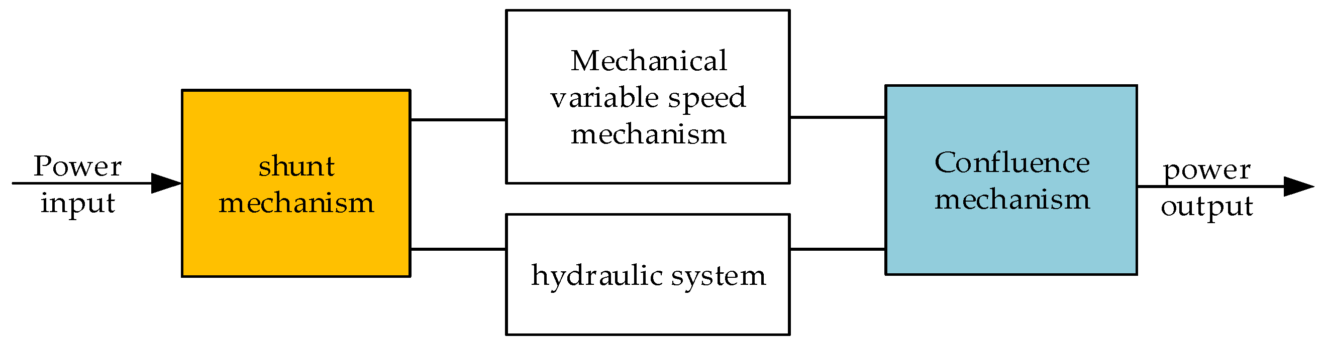
Figure 1 shows the basic transmission principle of mechanical hydraulic composite transmission [10]. The power input to the shunt mechanism divides the total power flow into two parts: one part flows through the hydraulic system, and the other flows through the mechanical variable speed mechanism, and the two power flows are coupled into the total power flow output in the confluence mechanism. A mechanical hydraulic composite transmission device not only has the advantage of stepless speed regulation of the hydraulic transmission, but also has the high efficiency and stability of mechanical transmission [11].
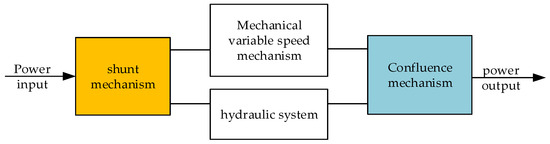
Figure 1.
The principle of mechanical hydraulic composite transmission.
The directions of the speed and torque in the shunting mechanism and the confluence mechanism are shown in Figure 2. The shunting mechanism (a) and the confluence mechanism (b) adopt a planetary gear mechanism, which includes the sun wheel, gear ring, and planetary frame. The speed relationship between the three is constrained by the characteristic formula shown in Equation (1), and the torque relationship between the three has a fixed proportion, while the speed relationship among the three does not have a fixed proportion. As shown in Equation (2):
where , , and , respectively, represent the rotational speeds of the sun gear, ring gear, and planetary carrier in the planetary gear; TS, TR, and TC, respectively, represent the torque of the sun gear, ring gear, and planetary carrier; k is the characteristic parameter of the planetary arrangement.
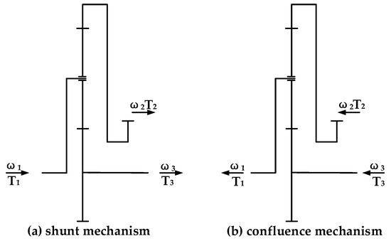
Figure 2.
Transmission principle of shunt mechanism and confluence mechanism.
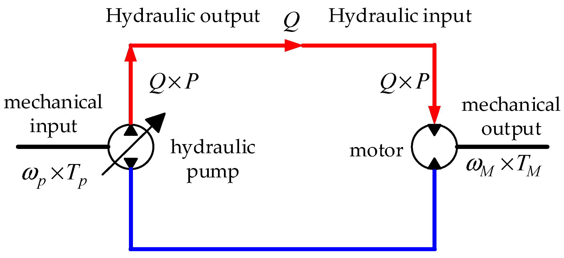
The core of implementing a continuously variable speed in HMCVT lies in the hydraulic system. Hydraulic systems typically use a volumetric speed control circuit composed of variable displacement pumps and quantitative motors to achieve high-power transmission. By changing the working volume of the pump, the displacement of the hydraulic pump can be adjusted to achieve stepless speed regulation. As shown in Figure 3, the prime mover serves as the power source to drive the hydraulic pump, converting mechanical energy into pressure energy in the oil. The hydraulic system circuit transfers pressure energy to the motor in the form of flow and pressure. The motor converts the pressure energy from the oil into mechanical outputs in the form of torque and speed, driving the actuator to complete its work.
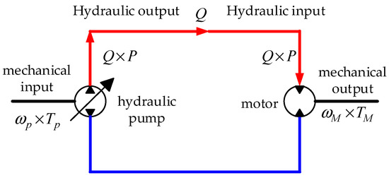
Figure 3.
Pump-motor drive system.
In the actual operation of hydraulic systems, power loss is inevitable, mainly including volume loss caused by oil leakage and mechanical losses caused by friction during the operation of mechanical components. In an ideal scenario, without considering volumetric and mechanical losses, according to the law of conservation of energy, the input–output relationship between the pump and motor can be expressed as:
where TP and TM represent the input torque of the pump and the output torque of the motor, respectively; and represent the input shaft angular velocity of the pump and the output shaft angular velocity of the motor, respectively; and represent the pressure difference between the inlet and outlet ports of the pump and motor, respectively; and , respectively, represent the output flow rate of the pump and the input flow rate of the motor.
The values of the transmission system characteristic parameters of HMCVT are shown in Table 1.

Table 1.
HMCVT transmission parameter assignment.
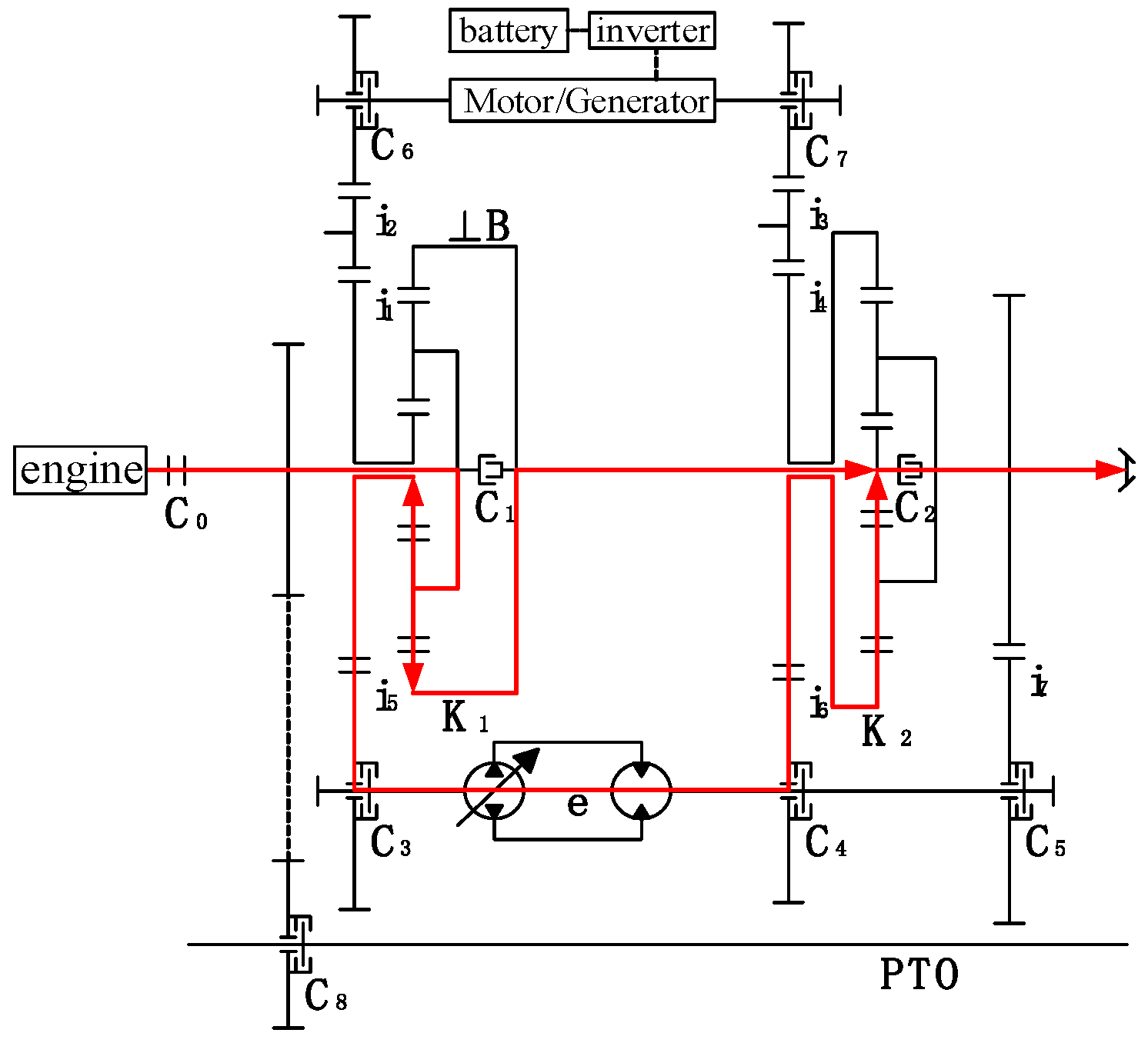
The hydraulic mode is driven by the engine, which is suitable for the starting condition of the tractor at a low speed and a large torque, and the hydraulic system can carry out efficient stepless speed regulation when the tractor is working [12]. The vehicle enters hydraulic mode after engaging the clutches C0, C1, C3, and C5. The engagement of clutch C1 immobilizes the front planetary gear mechanism, creating a unified structure. The power provided by the engine passes through the front planetary gear mechanism and enters the hydraulic system. After the power flows out of the hydraulic system, it is finally output from the output shaft. The transmission route of the hydraulic mode is shown in Figure 4. The speed relationship between its input and output is shown in Equation (4)
where no represents output shaft speed; e represents the pump-motor displacement ratio; ne represents engine output speed; i represents the gear pair ratio.
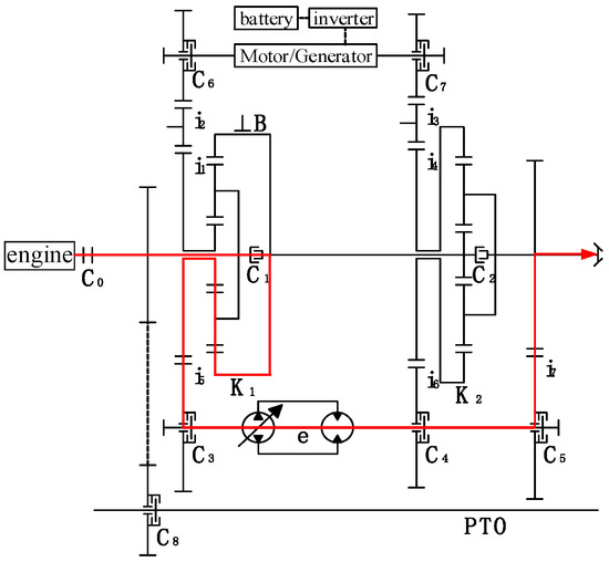
Figure 4.
Hydraulic mode transmission route.
The mechanical hydraulic compound transmission mode is driven by the engine. The shunt mechanism can expand the speed regulation range of the hydraulic mechanism. And it can realize the linear stepless speed regulation of the vehicle, which can reduce the operating difficulty of the driver and improve the working quality. Moreover, it can meet the higher power requirements of tractors, and further improve the power performance and fuel efficiency of the whole vehicle [13].
After engaging the clutches C0, C2, C3, and C4, the tractor enters the mechanical hydraulic compound transmission mode. The transmission route of the mechanical hydraulic compound transmission mode is shown in Figure 5. The power provided by the engine is divided between two paths after entering the front planetary array. One path goes into the front planetary sun wheel and flows into the hydraulic system. The other path goes into the front planetary gear ring and flows to the sun wheel of the back planetary row. The two power flows eventually converge and are output from the rear planetary row. The speed relationship between the input and the output is shown in Equation (5):
where k1 represents the characteristic parameter of the front planetary row.

Figure 5.
The mechanical hydraulic compound transmission mode.
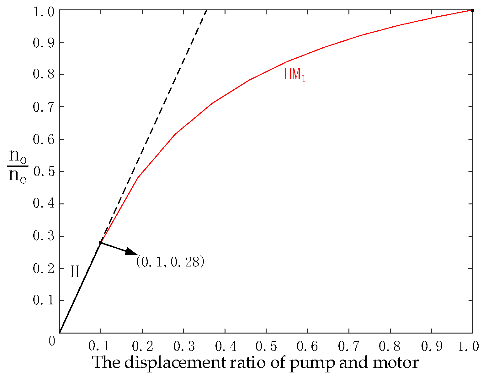
The speed regulation characteristic curve of the transmission process from hydraulic mode to A mode is shown in Figure 6. In the figure, no represents the output shaft speed, H represents the hydraulic mode speed regulation characteristic curve, HM1 represents the mechanical hydraulic composite transmission mode speed regulation characteristic curve, and (0.1, 0.28) represents the hydraulic system displacement ratio and output input speed ratio corresponding to the switching from hydraulic mode to mechanical hydraulic composite transmission mode.
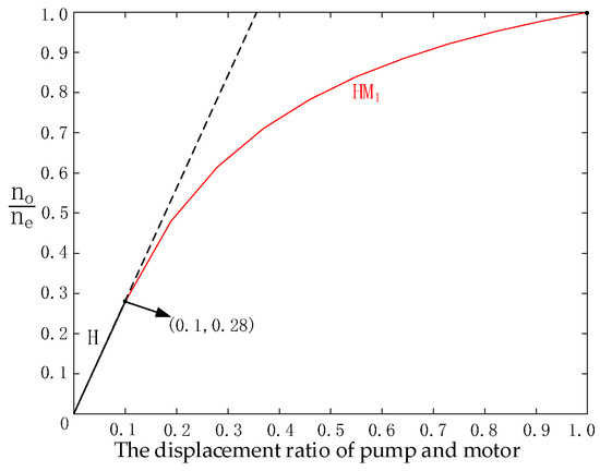
Figure 6.
Speed regulation characteristic curve.
2.2. Simulation Model Theoretical Modeling
One way to build an engine model is to perform a theoretical analysis of the engine at different times and use mathematical models to model and analyze it, but the engine is a complex nonlinear system, so the difficulty of the modeling and calculation is significant [14]. Another approach leverages bench test data to construct an interpolation model, providing a relatively simple and intuitive method for implementation [15].
An interpolation modeling method, grounded in bench test data, is employed to facilitate the development of an accurate engine model in this research. A series of dynamometer bench tests were performed on a Weichai WP6.180E40 engine, with the primary objective of recording engine output speed, torque, and throttle opening data. A 3D map correlating engine speed, torque, and throttle opening was then generated using data interpolation, as depicted in Figure 7.
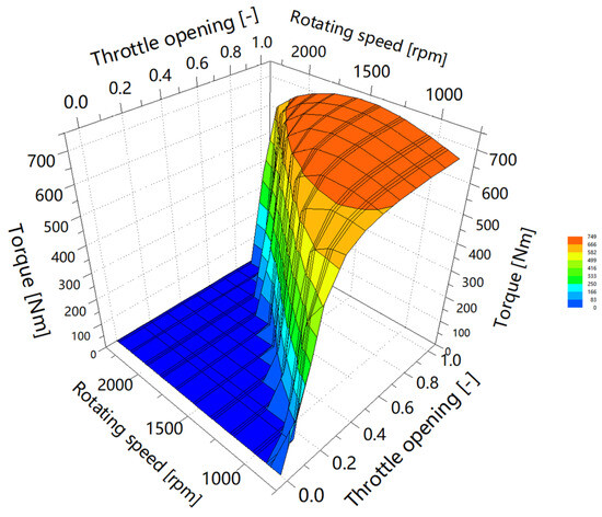
Figure 7.
Engine theoretical model.
Engine output torque can be numerically modeled as:
where α represents throttle opening; Te represents engine torque; ne represents engine speed.
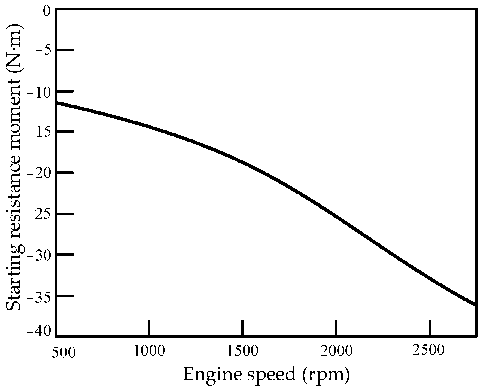
The starting resistance moment is added to simulate the cold starting process of the engine, as shown in Figure 8. With the increase in the starting speed, the average backward towing torque generated also increases, and the reverse towing torque eventually presents an approximate linear relationship with the increase in engine speed [16].
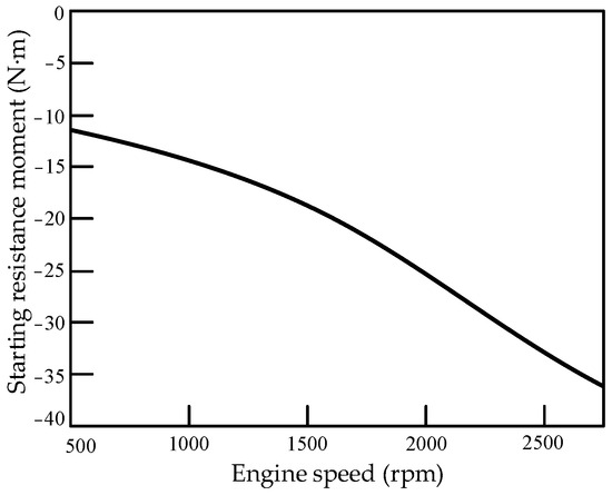
Figure 8.
Engine starting resistance moment model.
The hydraulic system consists of a variable pump and a quantitative motor. This article sets the closed circuit of the hydraulic system in an ideal state, ignoring the circuit volume and mechanical losses. The pump and motor are set to have no friction loss and leakage during operation. Therefore, the output flow rate QP of the pump is equal to the input flow rate QM of the motor.
The quantitative motor displacement is shown in Formula (8):
where DM is the quantitative motor displacement; TM is the output torque of the quantitative motor; Δp is the quantitative motor working pressure; ηM is the quantitative motor mechanical efficiency.
The quantitative motor flow rate is presented in Equation (9):
where nm is the output speed of the quantitative motor; ηv1 is the volumetric efficiency of the motor.
Variable pump displacement is Formula (9):
where DP is variable pump displacement; np is variable pump input speed; ηv2 is the variable pump volumetric efficiency.
2.3. Simulation Model Establishment
ITI is one of the leading software and engineering companies in the field of system simulation. ITI’s SimulationX is a standard tool for evaluating component interactions within technical systems. It fully supports the Modelica language and allows users to incorporate the required equations into the model according to their needs, so secondary development is easy [17].
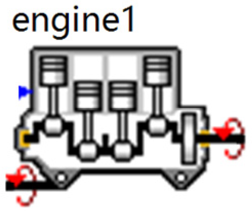
The Power Transmission library of SimulationX software has its own engine model, as shown in Figure 9. This model is an engine crankshaft angle control model based on theory. Users are unable to modify the internal characteristics of the engine. Therefore, the model is not suitable for the engine model based on the data measured from the bench.

Figure 9.
Combustion engine model.
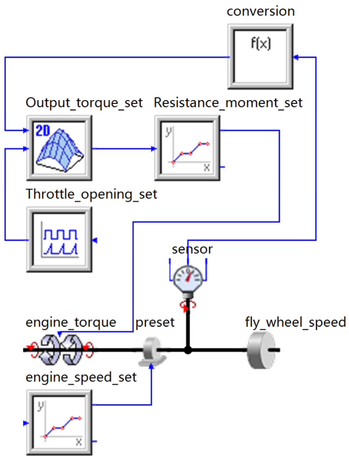
According to the modeling method used for the experimental data, an engine model suitable for the measured model was established in this paper, as is shown in Figure 10.
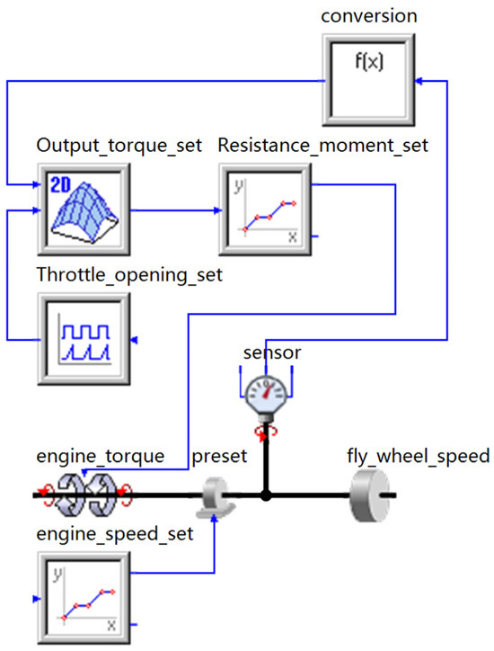
Figure 10.
Engine simulation model.
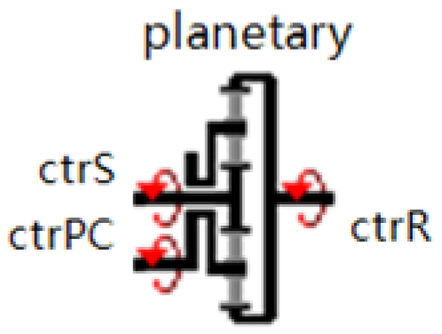
The shunt mechanism is composed of a planetary gear model. We used the Planetary Gearbox model from the Transmission Elements library in the SimulationX software, as shown in Figure 11. Among them, “ctrS” denotes the planetary gear mechanism’s sun gear, “ctrPC” represents its planetary carrier, and “ctrR” signifies its ring gear.

Figure 11.
Planetary gear model.
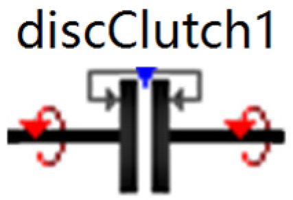
The clutch model in this paper is a wet clutch. The Disc Clutch model in the Power Transmission library in SimulationX software was adopted, as shown in Figure 12.

Figure 12.
Disc Clutch model.
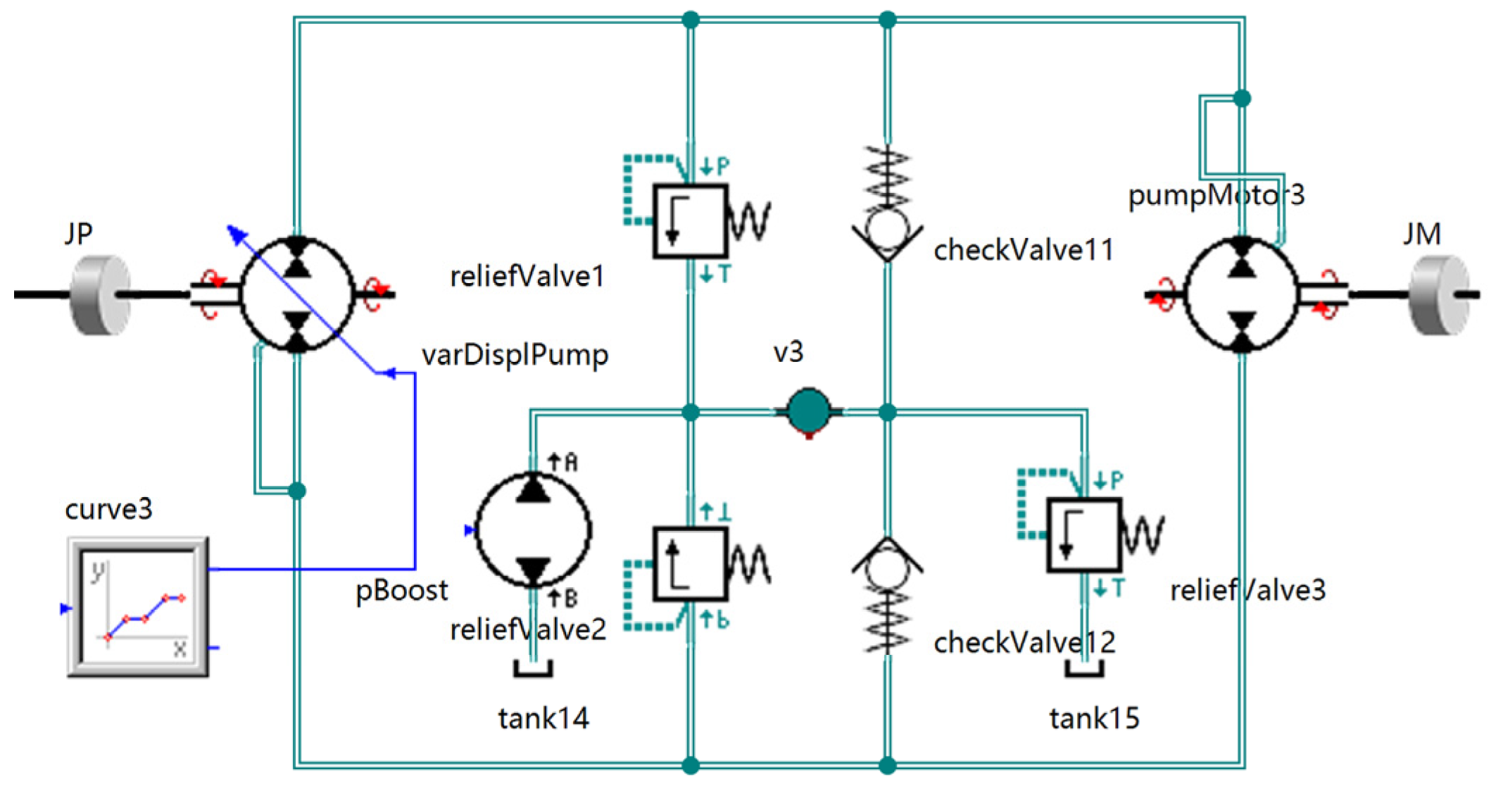
We adopted a variable pump-quantitative motor system to achieve stepless speed regulation. Its design was simple and it had only a small temperature rise. This study used a smaller load torque of 100 N∙m, a smaller main oil pressure of 3.5 MPa, and a larger speed control valve flow rate of 5 L/min. The purpose of this was to reduce the impact of hydraulic systems on the results. The hydraulic speed control module is shown in Figure 13.
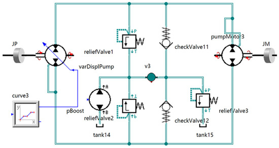
Figure 13.
Hydraulic speed control module.
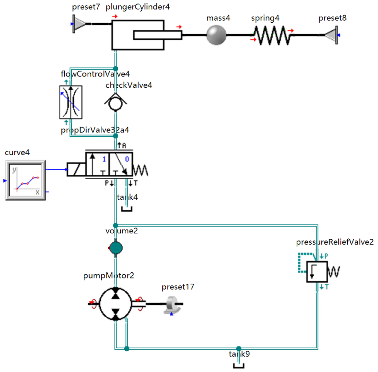
The clutch hydraulic control system module consists of a hydraulic system, as shown in Figure 14. This can be used to control the timing of the engagement and separation of Disc Clutch models. The clutch can essentially be reduced to an oil cylinder with a specified mass, and the piston inside the cylinder moves under the combined action of the oil pressure and the return spring. The oil pressure valve of the main oil circuit controls the oil filling pressure, the relief valve of each branch regulates the oil filling flow to ensure the oil filling time, and the check valve is responsible for rapid oil discharge by controlling the solenoid valve on and off to control the clutch connection and separation operation.
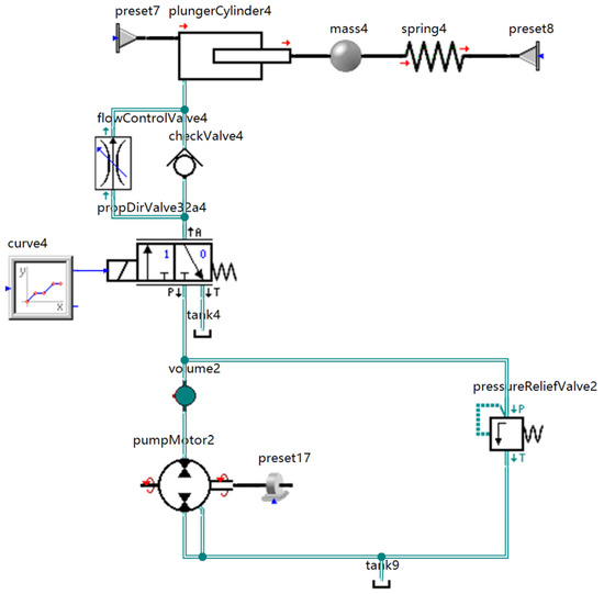
Figure 14.
Clutch hydraulic control module simulation model.
3. Optimization of Switching Process from Hydraulic Mode to Mechanical Hydraulic Compound Transmission Mode
3.1. Evaluation of Indicators of Mode Switching Quality
Output shaft speed fluctuation during mode switching is quantified by the velocity drop amplitude. There are many reasons for the increase or decrease in output shaft speed, such as energy loss caused by various frictional forces in mechanical transmission, sudden changes in load leading to speed changes, and vibrations and impacts caused by system mode switching. The velocity drop amplitude of the output shaft is a key indicator of mode switching quality. The expression is:
where is the steady output speed of the output shaft, is the lowest output speed of the output shaft, and is the speed drop amplitude of the output shaft.
During the mode switching process, the engagement and disengagement of the clutch will cause the internal oil pressure to fluctuate dramatically. The fluctuations in the oil pressure will directly affect the transmission torque of the clutch, and then cause the torque of the output shaft to change, affecting the ride comfort and driving experience of the vehicle. To quantify the fluctuation degree of output shaft torque, the concept of dynamic load coefficient of output shaft is introduced [18]. Its expression is:
where is the maximum torque of the output shaft, is the steady-state output torque of the output shaft, and is the dynamic load coefficient of the output shaft.
The output shaft impact strength describes the change rate of acceleration of the vehicle. A smaller value indicates that the vehicle is more stable during mode switching. The Chinese standard for impact strength is |J| ≤ 17.64 m/s3. Its expression is:
where rq is the radius of the driving wheel; ir is the rear axle transmission ratio; and J is the impact strength of the output shaft.
The mode switching time is an important index that can be used to measure the efficiency of mode switching, which is defined as the time required for the output shaft speed to transition from a stable state in one mode to a stable state in another mode. To accurately measure the switching time, this paper defines mode switching completion as the point at which output shaft speed reaches 99% of the target mode’s stable speed.
3.2. Orthogonal Experiment Design
Orthogonal tests transform engineering problems into mathematical problems and simplify the calculation of statistical analysis through the two steps of “test design” and “data processing”, thus saving a lot of test time and economic costs. Orthogonal testing encompasses range analysis and variance analysis methods. The range analysis method is suitable for a situation where the simulation results are relatively accurate and can intuitively judge the influence degree of each factor on the evaluation index. The analysis of variance is applicable to situations with large test errors and can quantify the importance of various factors to the test results [19].
The switching process from hydraulic mode to hydraulic mechanical compound transmission mode involves the switching of four clutches, namely clutches C1, C2, C4, and C5. The four clutches are considered as factors in the range analysis of the orthogonal test and are set as A, B, C, and D. The output shaft speed reduction amplitude, output shaft dynamic load coefficient, impact strength, and switching time are set as evaluation indicators I, II, III, and IV, respectively. Then, 20 s is taken as the on-time switching point of the simulation, and the two levels are set as 19.5 s for the switching clutch and 20 s for the just-in-time switching clutch. We then considered the pairwise interaction between the four factors. According to the orthogonal table commonly used in orthogonal experiments, the L16(215) orthogonal table was used to carry out the experiment, and a total of 16 simulations needed to be completed. The orthogonal table generated by the MINITAB 17 software is shown in Table 2.
Table 2.
L16(215) orthogonal table.
3.3. Analysis of Simulation Results Obtained Using the Range Method
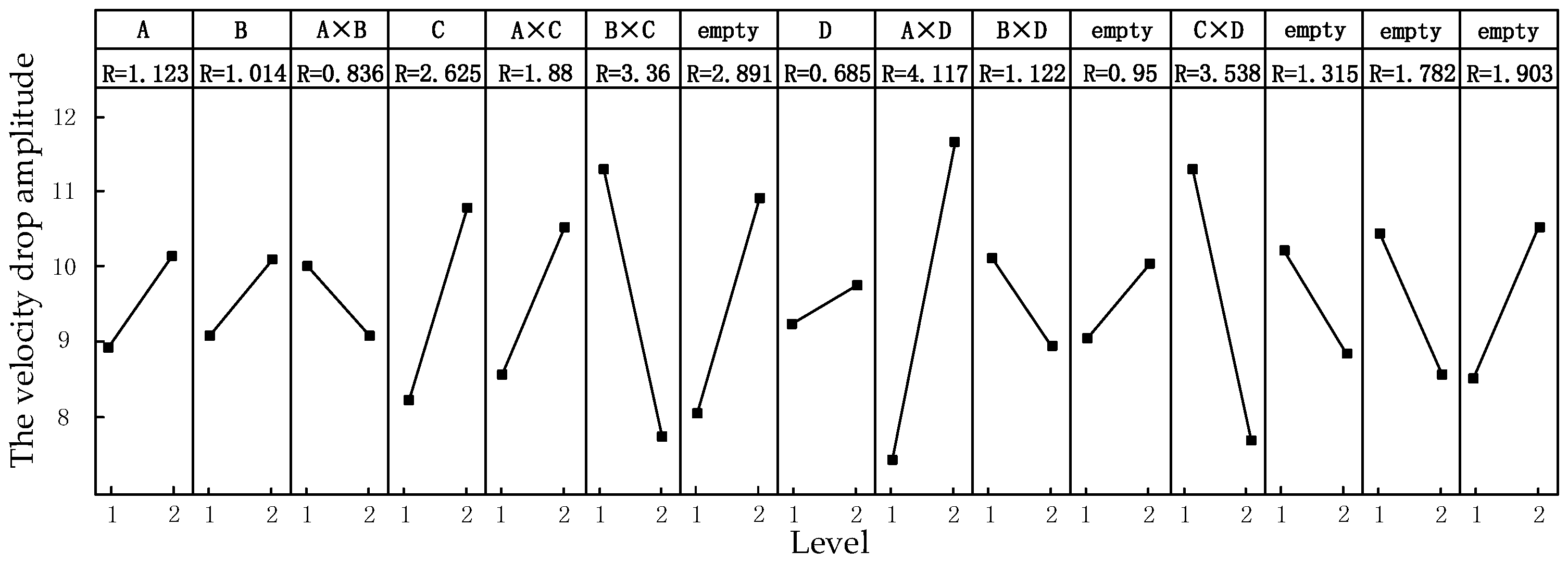
An analysis of the results for the velocity drop amplitude obtained using the range analysis method can be seen in Figure 15, which presents the range analysis results for the output shaft, with R representing the range value. According to the range value R, from large to small, the primary and secondary order of each factor and interaction is A × D, C × D, B × C, C, A × C, A, B × D, B, A × B, D.
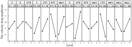
Figure 15.
Analysis results of velocity drop amplitude.
First, the collocation effect of A × D, C × D and B × C was considered to determine the optimal treatment combination. The collocation effect of A × D is calculated as shown in Table 3(a), and it was concluded that A1D1 is the optimal horizontal combination of A and D.
Table 3.
The collocation effect of velocity drop amplitude.
The collocation effect of C × D is calculated as shown in Table 3(b). It was concluded that D2C1 is the optimal level combination of C and D, but to maintain consistency with the optimal level D1 determined by the former equation, D1C2 is finally determined as the optimal level combination of C and D.
Similarly, by calculating the collocation effect of B × C, as shown in Table 3(c), C2B1 was found to be the optimal horizontal combination of B and C.
In summary, the optimal scheme to optimize the output shaft velocity drop is A1D1C2B1, which can reduce the output shaft speed drop from 17.647% to 6.233%.
Figure 16 presents the range analysis results for the output shaft’s dynamic load coefficient. According to the range value R, from large to small, the primary and secondary order of each factor and interaction is A × D, C × D, B × C, C, A × C, B, B × D, A × B, D, A.
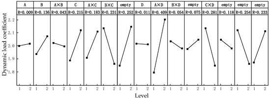
Figure 16.
Analysis result of dynamic load coefficient of output shaft.
Similarly, based on the collocation effects shown in Table 4(a–c), the optimal scheme for minimizing the output shaft’s dynamic load coefficient is A2D2C1B2, reducing it from 2.743 to 1.544.
Table 4.
The collocation effect of dynamic load coefficient.
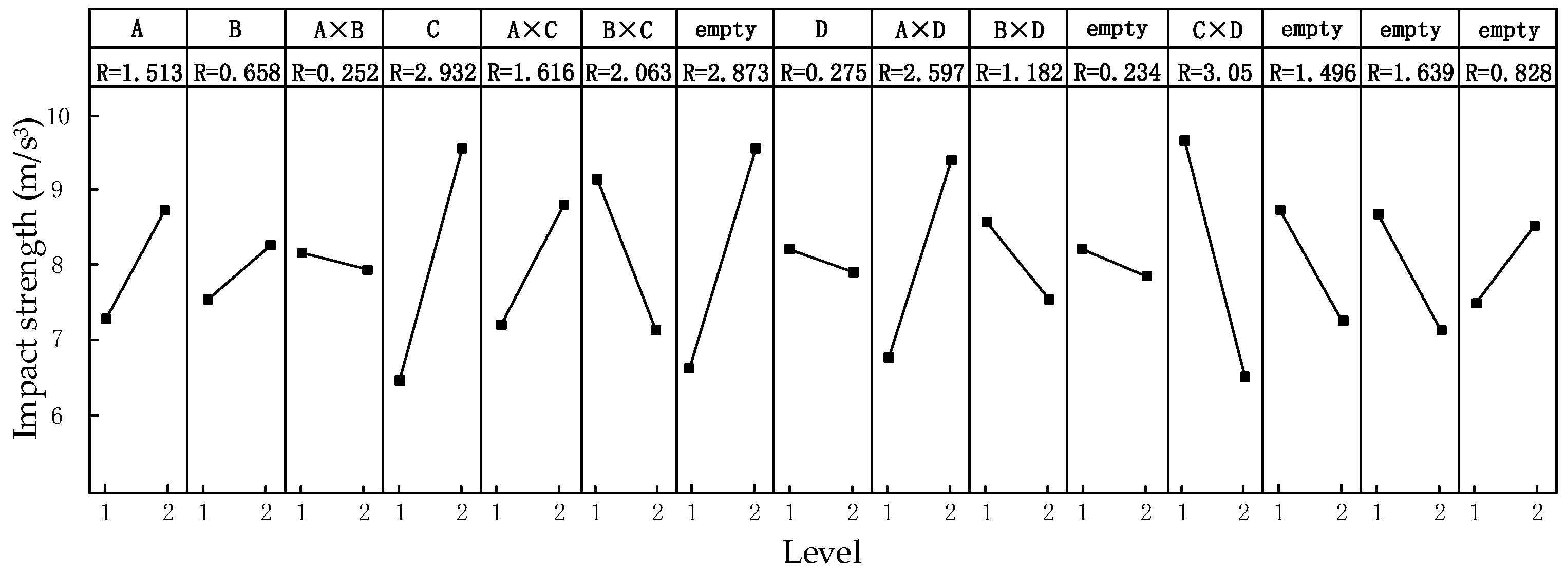
Figure 17 displays the range analysis results for the output shaft’s impact strength. According to the range value R, the major to minor order of each factor and interaction is C × D, C, A × D, B × C, A × C, A, B × D, B, D, A × B.
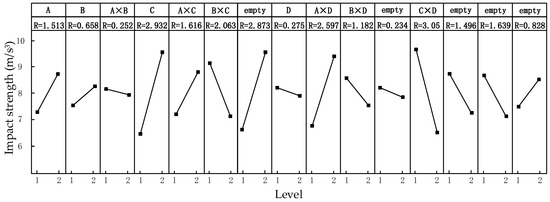
Figure 17.
Analysis result of impact strength of output shaft.
Based on the collocation effects in Table 5(a–c), the optimal scheme to optimize the impact strength of the output shaft is C1D2A2B2, which can reduce the impact of the output shaft from 14.125 to 2.23 m/s3.
Table 5.
The collocation effect of impact strength.
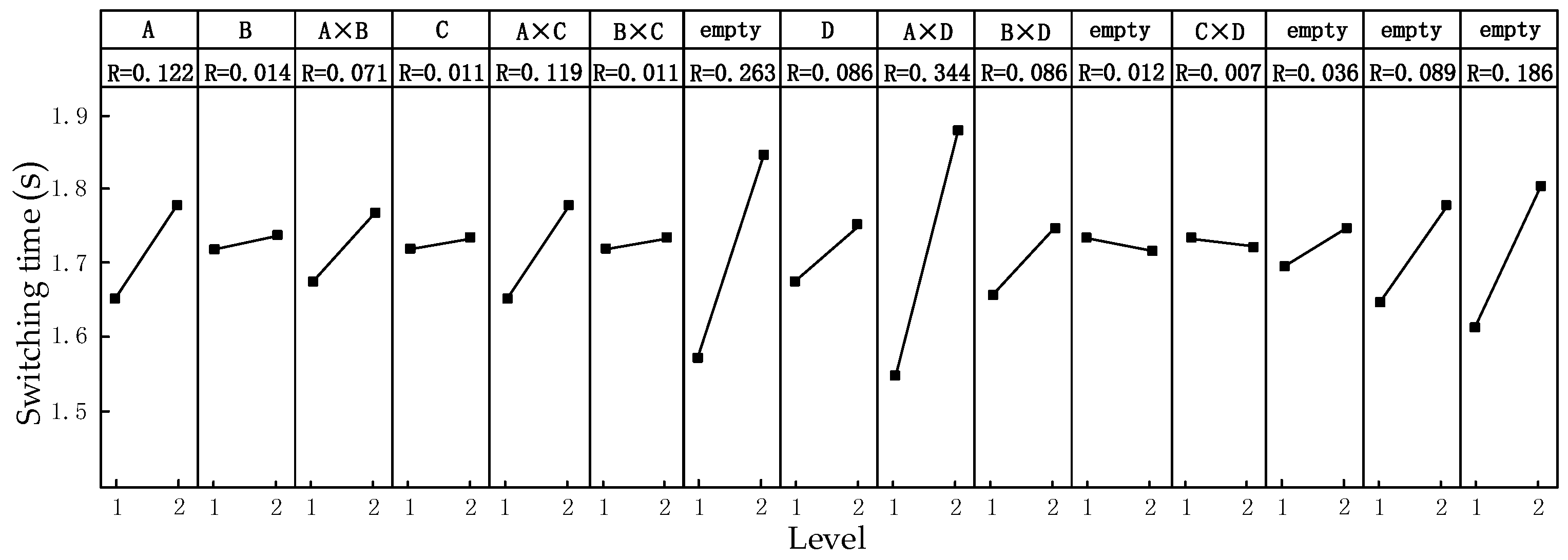
Figure 18 displays the range analysis results for switching time. According to the range value R, from large to small, the primary and secondary order of each factor and interaction is A × D, A, A × C, B × D, D, A × B, B × C, C × D.
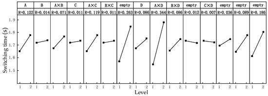
Figure 18.
Analysis result of switching time.
Based on the collocation effects in Table 6(a–c), the optimal scheme to optimize the switching time is A1D1C1B1, which can reduce the switching time from 2.13 to 1.01 s.
Table 6.
The collocation effect of switching time.
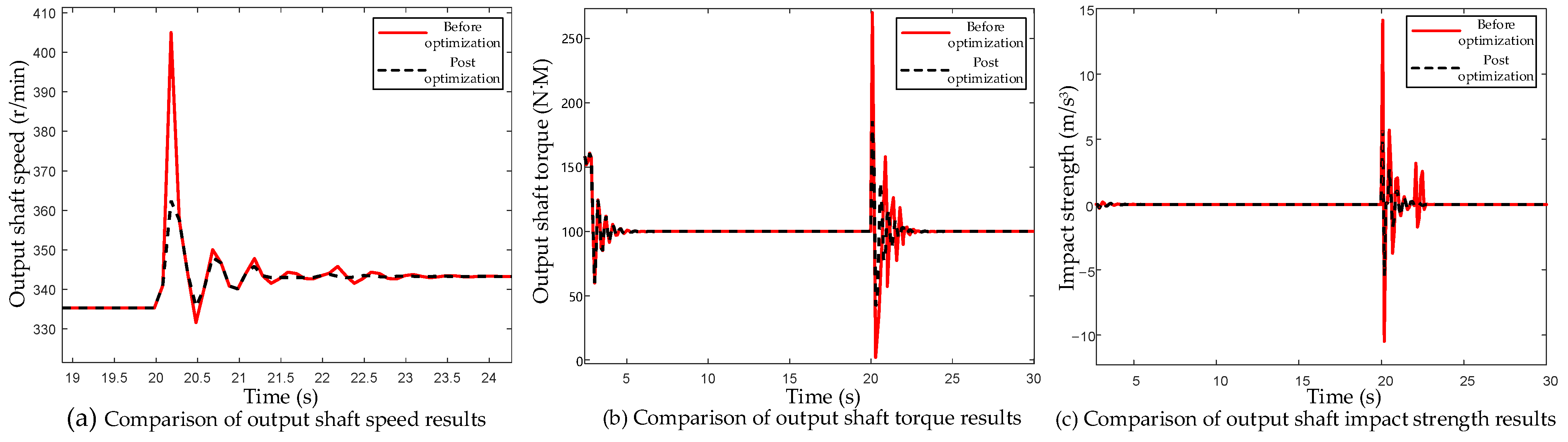
According to the above evaluation indexes, A1D1C1B2 is the overall optimal scheme. The simulation results of the overall optimal scheme and the non-optimized scheme are compared. Figure 19a shows the velocity of the output shaft. Using Equation (10), the reduction in the output shaft speed was found to decrease from 17.647% to 6.591%. Figure 19b illustrates the output shaft torque. Applying Equation (11), the output shaft dynamic load coefficient was found to decrease from 2.743 to 1.857. Figure 19c demonstrates a reduction in the output shaft impact strength from 14.125 to 5.67 m/s3, accompanied by a decrease in switching time from 2.13 to 1.71 s.
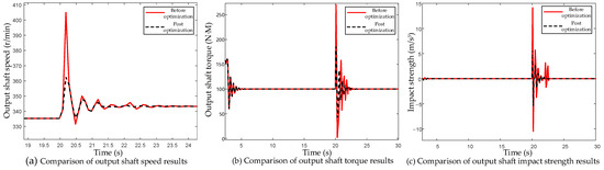
Figure 19.
Simulation data before and after optimization.
A comparison of the results before and after optimization, as well as the degree of optimization of each evaluation indicator, is shown in Table 7.
Table 7.
Comparison of optimization results.
The indicators of velocity drop amplitude, dynamic load coefficient, and impact degree have been significantly reduced, effectively improving the smoothness and operational comfort of the entire vehicle. The reduction in the switching time effectively improves the transmission efficiency of the entire vehicle. These results demonstrate that the optimal scheme’s simulation results exhibit improved mode switching quality compared to simultaneous clutch engagement, thus verifying the correctness of the optimal scheme for predicting clutch switching timing.
The above results show that, before optimization, the impact strength caused by vehicle mode switching already meets the Chinese impact strength standard |J| ≤ 17.64 m/s3. This is because the hydraulic system transfers energy by transferring liquid through pressure. Liquid has a certain elasticity and compressibility in the process of energy transfer. This allows the hydraulic system to absorb some of the vibration and shock caused by the mode switching process, resulting in a reduction in shock.
4. Model-in-the-Loop Simulation Test and Analysis
4.1. Build a Model-in-the-Loop Test Platform
Model-in-the-loop (MIL) testing is a simulation testing method that uses a mathematical model of the controlled object instead of the real physical hardware for integration testing with the control algorithm or software. MIL testing reduces development costs by eliminating the need to build expensive physical prototypes. Early in the development process, MIL testing can be safely used without fear of real hardware damage. Moreover, MIL testing reduces the randomness and influence of environmental factors that are present in physical experiments [20,21].
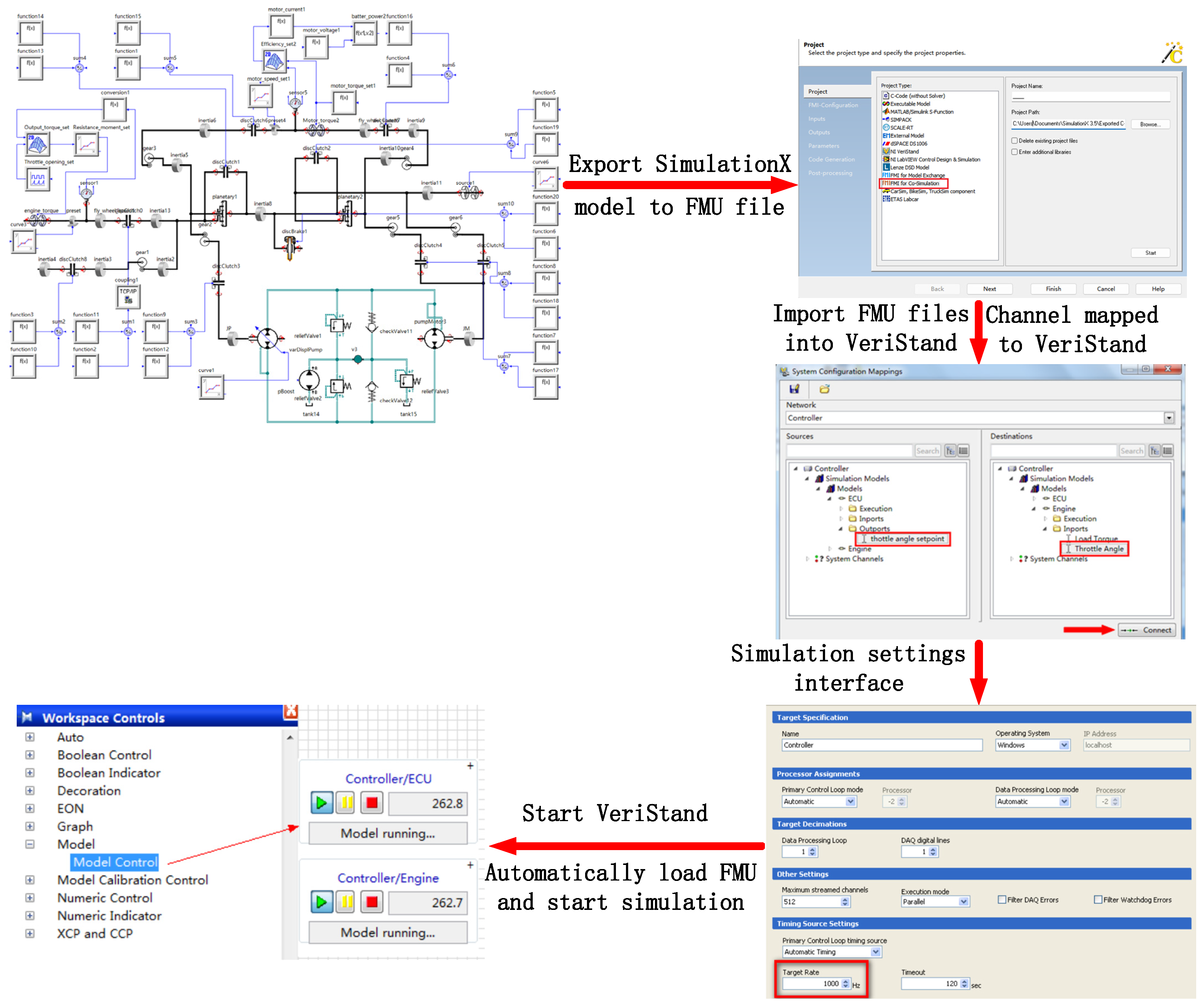
The MIL test process is shown in Figure 20. In this study, the SimulationX 3.5 and NI VeriStand 2018 software were used to build the MIL test platform. In the SimulationX model, the engine speed, torque, and clutch hydraulic control module are determined as input variables, and the output shaft speed, torque, and impact are determined as output variables. FMU (Functional Mock-up Unit) files can be exported through “FMI for co-Simulation” which is provided by SimulationX. In the VeriStand project, you can add “System Explore” and select the FMU file. VeriStand will automatically identify the variables in the FMU file and map the variables to VeriStand’s channels. In the simulation setting interface of VeriStand, you can configure parameters such as the simulation step size and target rate of FMU. After you start the VeriStand project, VeriStand automatically loads the FMU file and starts the simulation; VeriStand periodically reads the output variables of the FMU and sends the control instructions to the FMU [22].
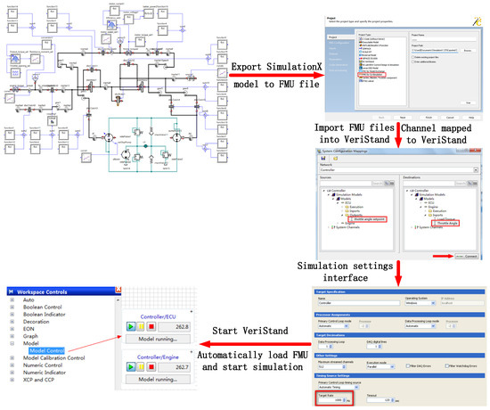
Figure 20.
MIL test scheme.
4.2. Variance Analysis of MIL Simulation Results
Model-in-the-loop (MIL) testing plays a crucial role in research, providing the dual guarantee of early validation of the development process and risk reduction. MIL testing can verify the accuracy of SimulationX simulation models before hardware development is completed. Through early validation, potential issues can be identified and resolved, avoiding costly reworking in the later stages, significantly reducing development risks and shortening project cycles. The MIL test laid a solid foundation for subsequent hardware-in-the-loop (HIL) testing and final vehicle testing. Verifying the accuracy of the simulation model through MIL testing can improve the credibility of HIL simulation results, reduce the need for many actual vehicle tests, and thus save time and resources.
Model-in-the-loop testing is influenced by environmental factors including signal transmission delays and noise interference originating from system components. As such, there are some errors in the results obtained. Therefore, the results with errors were statistically verified through orthogonal variance analysis. Different from range analysis, variance analysis requires arranging blank columns or conducting repeated tests [23].
Due to the interaction between factors, if a blank column is used, the model error will exaggerate the experimental error and mask the significance of the factor. The error caused by the interaction can be reduced by using the L16(24) orthogonal table for 16 MIL tests and two repeated tests. The results were averaged and analyzed using the MINITAB software.
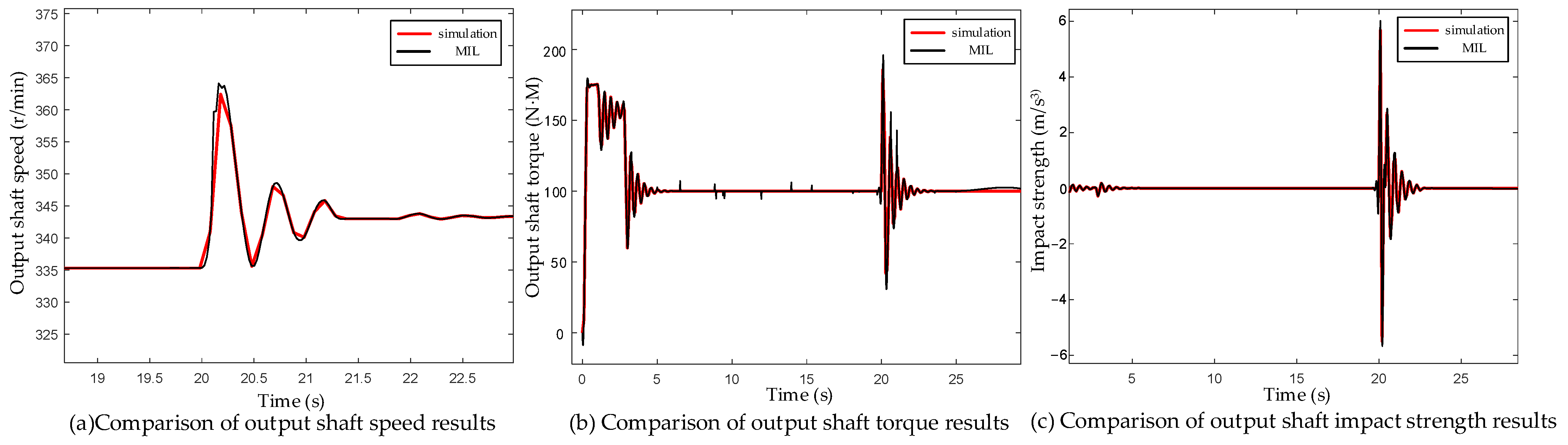
The optimal results of the MIL test were compared with the optimal results of simulation, as shown in Figure 21. The trend in the MIL test results is the same as that in the simulation results. The results from the MIL test were analyzed using variance analysis, and the findings are presented in the following table.

Figure 21.
Comparison of simulation and MIL results.
As presented in Table 8, variance analysis was conducted on the test results. The * in the table represents the magnitude of significance, and the more *, the higher the significance. The analysis revealed that factor A exerts the most significant influence on the output shaft’s velocity drop amplitude, factor D has a medium influence on the velocity drop amplitude of the output shaft, and factor B and factor C have no obvious influence on the velocity drop amplitude of the output shaft.
Table 8.
Analysis of velocity drop amplitude using variance method.
Table 9 presents the variance analysis results for the test, revealing that factors A and D have the most pronounced influence on the output shaft’s dynamic load coefficient. Conversely, factors B and C exhibit no discernable impact on this coefficient.
Table 9.
Analysis of dynamic load coefficient using variance method.
Table 10 presents the variance analysis of the test results, demonstrating that factor C exerts the most substantial impact on output shaft impact strength. Factor D exhibits a moderate impact, while factors A and B show no significant influence on output shaft impact strength.
Table 10.
Analysis of impact strength using variance method.
As demonstrated in Table 11, variance analysis was conducted on the test results. The analysis revealed that factor A exerts the most significant influence on switching time, while factors D, C, and B show no discernible impact.
Table 11.
Analysis of switching time using variance method.
A comparison and analysis of the simulation results and test results, as presented in Table 8, Table 9, Table 10 and Table 11, are summarized in Table 12.
Table 12.
Comparative analysis of simulation results and MIL test results.
The simulation results indicate that clutches C1 and C5 exert the most significant influence on the output shaft’s velocity drop amplitude. The test results demonstrate a high level of significance for clutch C1 and a moderate level for clutch C5; the simulation results show that both C1 and C5 have the most substantial impact on the output shaft’s dynamic load coefficient, and the test results confirm this with a high level of significance for both clutches. The simulation results indicate that clutches C4 and C5 exert the most significant impact on the output shaft impact strength. However, the test results show that the significance of these clutches is normal. The simulations suggest that clutches C1 and C5 have the greatest influence on switching time. The test results show that clutch C1 has a moderate level of significance, while clutch C5 shows no significant influence.
The test results indicate that the switching time is largely concentrated around 1.5 s, with minimal variation between individual tests. Consequently, the significance of each factor on the switching time is low. While some discrepancies exist between the simulation and test results, the overall trends are generally consistent. These discrepancies could stem from the omission of certain secondary factors during the simulation modeling process, as well as inherent errors present in the testing procedures.
5. Conclusions
Aimed towards optimizing the configuration of a hybrid tractor loaded with HMCVT, this paper focuses on the research and analysis of hydraulic mode and mechanical hydraulic transmission mode. Based on bench test data, the interpolation modeling method was applied to establish a theoretical model of an engine. The system simulation model was developed using the SimulationX software.
The following were chosen as evaluation metrics for mode switching quality: output shaft velocity drop amplitude, dynamic load coefficient, impact strength, and switching time. We optimized the quality of the switching process between the hydraulic mode and the mechanical hydraulic mode. The mode switching involves four interacting clutches. The orthogonal test was carried out using the L16(215) orthogonal table. The simulation results indicate that the A1D1C1B2 configuration provides the optimal comprehensive horizontal scheme. This entails switching clutches C1, C2, and C4 0.5 s ahead of schedule, while clutch C5 is engaged on time. This strategy achieves a reduction in the output shaft’s velocity drop amplitude from 17.647% to 6.591%, representing a 62.7% improvement. The dynamic load coefficient is also minimized, decreasing from 2.743 to 1.857, resulting in a 32.3% optimization range. The impact of the output shaft has been reduced from 14.125 to 5.67 m/s3, with an optimization range of 59.9%. Switch time has been reduced from 2.13 to 1.71 s. with an optimization range of 19.7%.
We established a model-in-the-loop test platform and designed an MIL test scheme. The enclosed test cabinet and the upper unit formed the physical part of the model-in-the-loop test. The whole-machine model constructed using SimulationX iwass transformed into dll files, which were then integrated into NI VeriStand for utilization. The test results were analyzed using the variance method. The experimental outcomes were juxtaposed with the simulation findings. The results show that there are some errors in the main factors affecting the velocity drop amplitude, dynamic load coefficient, and impact strength of the output shaft. This is caused by the error in the MIL test results. The effect of this on the switching time is small. This is because the switching time in the MIL test was mostly concentrated at about 1.5 s. There was little difference between the test results, so the significance of each factor was low.
The optimization method proposed in this study significantly improves the quality of clutch mode switching and effectively reduces the fluctuation in the transmission system. This achievement provides a key piece of technology for achieving smoother, more efficient, and reliable mode switching in hybrid mechanical hydraulic composite transmission systems. The effectiveness of this method was verified through MIL testing, demonstrating its feasibility for practical application and laying a solid foundation for subsequent research and development.
In the study of mode switching in this article, the friction coefficient of the clutch and the damping and dynamics of the transmission system between planetary gear mechanisms were not considered in the simulation modeling. The accuracy and completeness of simulation modeling for the clutch and planetary gear mechanisms should be improved in subsequent research.
This article focused on the verification of simulation results and only conducted a comparative analysis of the results through MIL experiments. Subsequent research will conduct a dynamic analysis of the entire vehicle transmission system, as well as parameter matching of the entire vehicle and its components, and establish a complete tractor bench test for further research and development.
Author Contributions
Conceptualization, Z.Z. and J.S.; methodology, J.S.; software, J.S.; validation, H.Z., D.W. and L.C.; formal analysis, L.C.; investigation, H.Z.; resources, Z.Z. and J.S.; data curation, Z.Z. and J.S.; writing—original draft preparation, Z.Z. and J.S.; writing—review and editing, Z.Z. and J.S.; visualization, Z.Z. and J.S.; supervision, L.C.; project administration, L.C., H.Z. and L.C.; funding acquisition, Z.Z., H.Z., D.W. and L.C. All authors have read and agreed to the published version of the manuscript.
Funding
This research was funded by the Open Foundation of the National Key Laboratory of Special Vehicle Design and Manufacturing Integration Technology (GZ2023KF007), the Open Foundation of the State Key Laboratory of Fluid Power and Mechatronic Systems (GZKF-202214), the China Postdoctoral Science Foundation (2023M731370), the National Natural Science Foundation of China (52272435, 52225212).
Institutional Review Board Statement
Not applicable.
Informed Consent Statement
Not applicable.
Data Availability Statement
The authors do not have permission to share data.
Conflicts of Interest
The authors declared no potential conflicts of interest.
References
- Sims, B.; Kienzle, J. Making mechanization accessible to smallholder farmers in sub-saharan Africa. Environments 2016, 3, 11. [Google Scholar] [CrossRef]
- Haini, H. The evolution of China’s modern economy and its implications on future growth. Post-Communist Econ. 2021, 33, 795–819. [Google Scholar] [CrossRef]
- Diao, X.; Silver, J.; Takeshima, H. Agricultural Mechanization and Agricultural Transformation; International Food Policy Research Institute: Washington, DC, USA, 2016; Volume 1527. [Google Scholar]
- Zhao, J.; Xiao, M.H.; Bartos, P.; Bohata, A. Dynamic engagement characteristics of wet clutch based on hydro-mechanical continuously variable transmission. J. Cent. South Univ. 2021, 28, 1377–1389. [Google Scholar] [CrossRef]
- Chen, X.; Zhao, Y.; Liu, K.; Wang, G.; Song, Y.; Chakrabarti, P. Shifting quality analysis of unmanned tractor equipped with series hydro-mechanical transmission. Trans. Can. Soc. Mech. Eng. 2024. [Google Scholar] [CrossRef]
- Yu, J.; Chen, H.; Liu, J. Speed ratio follow-up control of HMCVT based on variable universe fuzzy PID. China Mech. Eng. 2019, 30, 1226. [Google Scholar]
- Li, J.; Dong, H.; Han, B.; Zhang, Y.; Zhu, Z. Designing comprehensive shifting control strategy of hydro-mechanical continuously variable transmission. Appl. Sci. 2022, 12, 5716. [Google Scholar] [CrossRef]
- Zhao, X.; Ni, X.; Wang, Q.; Bao, M.; Li, S.; Han, S. Research on adaptive control strategy of hydraulic mechanical continuously variable transmission of a cotton picker. Proc. Inst. Mech. Eng. Part C J. Mech. Eng. Sci. 2020, 234, 3335–3345. [Google Scholar] [CrossRef]
- Lu, K.; Wang, L.; Lu, Z.; Zhou, H.; Qian, J.; Zhao, Y. Sliding Mode Control for HMCVT Shifting Clutch Pressure Tracking Based on Expanded Observer. Trans. Chin. Soc. Agric. Mach. 2022, 54, 410–418. [Google Scholar]
- Cheng, Z.; Lu, Z. Research on HMCVT parameter design optimization based on the service characteristics of agricultural machinery in the whole life cycle. Machines 2023, 11, 596. [Google Scholar] [CrossRef]
- Wei, X.; Wang, L.; Ni, X.; Han, S.; Zhao, X.; Li, S. Speed control strategy for pump-motor hydraulic transmission subsystem in hydro-mechanical continuously variable transmission. J. Mech. Sci. Technol. 2021, 35, 5665–5679. [Google Scholar] [CrossRef]
- Wang, G.; Song, Y.; Wang, J.; Xiao, M.; Cao, Y.; Chen, W.; Wang, J. Shift quality of tractors fitted with hydrostatic power split CVT during starting. Biosyst. Eng. 2020, 196, 183–201. [Google Scholar] [CrossRef]
- Xia, G.; Xia, Y.; Tang, X.; Zhao, L.; Sun, B. Speed regulation control of tractors’ new dual-flow transmission system based on slip rate resistance classification. Proc. Inst. Mech. Eng. Part D J. Automob. Eng. 2021, 235, 3571–3593. [Google Scholar] [CrossRef]
- Golovan, A.; Gritsuk, I.; Popeliuk, V.; Sherstyuk, O.; Honcharuk, I.; Symonenko, R.; Saravas, V.; Volodarets, M.; Ahieiev, M.; Pohorletskyi, D.; et al. Features of Mathematical Modeling in the Problems of Determining the Power of a Turbocharged Engine According to the Characteristics of the Turbocharger. SAE Int. J. Engines 2020, 13, 5–16. [Google Scholar] [CrossRef]
- Gharaibeh, K.; Costall, A.W. A Flow and Loading Coefficient-Based Compressor Map Interpolation Technique for Improved Accuracy of Turbocharged Engine Simulations; No. 2017-24-0023; SAE Technical Paper; SAE International: Warrendale, PA, USA, 2017. [Google Scholar]
- Maleev, R.A.; Zuev, S.M.; Fironov, A.M.; Volchkov, N.A.; Skvortsov, A.A. The Starting Processes of a Car Engine Using Capacitive Energy Storages. Period. Tche Quim. 2019, 16, 877–888. [Google Scholar] [CrossRef]
- Li, W.; Abel, A.; Todtermuschke, K.; Zhang, T. Hybrid vehicle power transmission modeling and simulation with simulationX. In Proceedings of the 2007 International Conference on Mechatronics and Automation, Harbin, China, 5–8 August 2007; pp. 1710–1717. [Google Scholar]
- Bao, M.; Ni, X.; Zhao, X.; Li, S. Research on the HMCVT gear shifting smoothness of the four-speed self-propelled cotton picker. Mech. Sci. 2020, 11, 267–283. [Google Scholar] [CrossRef]
- Rong, C.-X.; Wang, Z.; Cao, Y.; Yang, Q.; Long, W. Orthogonal Test on the True Triaxial Mechanical Properties of Frozen Calcareous Clay and Analysis of Influencing Factors. Appl. Sci. 2022, 12, 8712. [Google Scholar] [CrossRef]
- Matinnejad, R.; Nejati, S.; Briand, L.; Bruckmann, T.; Poull, C. Automated model-in-the-loop testing of continuous controllers using search. In International Symposium on Search Based Software Engineering; Springer: Berlin/Heidelberg, Germany, 2013. [Google Scholar]
- Bruggner, D.; Hegde, A.; Acerbo, F.S.; Gulati, D.; Son, T.D. Model in the loop testing and validation of embedded autonomous driving algorithms. In Proceedings of the 2021 IEEE Intelligent Vehicles Symposium (IV), Nagoya, Japan, 11–17 July 2021; pp. 136–141. [Google Scholar]
- Čech, M.; Königsmarková, J.; Reitinger, J.; Balda, P. Novel tools for model-based control system design based on FMI/FMU standard with application in energetics. In Proceedings of the 2017 21st International Conference on Process Control (PC), Strbske Pleso, Slovakia, 6–9 June 2017; pp. 416–421. [Google Scholar]
- Su, L.; Zhang, J.; Wang, C.; Zhang, Y.; Li, Z.; Song, Y.; Jin, T.; Ma, Z. Identifying main factors of capacity fading in lithium ion cells using orthogonal design of experiments. Appl. Energy 2016, 163, 201–210. [Google Scholar] [CrossRef]


Disclaimer/Publisher’s Note: The statements, opinions and data contained in all publications are solely those of the individual author(s) and contributor(s) and not of MDPI and/or the editor(s). MDPI and/or the editor(s) disclaim responsibility for any injury to people or property resulting from any ideas, methods, instructions or products referred to in the content. |
© 2024 by the authors. Licensee MDPI, Basel, Switzerland. This article is an open access article distributed under the terms and conditions of the Creative Commons Attribution (CC BY) license (https://creativecommons.org/licenses/by/4.0/).