Optimization of Sensor Placement for Modal Testing Using Machine Learning

Featured Application

This study introduces an innovative approach for optimizing sensor placement in modal testing by applying machine learning with enhanced efficiency and precision.

Abstract

Modal testing is a common step in aerostructure design, serving to validate the predicted natural frequencies and mode shapes obtained through computational methods. The strategic placement of sensors during testing is crucial for accurately measuring the intended natural frequencies. However, conventional methodologies for sensor placement are often time-consuming and involve iterative processes. This study explores the potential of machine learning techniques to enhance sensor selection methodologies. Three machine learning-based approaches are introduced and assessed, and their efficiencies are compared with established techniques. The evaluation of these methodologies is conducted using a numerical model of a beam to simulate real-world scenarios. The results offer insights into the efficacy of machine learning in optimizing sensor placement, presenting an innovative perspective on enhancing the efficiency and precision of modal testing procedures in aerostructure design.

1. Introduction

Mechanical structures are subject to vibrations. These vibrations can be internal (such as engine vibration), external (such as turbulence), or a combination of both. Therefore, characterizing the behavior of a system under vibration or other dynamic forces is crucial to good engineering design and pivotal for the aerospace and automotive industries [1,2].

Although the accessibility and speed of modern computers and FEA solvers may seem to obviate the need for physical modal testing, the results are only as accurate as the model being tested [3]. The results of modal testing can be compared with those of the theoretical model and used to establish if the model accurately describes the structure being analyzed [1]. Additional uses of modal testing include creating mathematical models of structures for integration into other analyses or developing models for structural health monitoring [1].

Modal analysis can be conducted on data acquired in laboratory conditions or from data acquired while the structure is in regular use [4,5,6]. In modal testing, sensors placed on the structure being tested—typically accelerometers and/or strain gauges—are measured to record their response to an excitation. The input can be provided by a modal shaker—a device that takes a signal as an input and applies that signal to the structure under test—or a modal hammer, where an impact is made against the structure to represent an instantaneous excitation [4]. In more complex tests or for large structures, multiple modal shakers may be used to induce a measurable excitation in the structure [1]. The outputs of the sensors are then post-processed, with the exact methodology being dependent on the excitation signal. These data may then be analyzed using a frequency response function in order to derive the natural frequencies and mode shapes of the structure under assessment.

Placing the sensors on the structure must be done with care, as their placement can substantially influence the results of a modal test. Large numbers of sensors increase the cost of testing because of the equipment and labor required to set up the test. As modal testing is principally concerned with structural dynamics, an ideal sensor selection would result in the lowest number of sensors that allows each sensor’s contribution to the analysis to be greatest [7]. The goal of optimizing sensor placement is to determine the most information about the structure’s behavior while minimizing the required number of sensors [7].

In early modal testing, sensor placement relied on engineering judgment and institutional knowledge derived from the fundamentals of vibration [8]. Although this may still be used in certain situations, such as with a well-understood structure or for simple geometries, novel structures present difficulties for this approach. Additionally, tight timelines due to budget constraints or limited access to testing facilities reduce the time available to refine sensor placement during testing [3]. As such, determining an efficient methodology for sensor placement has real implications for increasing efficiency. As a result, several methodologies have been developed to assist engineers in determining appropriate sensor placement for modal testing and structural health monitoring.

In general, methods for optimal sensor placement can be divided into two broad categories: model-based methods and data-driven methods. Model-based methods define the placement of sensors based on information derived from a numerical model, such as a finite element model or a multi-body model. Specifically in modal testing, existing model-based methods used for sensor placement include the Effective Independence Method (EIM) and the Iterative Residual Kinetic Energy approach (IRKE) [9]. Other techniques, such as those using information entropy, have also been developed [4]. A brief overview of these techniques is provided in Section 2.

Data-driven sensor placement strategies have also been proposed to extract the oscillatory characteristic directly from experimental measurements without requiring the need of a numerical model [10,11,12,13]. Zhang at el. [10] proposed a sensor placement approach that relies on a repetition of in situ trial measurements on bridges with different sensor positioning in order to avoid the need to rely on finite element data. The measured in situ data are used to train a Recurrent Gaussian Process Regression until a sufficient number of sensors is identified. However, this approach requires multiple experimental trials of sensor configurations, which is a costly approach for complex and large systems such as aerospace structures. Similarly, Suryanarayana et al. [12] employed a data-driven approach for optimal sensor placement of a multi-zone building. Their method requires that experiments with a large number of sensors are initially completed to collect the data necessary to apply the sensor placement approach. These data-driven methods often rely on operational modal analysis to extract the modes of the system during operations. Sashittal et al. [13] applied data-driven sensor placement to the observation of fluid flows. To the authors’ knowledge, no data-driven methodologies have been proposed for modal analysis to date.

This paper proposes a non-iterative model-based approach for optimal sensor placement in modal testing. Finite element models are generally available for large aerospace structures and can, therefore, be used to identify the number and positioning of sensors in the structure. The approach is based on machine learning techniques to avoid the need for iteration.

Machine learning (ML) techniques are a promising approach for determining sensor placement in modal analysis. In supervised machine learning, an input dataset is provided consisting of both the input data and the output. In this case, the input would be data derived from a finite element model and the output would be the mode shapes and natural frequencies. Based on this information, the model is then trained to be able to predict outputs based on new input data. As many of the previously discussed methods for sensor placement are iterative approaches, the problem of solving for sensor placement seems to be one to which machine learning is well suited [14,15,16,17].

This paper presents a novel methodology for sensor placement in modal analysis using random forest techniques. An initial application of the proposed approach is discussed in Kelmar et al. [18]. The paper is organized as follows. First, a review of traditional methodologies currently used for sensor placement in modal analysis is presented. Then, the proposed machine learning approach is presented and validated for a vibrating beam. The results of the proposed approach are then compared with the results obtained using one of the traditional methodologies.

2. A Review of Traditional Sensor Placement Techniques for Modal Testing

Several methodologies have been developed to assist engineers in determining appropriate sensor placement for modal testing and structural health monitoring based on a finite element model. Some of the current existing methodologies include the Effective Independence Method (EIM), the Mass-Weighted Effective Independence Method (MEIM), and the Residual Kinetic Energy approach (RKE) [16,19]. These existing methods are based on the modal analysis characteristics of the undamped structural dynamic system, which are the solutions of the following real symmetric eigenvalue problem:

$$\mathit{K}\mathbf{\Phi }-\mathit{M}\mathbf{\Phi }\lambda =\mathbf{0}$$

(1)

where $\mathit{K}$ is the stiffness matrix of the structural system, $\mathit{M}$ is the mass matrix, $\mathbf{\Phi }$ is the matrix containing the eigenvectors (modes) of the system, and $\lambda$ is the eigenvalue of the system; each n-th eigenvalue ${\lambda }_n$ corresponds to the n-th natural frequency ${\omega }_n$ through ${\lambda }_n={\omega }_n^2$. Bold notation indicates a matrix or vector quantity.

When modes are normalized to unit modal mass, the orthogonality parameter $\mathit{O}\mathit{R}$ is defined as follows:

$$\mathit{O}\mathit{R}={\mathbf{\Phi }}^T\mathit{M}\mathbf{\Phi }=\mathit{I}$$

(2)

The kinetic and strain energy distributions for each n-th mode ($\mathit{K}{\mathit{E}}_n$ and $\mathit{S}{\mathit{E}}_n$, respectively) are the term-by-term products (operator ⨂ represents element-wise matrix multiplication):

$$\mathit{K}{\mathit{E}}_n=\left\{\mathit{M}{\mathbf{\Phi }}_n\right\}\otimes {\mathbf{\Phi }}_n$$

(3)

$$\mathit{S}{\mathit{E}}_n=\left\{\mathit{K}{\mathbf{\Phi }}_n\right\}\otimes {\mathbf{\Phi }}_n/{\lambda }_n$$

(4)

The sum of the kinetic and strain energy distributions for each n-th mode is always equal to 1 when the modes are mass normalized, such that

$$\mathit{K}{\mathit{E}}_{TOT n}=\sum _{\mathit{i}=\mathbf{1}}^{\mathit{D}\mathit{O}\mathit{F}}\mathit{K}{\mathit{E}}_{i,n}=\mathbf{1}$$

(5)

$$\mathit{S}{\mathit{E}}_{TOT n}=\sum _{\mathit{i}=\mathbf{1}}^{\mathit{D}\mathit{O}\mathit{F}}\mathit{S}{\mathit{E}}_{i,n}=\mathbf{1}$$

(6)

DOF stands for “degrees of freedom”.

2.1. Effective Independence Method (EIM)

The Effective Independence Method, also known as the effective independence algorithm, is one of the most popular sensor placement techniques, and it bases its analysis on the sum of the diagonal terms of the Fisher information matrix. The Fisher information matrix is constructed using the modal characteristics extracted by a finite element model. It is an iterative method that evaluates the contribution of all possible sensor locations (i.e., the nodes of the finite element method) to the linear independence of the mode shapes. Sensors with small contributions to the linear independence are progressively eliminated until the desired number of sensors remains. This final set of sensors maximizes the sum of the diagonal and the condition number of the Fisher information matrix.

The method begins with a set of target mode shapes that encompass the set of candidate sensor locations generally derived from an FE model of the structure under analysis [20,21]. The algorithm attempts to predict the independence of each node based on the expected measured mode shape, with higher values indicating increased independence [20]. For this method, it is necessary to know both the expected mode shape as well as the location of candidate sensors; therefore, it is well suited for use when a finite element model is available. The candidate locations are then ranked according to the algorithm, removing the lowest ranking sensor and recalculating. As potential locations are eliminated, the relative independence of the remaining solutions increases, and the process is repeated until the required number of sensor locations is reached.

One of the challenges of EIM is that the optimal number of sensors must be defined a priori, and the potential locations of the sensors must be available [22]. A very fine grid of the finite element model allows the user to analyze all the possible locations of sensors, but the method then becomes very time-consuming owing to the iterative nature of EIM. Some research also suggests that more optimal results may be produced compared with kinetic energy methods, although at the cost of less ability to measure unexpected modes [20,23]. Additionally, the EIM approach does not account for unknown modes that may occur in the real world but do not appear in FEA. At the same time, if there are specific modes in the FEA results that are of more interest, EIM can provide targeted sensor selection for those modes that may require fewer sensors than necessary to capture the full behavior of the structure.

The EIM is derived by Kammer et al. [23] and is based on the concept that each sensor output ${\mathit{u}}_s$ can be represented as a linear combination of the mode shapes of the system at a given sensor location ${\mathbf{\Phi }}_s$ through the target modal coordinates $\mathit{q}$:

$${\mathit{u}}_s={\mathbf{\Phi }}_s\mathit{q}$$

(7)

The mode shapes of the system are obtained using finite element analysis. Each row in matrix ${\mathbf{\Phi }}_s$ represents a possible sensor location, and each column is the corresponding mode shape.

The linear independence of the mode shapes is defined through the Modal Assurance Criteria ($\mathit{M}\mathit{A}\mathit{C}$), as follows:

$$\mathit{M}\mathit{A}\mathit{C}={\mathbf{\Phi }}^{\mathit{T}}\mathbf{\Phi }$$

(8)

which yields 1.0 on the diagonal when the modes are normalized as such.

An effective independence score $\mathit{E}\mathit{I}$ is calculated for each possible sensor location, using the reduced modal content of the numerical model.

$$\mathit{E}\mathit{I}={\mathbf{\Phi }}_s{\left({\mathbf{\Phi }}_s^T{\mathbf{\Phi }}_s\right)}^{-1}{\mathbf{\Phi }}_s^T$$

(9)

This diagonal vector $\mathit{E}\mathit{I}$ yields a value that ranges between 0 and 1. A row with a value close to zero indicates that the sensor location is not able to sense the target modes, whereas a value close to one indicates that the sensor location is important to observe the target modes. The higher the effective independence score of a candidate sensor location, the more important that location is for calculating the independence of the mode shapes. Therefore, sensor locations with the lowest values are eliminated, and the effective independence score is then recalculated from the subset of candidate locations.

The lowest ranking row of $\mathit{E}\mathit{I}$ and the corresponding row in ${\mathbf{\Phi }}_s$ are eliminated, and the new ${\mathbf{\Phi }}_s$ is then input into Equation (2). Where the values of $\mathit{E}\mathit{I}$ are equal, either sensor location could be removed from the set of sensors without impacting the linear independence of the target modes.

The process is repeated until the desired number of sensors is reached. The sum of the column vector $\mathit{E}\mathit{f}\mathit{I}$ must always be equal to the number of target modes and, as a result, $\mathit{E}\mathit{f}\mathit{I}$ must be recomputed whenever a node is removed as irrelevant. As such, it is optimal to remove only one node per iteration. Additionally, it is impossible to have fewer sensors than target modes. The process is complete when the desired number of sensors is reached or when all remaining sensor locations have similar effective independence values [20].

The determinant of the Fisher information matrix ${\mathit{A}}_0$ is used to measure how much information is covered by a given sensor set:

$${\mathit{A}}_0={\mathbf{\Phi }}_s^T{\mathbf{\Phi }}_s$$

(10)

2.2. Mass-Weighted Effective Independence (MEIM)

A drawback to EIM is that it selects sensors by only considering the contribution to the linear independence of the mode shapes and neglects their orthogonality constraints through the mass matrix [24].

In fact, the $\mathit{M}\mathit{A}\mathit{C}$ matrix is generally not an identity matrix; therefore, it will not directly show the mode shapes to be linearly independent. As a consequence, the sensor locations selected by the effective independence method may not always be appropriate.

When a mass-weighted approach is used, such as the Mass-Weighted Effective Independence (MEIM), modes shapes that contribute the least to self-orthogonality are removed in each iteration as opposed to focusing purely on linear independence when selecting features. Cross-orthogonality checks are used to determine how analytical and empirical modal testing results correlate.

Based on Equation (11), a new Mass-Weighted Effective independence parameter is defined, such that

$$\mathit{M}\mathit{W}\mathit{E}\mathit{I}={\widehat{\mathit{M}}\mathbf{\Phi }}_s{\left({\mathbf{\Phi }}_s^T{\widehat{\mathit{M}}}^T{\widehat{\mathit{M}}\mathbf{\Phi }}_s\right)}^{-1}{\mathbf{\Phi }}_s^T{\widehat{\mathit{M}}}^T$$

(11)

where matrix $\widehat{\mathit{M}}$ is defined to allow $\mathit{M}={\widehat{\mathit{M}}}^T\widehat{\mathit{M}};$ therefore, $\widehat{\mathit{M}}={\mathit{M}}^{1/2}$.

One of the drawbacks, however, is that the Mass-Weighted Effective Independence requires the decomposition of the mass matrix to obtain $\widehat{\mathit{M}}$, which can be computationally prohibitive, as it requires the calculation of the eigenvalues and eigenvectors of the mass matrix $\mathit{M}$ or its Cholensky decomposition. The problem is reduced if the mass matrix $\mathit{M}$ is diagonal, and $\widehat{\mathit{M}}$ could then be found by taking the square root of all diagonal elements of $\mathit{M}$ [24].

2.3. Residual Kinetic Energy Method (RKE)

The RKE method is a technique that provides information on the sensor location that exhibits the maximum response for each mode shape and may offer improved performance over EIM. It is commonly used by NASA to determine sensor placement for modal testing based on detailed FEA models [25]. The method ensures that the residual kinetic energy is minimized in all degrees of freedom and modes under consideration. When this is computed, DOFs with high residual kinetic energy indicate that additional refinement is needed in order to measure the corresponding degree of freedom in a given mode. After another sensor is added to cover that degree of freedom, the residual kinetic energy is recomputed. This process is repeated until the solution is suitably orthogonal [26].

The RKE method ensures all recorded modes are fully orthogonal and, therefore, independent from each other.

The selection of the optimal sensor locations for modal testing using the RKE method is based on the partition of the modal vectors $\mathbf{\Phi }$

$$\mathbf{\Phi }=\left\{\begin{array}{c}{\mathbf{\Phi }}_s\\ {\mathbf{\Phi }}_o\end{array}\right\}$$

(12)

into ${\mathbf{\Phi }}_s$, which corresponds to “sensed” modal vectors (contains the DOF where sensors will be placed), and ${\mathbf{\Phi }}_o$, which corresponds to the “omitted” partition of the eigenvector (no sensor will be placed at these DOFs). The stiffness and mass matrix can also be partitioned accordingly, and Equation (1) becomes

$$\mathit{K}\mathbf{\Phi }-\mathit{M}\mathbf{\Phi }\lambda =\left[\begin{array}{cc}{\mathit{K}}_{ss}& {\mathit{K}}_{so}\\ {\mathit{K}}_{os}& {\mathit{K}}_{oo}\end{array}\right]\left\{\begin{array}{c}{\mathbf{\Phi }}_s\\ {\mathbf{\Phi }}_o\end{array}\right\}-\left[\begin{array}{cc}{\mathit{M}}_{ss}& {\mathit{M}}_{so}\\ {\mathit{M}}_{os}& {\mathit{M}}_{oo}\end{array}\right]\left\{\begin{array}{c}{\mathbf{\Phi }}_s\\ {\mathbf{\Phi }}_o\end{array}\right\}\lambda$$

(13)

A static Guyan reduction transformation is used to obtain an approximation of the omitted modes ${\mathbf{\Psi }}_o$:

$${\mathbf{\Psi }}_o=-{\mathit{K}}_{oo}^{-1}{\mathit{K}}_{os}{\mathbf{\Phi }}_s$$

(14)

The mass matrix corresponding to the selected sensor location is ${\tilde{\mathit{M}}}_{ss}$:

$${\tilde{\mathit{M}}}_{ss}={\left\{\begin{array}{c}\mathit{I}\\ {-\mathit{K}}_{oo}^{-1}{\mathit{K}}_{os}\end{array}\right\}}^{\mathit{T}}\left[\begin{array}{cc}{\mathit{M}}_{ss}& {\mathit{M}}_{so}\\ {\mathit{M}}_{os}& {\mathit{M}}_{oo}\end{array}\right]\left\{\begin{array}{c}\mathit{I}\\ {-\mathit{K}}_{oo}^{-1}{\mathit{K}}_{os}\end{array}\right\}$$

(15)

The orthogonality of the reduced modes identified using the selected points ${\mathbf{\Phi }}_s$ can be tested by parameter $\mathit{O}{\mathit{R}}_s$, which differ from the identity matrix because a reduced set of DOF is used to represent the modes:

$$\mathit{O}{\mathit{R}}_{\mathit{s}}={\mathbf{\Phi }}_s^T{\tilde{\mathit{M}}}_{ss}{\mathbf{\Phi }}_s \ne \mathit{I}$$

(16)

Industry and government standards require $\left|O{R}_{s, ij}\right|\le 10\%$ for $i\ne j$. The residual error can be defined as follows:

$$\mathit{R}=\left\{\begin{array}{c}{\mathbf{\Phi }}_s\\ {\mathbf{\Phi }}_o\end{array}\right\}-\left\{\begin{array}{c}{\mathbf{\Phi }}_s\\ {\mathbf{\Psi }}_o\end{array}\right\}=\left\{\begin{array}{c}0\\ {{\mathbf{\Phi }}_o-\mathbf{\Psi }}_o\end{array}\right\}=\left\{\begin{array}{c}0\\ {{\mathbf{\Phi }}_o+\mathit{K}}_{oo}^{-1}{\mathit{K}}_{os}{\mathbf{\Phi }}_s\end{array}\right\}$$

(17)

The error matrix is, therefore, a subtraction of the “omitted” DOF modes determined analytically (through finite elements or another analytical method) and the estimated “omitted” modes.

As the modal kinetic energy for the complete system is defined by Equation (3), a residual kinetic energy $\mathit{R}\mathit{K}\mathit{E}$ matrix can be defined using the residual error $\mathit{R}$:

$$\mathit{R}\mathit{K}\mathit{E}=\left(\mathit{M}\mathit{R}\right)\otimes \mathit{R}$$

(18)

Each column of the $\mathit{R}\mathit{K}\mathit{E}$ matrix represents the contribution of each degree of freedom to the residual kinetic energy of a specific mode. Similarly to $\mathit{R}$, the $\mathit{R}\mathit{K}\mathit{E}$ matrix is 0 at the rows corresponding to the sensor positions (measured DOF). The sum of the contribution of each degree of freedom is 1. Sensors should be placed at the locations of nodes with higher RKE values. The RKE matrix column will be much lower than 1 if that mode is already appropriately instrumented. By iterating through this matrix, the location where sensors should be placed can be determined, as well as the minimum number of sensor locations. This methodology works well when applied to existing analysis points to identify additional degrees of freedom that are under-measured by the initial sensor placement, and it has been adopted by NASA and others to meet NASA and Department of Defense standards for modal testing.

3. Machine Learning Approach for Sensor Selection

Machine learning (ML) techniques are a promising approach for determining sensor placement in modal analysis. Machine learning techniques are able to determine a non-deterministic relationship between an output quantity and a large number of input quantities—called “features”—on which the output depends, through an initial process called “training”. A large number of features are usually defined in a machine learning database, resulting in high computational costs. In an effort to reduce the computational costs of the training procedures and identify the most important factors that contribute to the desired output, several approaches have been defined to identify the most important features of the database. Examples of such approaches are the SelectKBest algorithm [27,28], the random forest feature importance approach [29,30], and Principal Component Analysis [31,32]. This paper focuses on the use of the random forest feature importance approach, as discussed in the following section.

The random forest (RF) feature selection approach was selected for sensor placement based on its promising performance in existing sensor selection applications [33]. The RF is a learning method for classification and regression that belongs to the CART family (CART: Classification and Regression Trees). It is considered an averaging ensemble method because it combines the results from multiple estimators and averages the predicted results to reduce variance.

During the training process, the random forest algorithm constructs a multitude of decision trees with a predicted estimation of the output variables; then, the outputs of all trees are aggregated, and the algorithm returns the average prediction of the individual decision trees. This aggregation process is called a bagging method, and it highly reduces the variance and the prediction bias—either underestimation or overestimation—of the output target, thereby reducing overfitting [29]. In addition to the randomness introduced by varying the input data for each DT, random perturbations in the DTs are also introduced. Each decision tree constructed by the algorithm is composed of internal nodes and leaves; in each internal node, all features are used to make decisions on how to binary split the dataset further based on a defined criterion, such as the Gini impurity or variance reduction parameters. This criterion measures how each feature decreases the impurity of the split at each node. For each feature, it is then possible to determine how, on average, it decreases the impurity of all trees in the forest, which becomes a measure of the feature importance [30]. In this paper, the Gini index will be used to determine the feature importance. Once the algorithm calculates the feature importance for each input variable, a bar graph can be obtained to determine the most important features. Additionally, the R squared value (R²) and mean squared error (MSE) can be used to evaluate the performance of the approach.

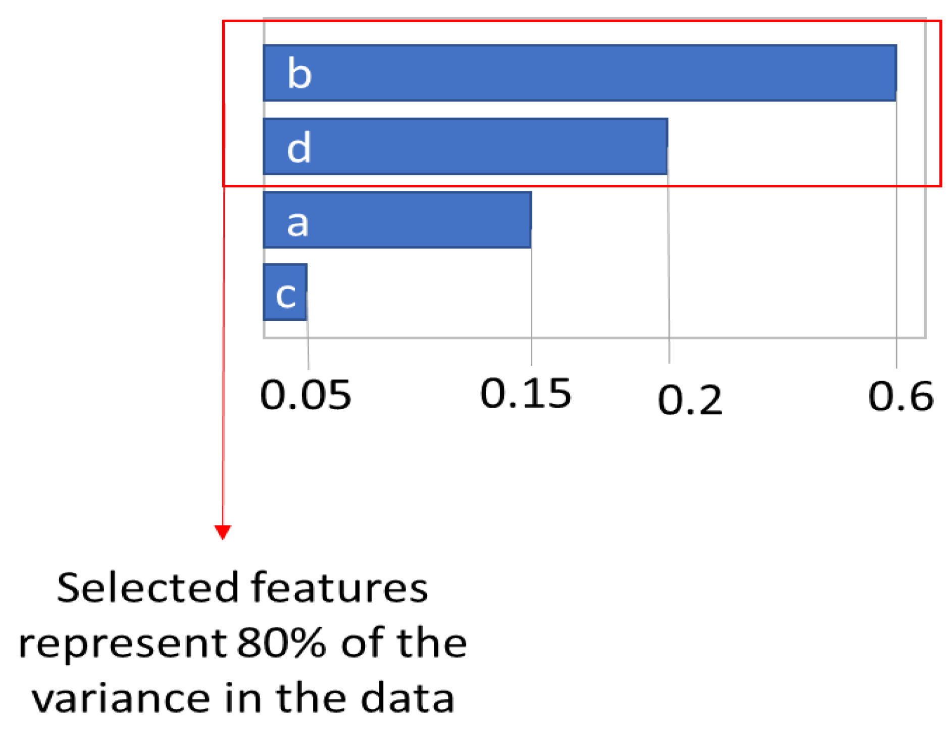
Initially, a random forest model is constructed using all the features available in the dataset. The random forest algorithm computes the feature importance of each input variable as it maps to the output variable. The regressor attributes a feature importance value that ranges between 0 and 1 to each input variable in the model. This value represents how much variance in the output is represented by each input variable. The sum of all feature importance of the model is 1. By selecting the inputs with the largest values of feature importance, we can determine which inputs are most valuable in representing the output. A number of inputs should be selected, such that a sufficient percentage of the variance of the data is represented.

Conceptually, if a model has four input variables called a, b, c, and d, the RF regressor attributes a feature importance value to each input. In Figure 1, input b has a feature importance of 0.6, input d has a feature importance of 0.2, input a has a feature importance of 0.15, and input c has a feature importance of 0.05. Therefore, input b is the most important feature and represents 60% of the variance in the data. Input d is the second most important feature and represents 20% of the variance in the data. Inputs b and d combined represent 80% of the variance in the data and could be used as a reduced model of the system.

This concept can be applied to sensor placement and selection by defining all the possible locations and types of sensors in the system as input variables [34]. The optimal number, location, and type of sensors are determined based on the most important features selected by the random forest regressor.

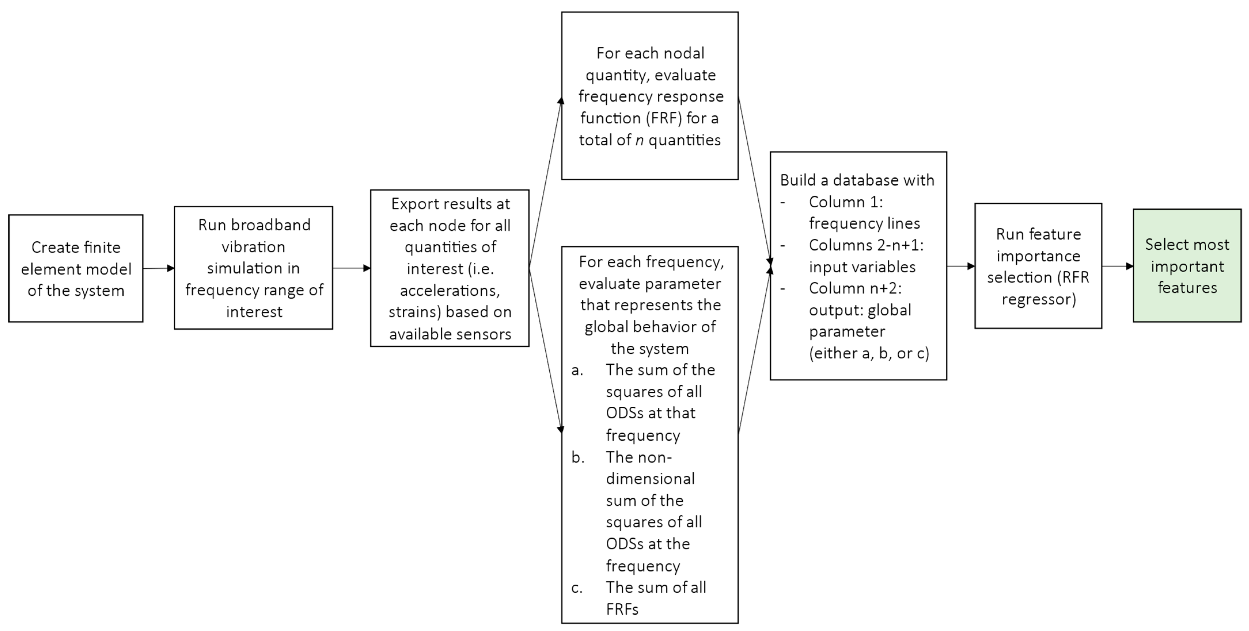
A flow-chart of the approach is shown in Figure 2.

First, a finite element (FE) model of the system is created, and a broadband time-domain simulation in the frequency domain of interest is performed. The results of the simulation are exported for each node and/or potential sensor locations. These locations must correspond to all the possible/viable locations for the sensors in the modal tests. All quantities corresponding to the desired sensors should be considered, such as strains, accelerations, etc. For each of these n locations and quantities, the frequency response function (FRF) is evaluated. FRF is defined as the ratio of the response (i.e., acceleration, velocity, or displacement) with respect to the excitation force, which is the reference. These quantities will be the inputs of the machine learning model.

Then, a scalar parameter that represents the global behavior of the system should be identified for each frequency at which the input FRFs are evaluated. This parameter will be used as output for the random forest feature importance approach.

Three different options for output parameters are evaluated in this paper: the raw Operational Deflection Shape (ODS), the normalized ODS, and the average FRF.

• Global parameter (a): raw ODS.

The sum of the squares of the ODS at each possible sensor location is evaluated according to

$$\mathrm{O}\mathrm{u}\mathrm{t}\mathrm{p}\mathrm{u}\mathrm{t} \mathrm{a}=OD{S}_{\omega }^{T}OD{S}_{\omega }$$

(19)

where $OD{S}_{\omega }$ contains the operational deformed shape at each frequency $\omega$. This expression results in a distinct scalar value for each ODS at each frequency.

Output a, however, depends on the load condition of the beam and will change depending on the magnitude of the load applied to the beam.

2.

Global parameter (b): normalized ODS.

To decrease the sensitivity of the output to the load conditions, a normalized form of output a is calculated as follows:

$$\mathrm{O}\mathrm{u}\mathrm{t}\mathrm{p}\mathrm{u}\mathrm{t} \mathrm{b}=\frac{OD{S}_{\omega }^{T}OD{S}_{\omega }}{{\left|OD{S}_{\omega }\right|}^2}$$

(20)

Dividing the ODS product by the magnitude of the ODS at that frequency reduces the effect of the external load on the output used by the random forest feature importance approach and, therefore, on the sensor placement.

3.

Global parameter (c): average FRF.

The last output chosen was the average FRF at a given frequency, where n is the number of nodes, and the sum of the FRF at a given frequency is taken across all nodes n.

$$\mathrm{O}\mathrm{u}\mathrm{t}\mathrm{p}\mathrm{u}\mathrm{t} \mathrm{c}=\frac{\sum FRF\left(f\right)}{n}$$

(21)

After all local and global quantities are evaluated, the database can be created according to

Table 1. Structure of th random forest feature importance dataset.

Freq (Hz)	Node 1	Node 2	…	Node n	Output
f	Node 1 FRF (f)	Node 2 FRF (f)		Node n FRF (f)	Output (f)

. The first column contains the frequency, columns 2 to (n + 1) contain the FRF at each desired location and represent the input variable, and the last column (n + 2) contains the global parameter and will be the output quantity for the random forest regressor. The random forest method can be run to obtain the ranking of the most important features, which can then be selected as the location and type of sensor needed for modal testing.

Dataset Creation

The dataset for the random forest regression model is extracted from a finite element model of the desired system and reformatted as specified in Table 1. Each row in the dataset corresponds to a frequency for which the FRF of each node is calculated. Each row in this case represents the operational deflection shape (ODS) for a given frequency for every node in the numerical modal model. The frequency is used primarily for tracking and is not input into the RF. The output column in this table represents the value the model should attempt to represent.

The model will output a table of all the input features (nodes) and their corresponding importance for predicting the output value. Therefore, choosing a parameter for the output is crucial to producing results that reflect an optimal sensor placement. All three global parameters will be considered as possible output parameters, and the resulting sensor placement will be presented in the next section.

4. Application of the Random Forest Sensor Selection Approach to a One-Dimensional Structure

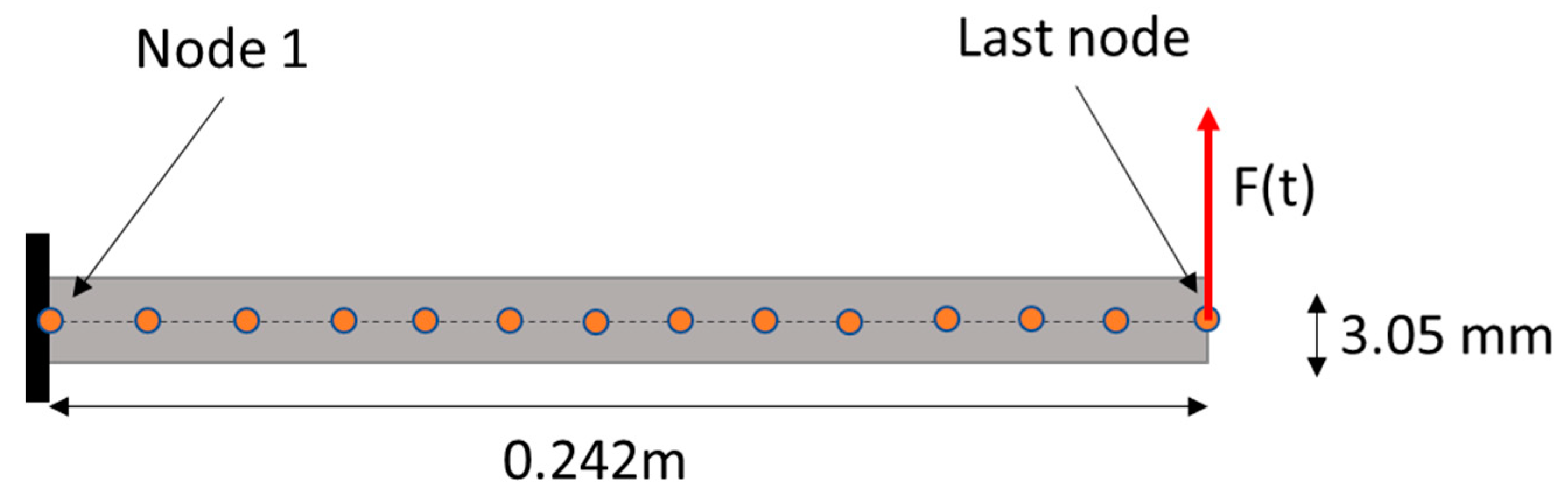
The proposed method is applied to the analysis of a cantilever aluminum beam, the properties of which are listed in

Table 2. Cantilever beam properties.

Property	Value
Length	0.242 m
Width	0.032 m
Thickness	0.00305 m
E (Young’s modulus)	70 GPa
$\upsilon$ (Poisson’s ratio)	0.33
$\rho$ (density)	2700 kg/m3

.

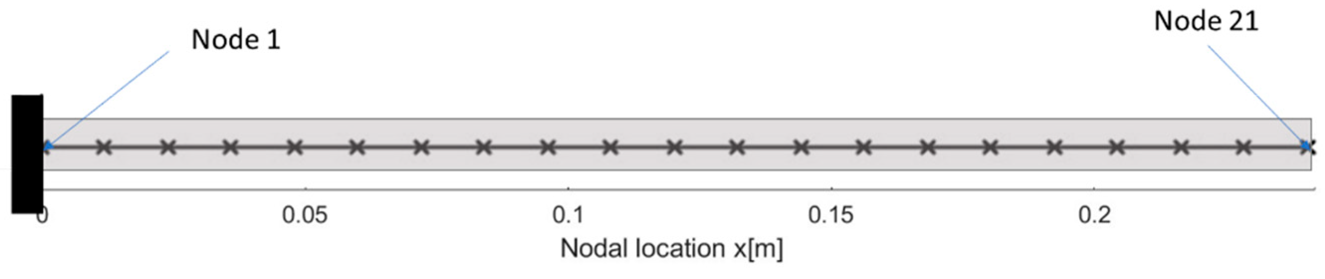
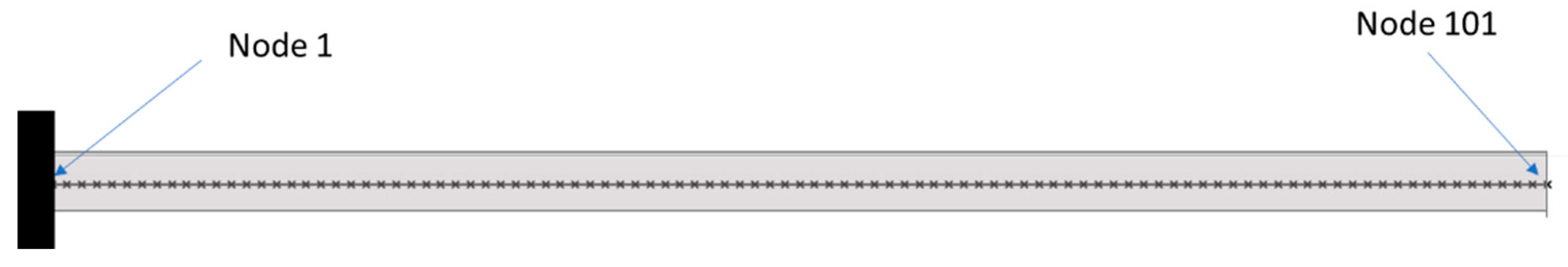
The transverse behavior of the beam is modeled using 1D Euler–Bernoulli beam elements. The beam is clamped on one side, corresponding to Node 1; a transverse time-varying load is applied at the free end of the beam, corresponding to Node n of the beam (Figure 3). The mesh of the beam is shown in Figure 4.

The first seven natural frequencies of the beam are listed in

Table 3. Natural frequencies of the cantilever beam.

Mode Number	FEA Natural Frequency (Hz)
1	42.83
2	268.26
3	750.45
4	1468.6
5	2423.4
6	3612.5
7	5033.1

.

In the first case, a fine mesh is considered (100 elements) for the RF analysis. A second case is presented, in which the number of elements composing the mesh of the beam is reduced to 20 elements. Comparison of these two cases will determine whether the method is sensitive to the mesh of the model. In the third case, the time history of the applied load is changed to determine the sensitivity of the approach to the loading condition.

4.1. Densely Meshed Cantilever Beam (Case 1)

For this first case, a finite element model of the cantilever beam was created using 100 linear beam elements, corresponding to an element size and distance between nodes of 2.4 mm. The beam was subjected to a transverse broadband Gaussian white-noise excitation from 0 Hz to 50 kHz, as shown in Figure 5, applied at the free end of the beam.

The database used by the RF feature importance approach was created from the transverse acceleration at each node. Transverse acceleration was chosen as the input parameter owing to the wide availability of linear accelerometers for modal testing.

In this first example, all three definitions of the global parameter are explored. For each output option, an RF model is trained using the available data. To understand the capability of the RF to represent the output, the R² and MSE are shown in

Table 4. R² and MSE of RFR for case 1.

	(a) ODS	(b) Normalized ODS	(c) Avg. FRF
R2	0.900	0.940	0.940
MSE	7.0 × 10−15	4.4 × 10−9	2.8 × 10−11

. The MSE and R² values in Table 4 appear excellent, giving confidence that the RF model is a good representation of the system and that the feature importance algorithm is reliable.

The ten most important features from each global parameter selection are listed in

Table 5. Most important sensor locations (nodes) for case 1 based on different selections of the global parameter.

Feature Importance Rank	(a) ODS	(b) Normalized ODS	(c) Avg. FRF
1	86	66	61
2	69	100	47
3	44	68	94
4	12	92	42
5	43	73	41
6	70	34	48
7	53	82	5
8	101	20	82
9	96	88	101
10	87	83	57

. These features represent the first ten candidate sensor locations identified by the RF algorithm. The nodal numbering starts with “node 1” at the root of the beam and ends with node 101 at the tip of the beam.

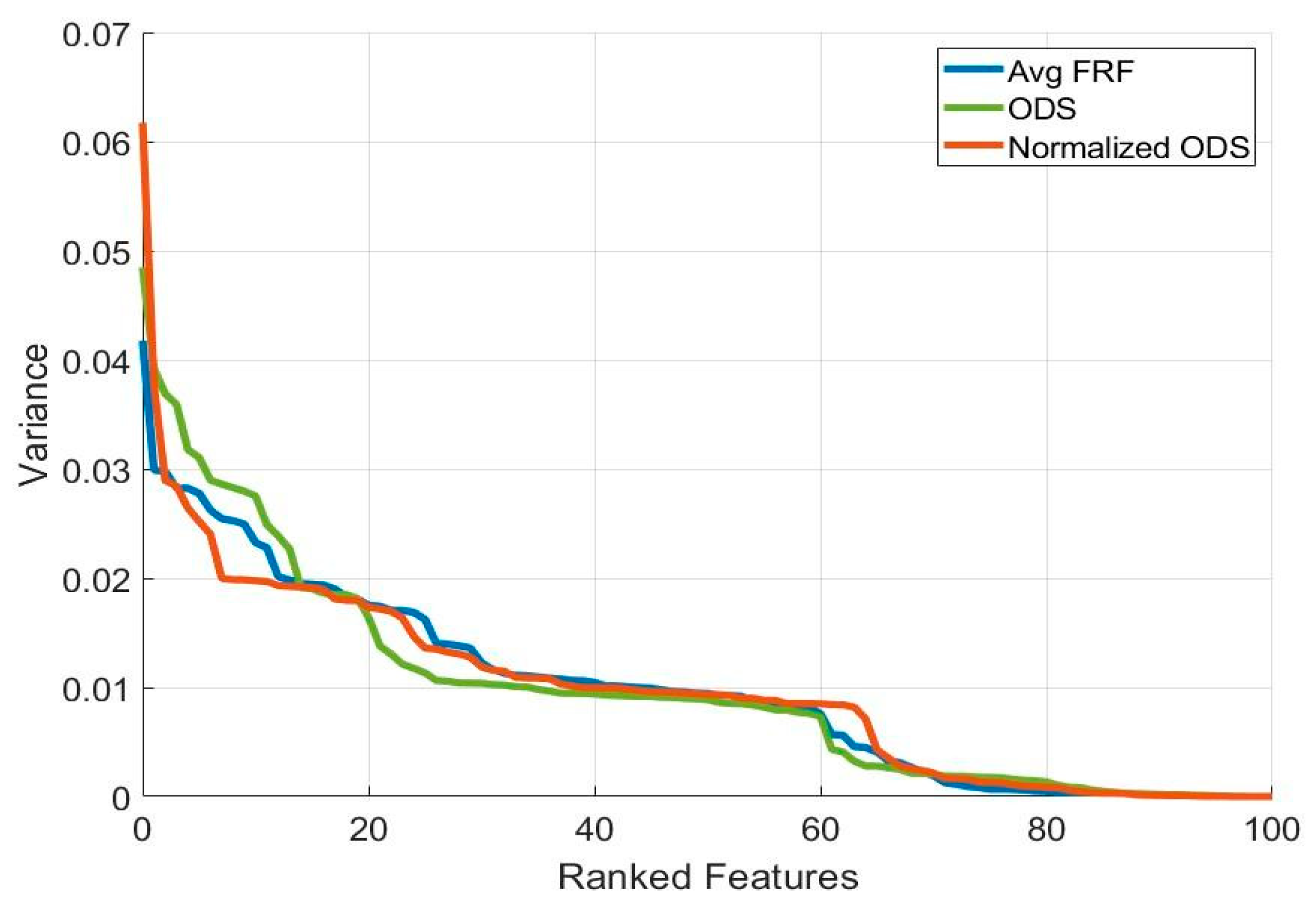
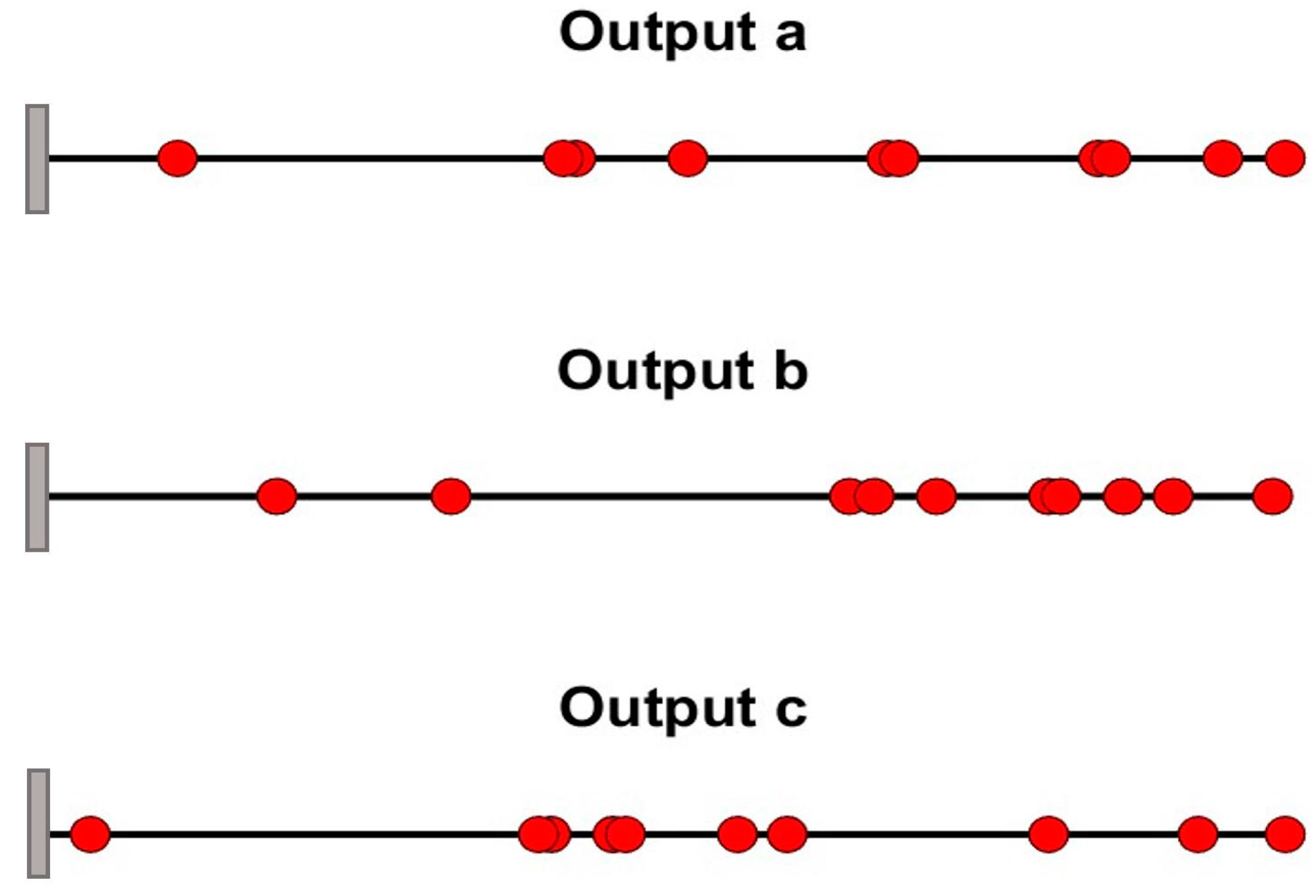
The contribution of each feature/sensor to the variance of the data is depicted in Figure 6. The first ten features of the ODS RF account for 31% of the variance (global parameter a), whereas the first ten features of the normalized ODS account for 34% of the variance (global parameter b) The first 10 features of the average FRF account for 29% of the variance (global parameter c). The position of the first ten sensors identified by the RF approach for the three outputs are depicted in Figure 7; some of the sensors are overlapping or very close to each other (e.g., 2.4 mm between sensor locations 43 and 44 for output a), which is not physically possible in a real testing environment.

For all three choices of output, approximately 20 features are needed before at least 50% of the variance is accounted for; however, output (a) exhibits slightly higher individual variance in the first three features.

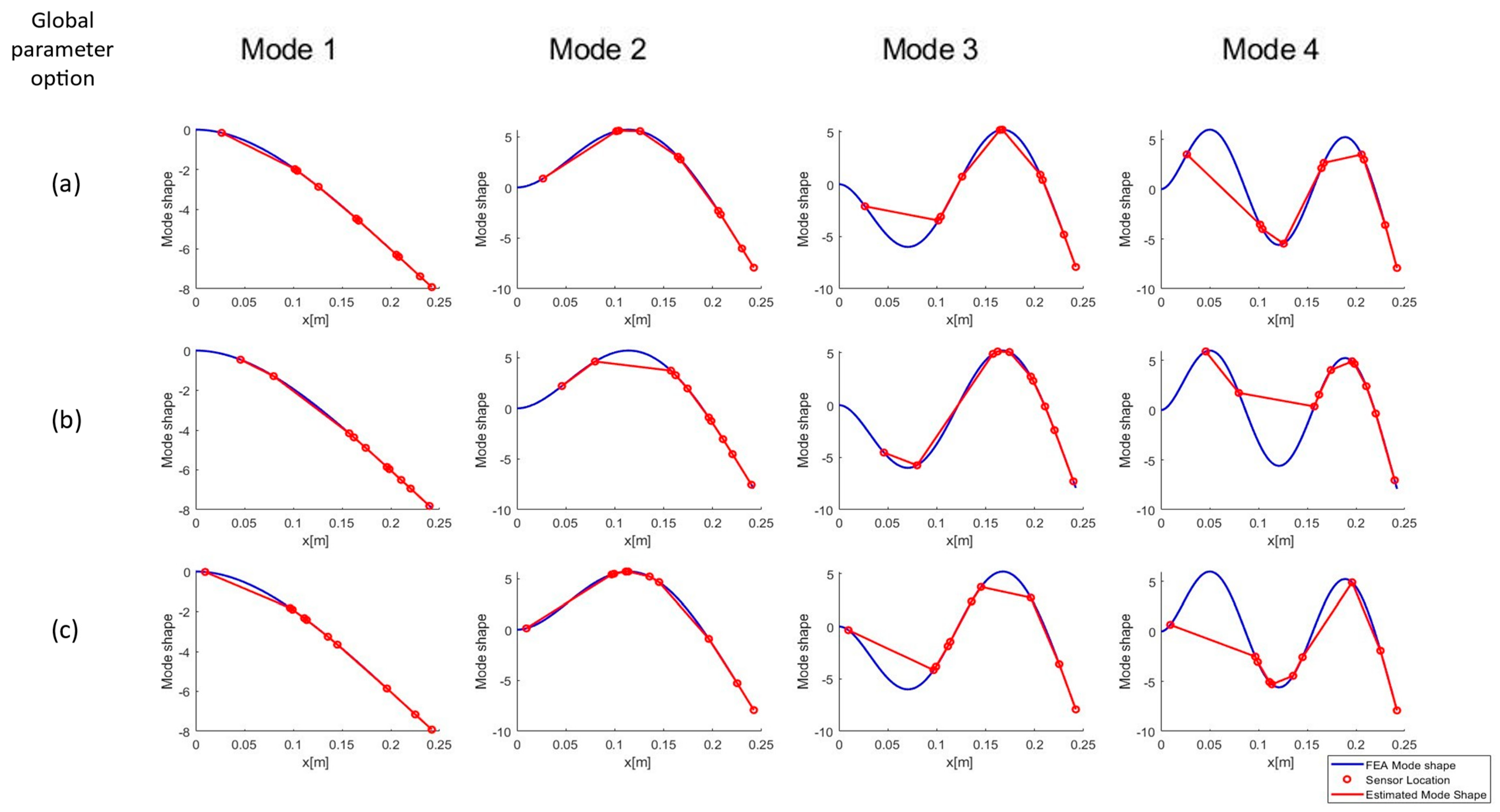
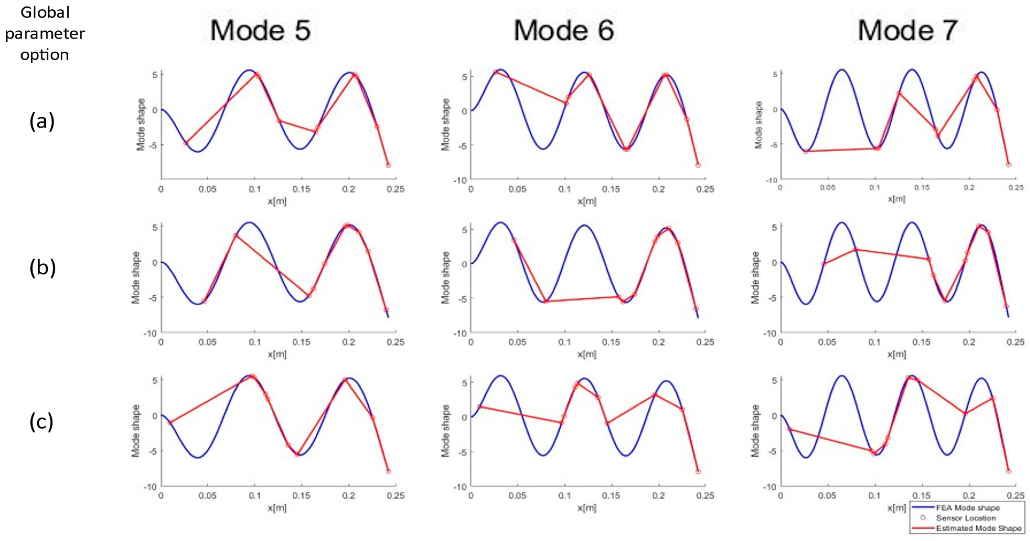
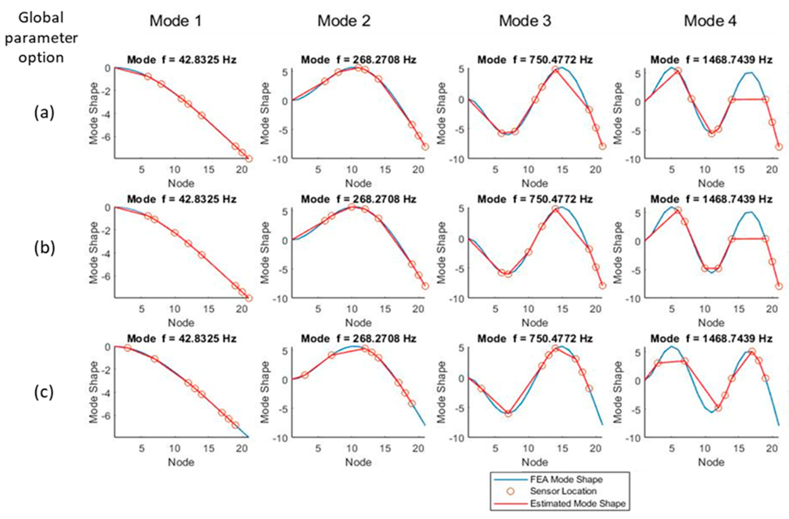
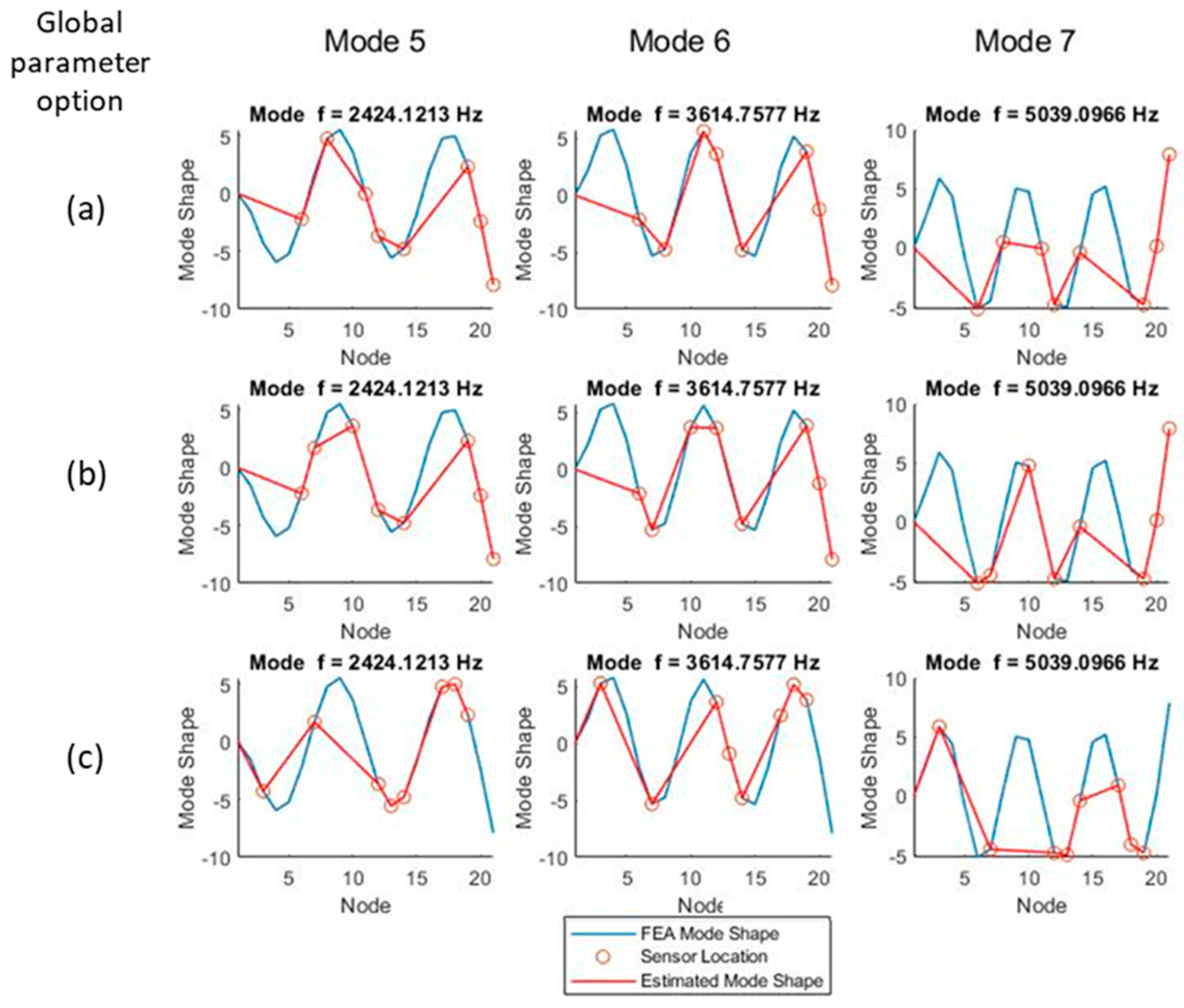
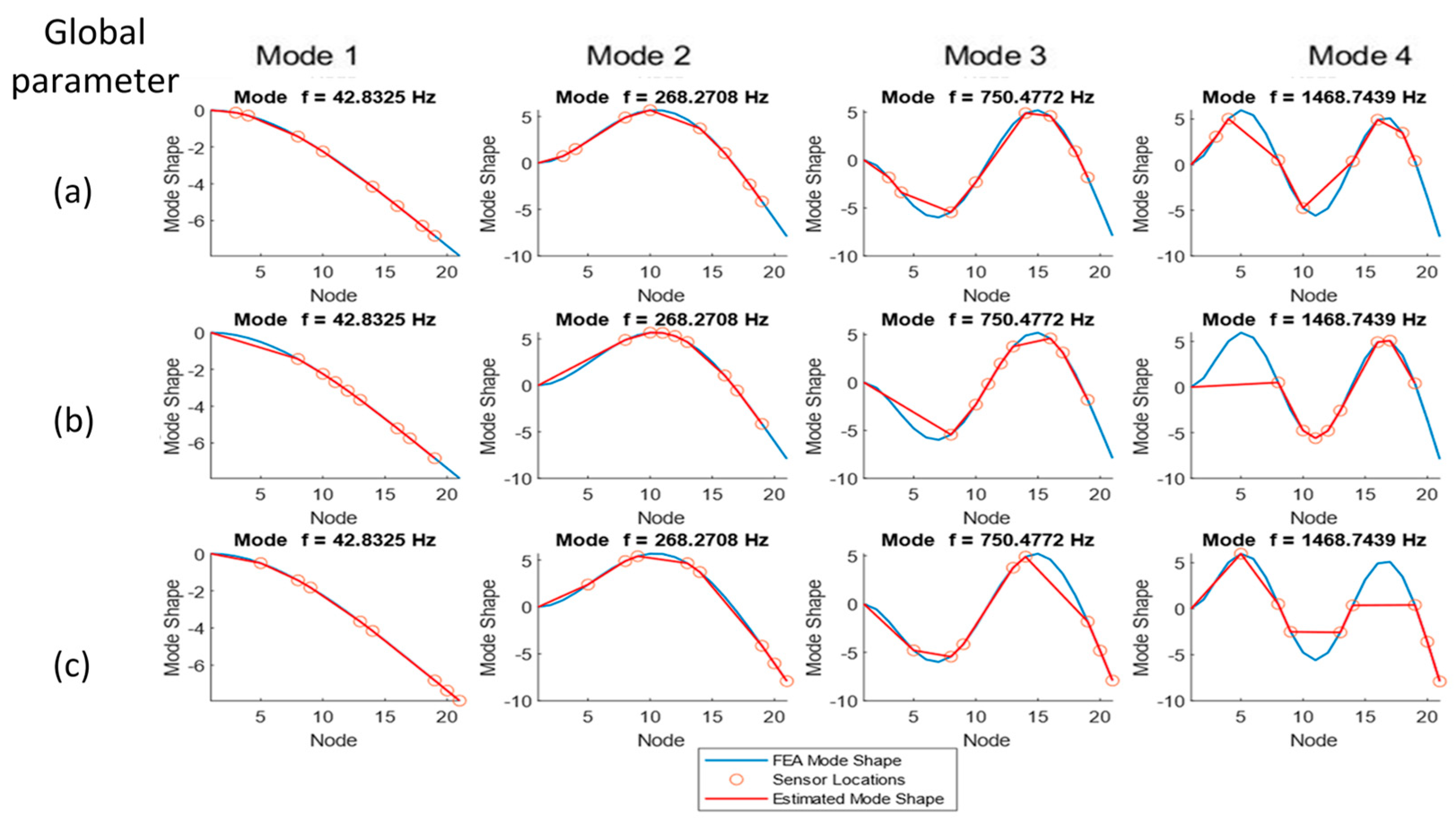
To estimate the mode shapes that the selected sensors will predict, the value of the actual (FEA) mode shape was taken at each candidate sensor location. To obtain the mode shapes in the figures, the numerical mode shapes were evaluated at the selected sensors’ locations to verify that minimum aliasing is present with the proposed choice. The mode shapes are depicted in Figure 8 (modes 1–4) and Figure 9 (modes 4–6). Each column in the charts represents a mode, and the rows display the different global parameter choices (a: raw ODS, b: normalized ODS, c: average FRF). Sensor locations do not vary between modes but are plotted on top of the different mode shapes to visually evaluate the ability of the sensors to measure a given mode shape.

All three sensor sets obtained using the different choices of output parameters can predict the first four modes with relative accuracy. Starting at mode 4, mode peak clipping can be noted with all global parameter options.

As the mode number increases (Figure 9) the predictions made using the machine learning modeling fail to capture the behavior of the first third of the beam, as all methods weight the free end of the beam more heavily. The method is able to capture the number of nodes for each mode and does not exhibit large aliasing errors in the representation of mode shapes. At mode 7 and above, the aliasing of the modes along the length of the beam starts to become apparent, which is expected with only ten sensor placements on the structure.

4.2. Effect of Mesh Density on Sensor Selection Using a Random Forest Regressor (Case 2)

The previous subsection defined optimal sensor locations for modal analysis with a mesh of 100 elements. This mesh results in an element size of 2.42 mm. Since the method allows for the placement of a sensor at any given node, it can select adjacent nodes for sensor placement (Figure 7 and Table 5). This distance between nodes (element size) is impractical for physical sensors. This subsection discusses the sensitivity of the approach to the mesh size.

For the second case, the mesh is reduced to 20 elements, resulting in minimum sensor distances of 12.1 mm, which is more reasonable, as shown in Figure 10. The rest of the parameters for the finite element and random forest analyses are the same as in case 1, including the applied excitation and the physical properties of the beam.

Table 6. Most important sensor locations for case 2, ranked by feature importance.

Feature Importance Rank	(a) ODS	(b) Normalized ODS	(c) Avg. FRF
1	12	20	14
2	11	21	13
3	20	14	19
4	8	19	7
5	19	12	12
6	21	7	17
7	14	6	18
8	6	10	3

lists the first eight positions selected as the best sensor locations by the RF feature importance applied to a coarser mesh. A nodal location of 1 corresponds to the root of the cantilever beam, and 21 corresponds to the tip of the beam.

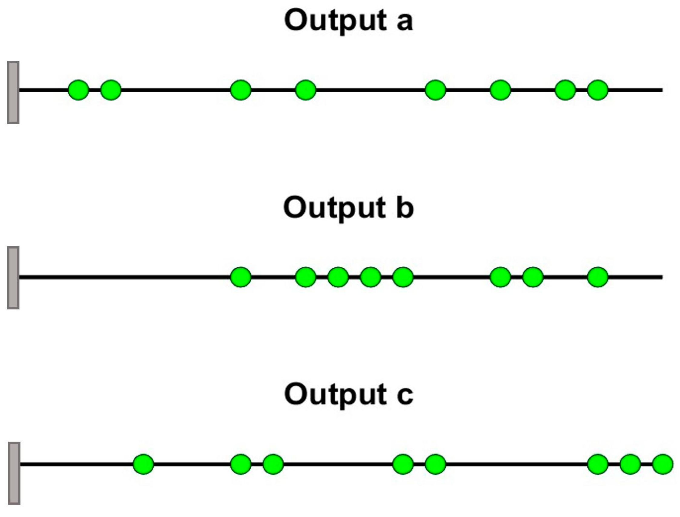
The first eight features of the ODS RF (global parameter a) account for 55% of the variance, which represents a considerable improvement compared with case 1. Similar changes pertain to the other two choices of global parameter: the first ten features of the normalized ODS RF (global parameter b) account for 56% of the variance, and the first eight features of the Avg. FRF RF (global parameter c) account for 52% of the variance. This improvement is expected, as the eight most important features in case 2 account for 40% of the total nodes, whereas in case 1 the 10 most important features account for only 10% of the total nodes.

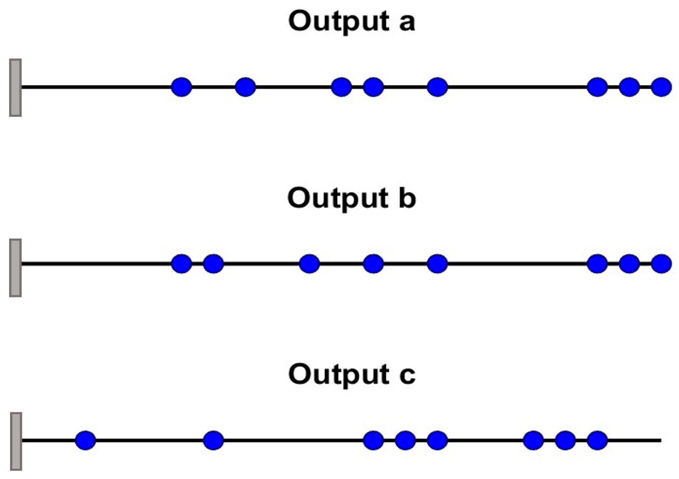
The positions of the first eight sensors identified by the RF approach for the three outputs are depicted in Figure 11. It is clear that the overlapping problems identified in case 1 have been eliminated.

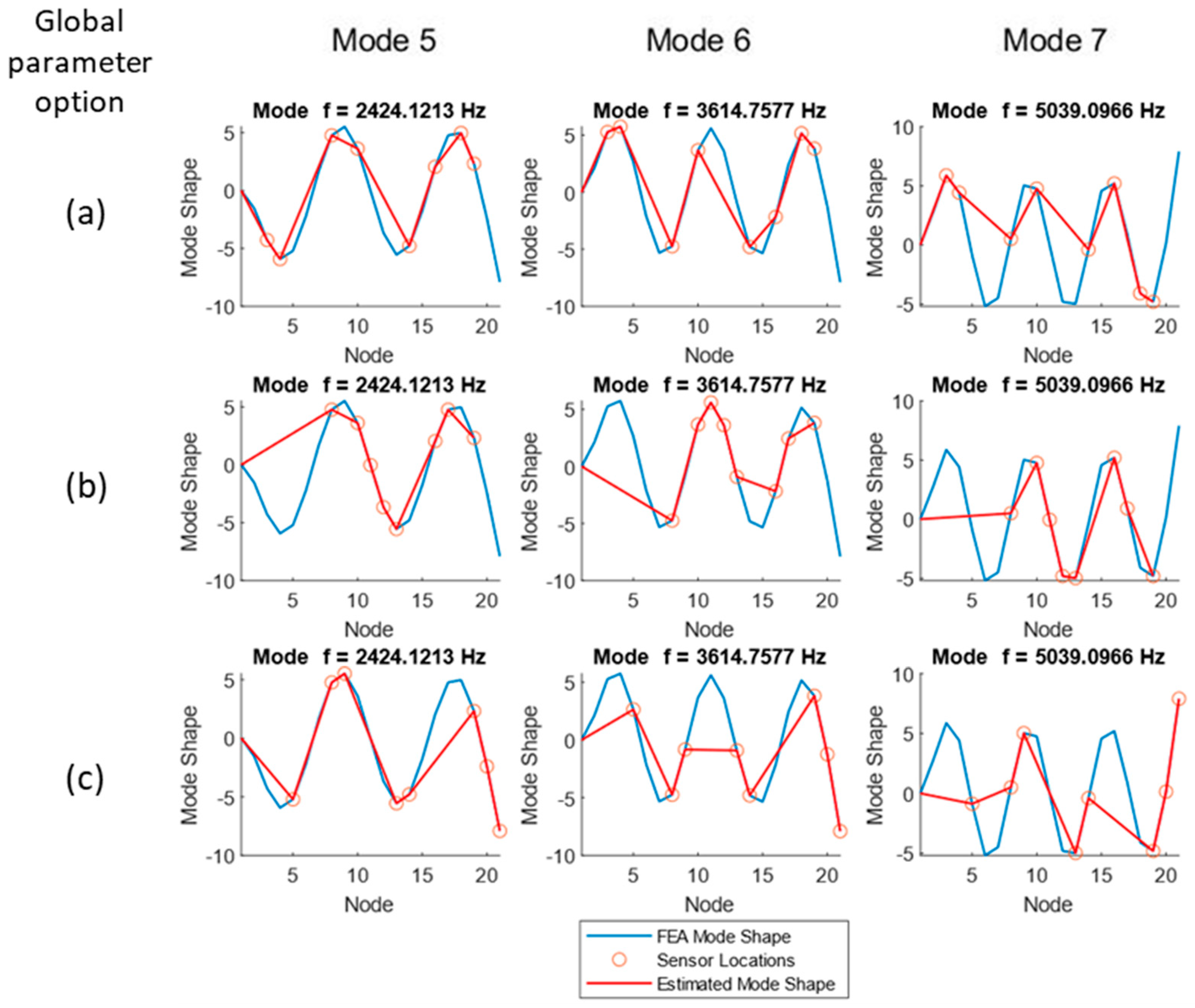
Visualizations of the ability of the sensors to identify the modes of the beam are depicted in Figure 12 and Figure 13. The plots were created using the same methodology as Figure 8 and Figure 9. Examining the plots, the ODS sensor selector (global parameter a) appears to perform worse, with almost all the sensors placed at inflection points for the 7th natural frequency.

Upon comparison of the figures of the modes of case 1 (Figure 7) and 2 (Figure 11), it can be seen that the selected sensor locations are similar for both cases, suggesting the robustness of the method according to mesh size. Comparing Figure 8 and Figure 9 with Figure 12 and Figure 13 shows that reducing the number of elements of the beam does not affect the accuracy of the proposed methods in representing the modal characteristics of the beam. The accuracy of the method is not reduced because 20 elements are sufficient to represent the modal content of the beam up to the considered natural frequency (the first seven bending modes).

The ability of the method to properly select sensor locations for modal testing is further verified by extracting natural frequencies from the selected FRF using a modal analysis procedure. The natural frequencies extracted by these signals using the Gaussian white-noise excitation are presented in

Table 7. Extracted natural frequencies, case 2.

	FEA	(a) ODS		(b) norm ODS		(c) Avg. FRF
Mode #	f (Hz)	f (Hz)	% Err	f (Hz)	% Err	f (Hz)	% Err
1	42.8	–	100%	54.3	27%	–	100%
2	268.3	277.5	3%	281.6	5%	278.0	4%
3	750.5	755.7	1%	757.5	1%	751.7	0%
4	1468.7	1471.0	0%	1462.8	0%	1462.6	0%
5	2424.1	2397.1	1%	2395.1	1%	2398.2	1%
6	3614.8	3526.0	2%	3531.6	2%	3499.3	3%
7	5039.1	4834.3	4%	4747.1	6%	–	–

. All choices for global output yield results that closely match the natural frequencies derived by the modal analysis of the finite element model; however, all sensor configurations are poor predictors of the first natural frequency, with the normalized ODS parameter performing better with an error of 27% (Table 7). In the mid-range frequencies, all three methods perform quite well, with errors below 6% from the numerical frequency.

4.3. Effect of Excitation Signals on Sensor Selection Using a Random Forest Regressor (Case 3)

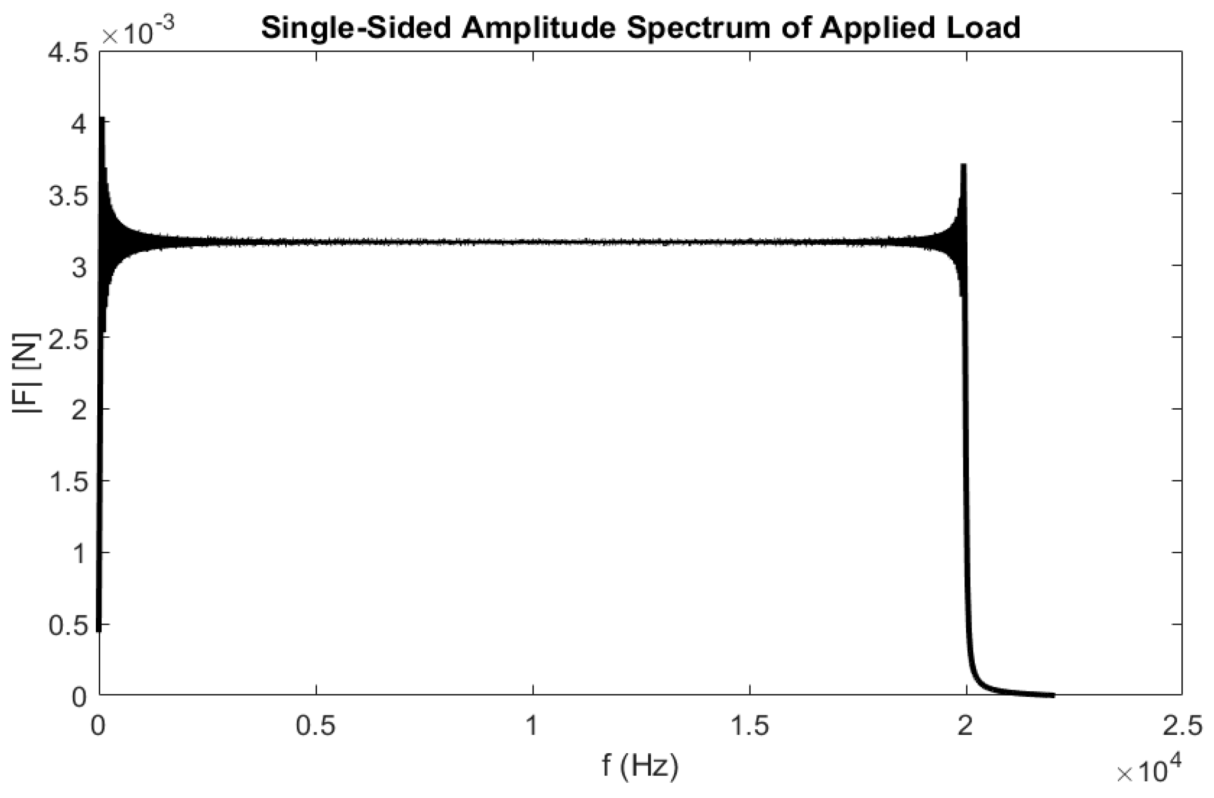
To study the effect that the choice of excitation signal has on sensor selection using the proposed methodology, two different excitation signals were chosen for comparison. Although traditional methods should select sensors for modal testing independently of the excitation signal, the random forest method is sensitive to the chosen excitation frequency due to how the input database is constructed. The first excitation consists of the Gaussian white-noise input signal used in the previous sections (cases 1 and 2), and the second excitation signal is a linear chirp, as described below (case 3). The comparison will be based on a mesh size of 20 elements identical to case 2.

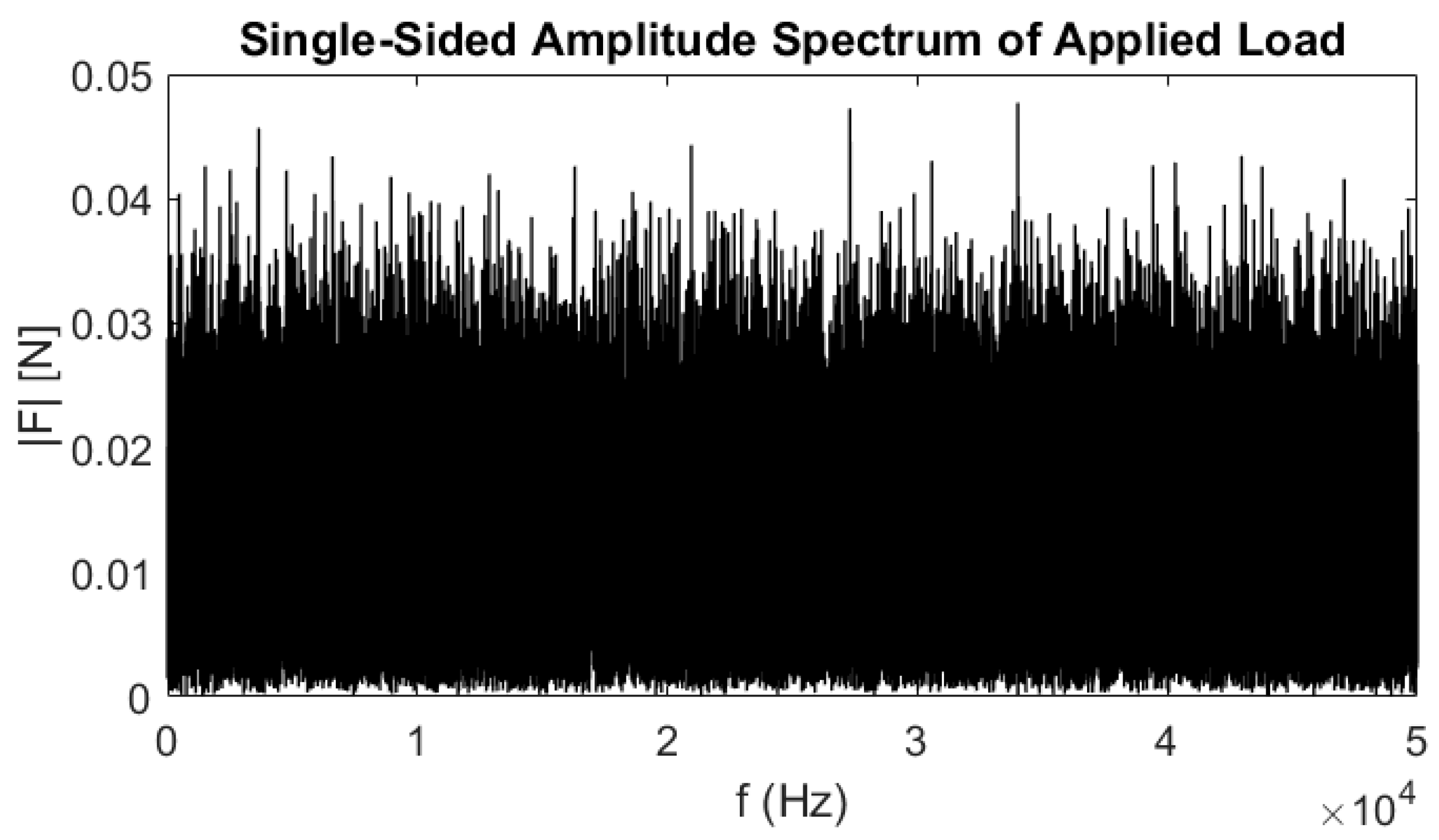
The beam was excited using a linear chirp signal, whose single-sided amplitude is depicted in Figure 14 as a function of frequency.

The same three global parameters were considered for this case. The sensors selected by the approach for this different excitation signal are listed in

Table 8. Most important sensor locations for case 3, ranked by feature importance.

Feature Importance Rank	(a) ODS	(b) Normalized ODS	(c) Avg. FRF
1	10	19	20
2	19	13	9
3	4	8	19
4	14	16	21
5	8	12	14
6	3	10	13
7	16	11	5
8	18	17	8

.

The positions of the first eight sensors identified by the RF approach for the three outputs are depicted in Figure 15.

To better visualize the locations of the sensors and the potential for the sensors to capture the desired mode shapes, each selected sensor location is also plotted on the finite element-derived mode shape for the first seven modes (Figure 16 and Figure 17).

All global parameter options appear to track the first two mode shapes adequately; however, the normalized ODS- (global parameter b) and FRF-based (global parameter c) methodologies miss more peaks than the ODS (global parameter a) method, especially at higher frequencies. Both the normalized ODS- and FRF-based methods exhibit peak clipping starting at mode 4 and place sensors at inflection points; therefore, they will not be able to capture those frequencies.

As a validation of the approach, the first seven natural frequencies are extracted using modal analysis of the first eight selected locations. The calculated natural frequencies are listed in

Table 9. Extracted natural frequencies, case 3.

FEA	(a) ODS		(b) Norm ODS		(c) Avg FRF
f (Hz)	f (Hz)	% Err	f (Hz)	% Err	f (Hz)	% Err
42.8	49.5	16%	52.0	21%	51.1	19%
268.3	279.7	4%	291.8	9%	280.1	4%
750.5	767.4	2%	765.8	2%	767.3	2%
1468.7	1463.0	0%	1463.3	0%	1463.5	0%
2424.1	2401.0	1%	2400.7	1%	2399.8	1%
3614.8	3539.1	2%	3537.1	2%	3525.5	2%
5039.1	4832.8	4%	–	–	–	–

. All three approaches are able to identify the first three natural frequencies, as the chirp excitation is better able to excite this frequency and mode. However, the error on the first natural frequency is still large, ranging from 16% to 21% with respect to the first natural frequency calculated from the eigenvalues of the numerical system. The errors on the 2nd to 7th natural frequencies are in line with case 2, suggesting that the method is reliable independent of the choice of excitation signal.

5. Comparison of Proposed Methodology with Traditional Approaches and Discussion

This section compares the proposed methodology with results from a traditional sensor placement methodology for modal analysis, specifically the Effective Independence Method (EIM) [23,35]. In the case of the EIM, the sensors are chosen based on the numerical modes of the beam; therefore, they do not depend on the applied excitation. EIM is applied to a mesh with 100 elements, similar to case 1.

The first ten nodes identified by the EIM as the best sensor locations for analysis of the beam are listed in

Table 10. Optimal sensor locations identified using a traditional approach (EIM).

Effective Independence Method
9
16
25
32
39
48
63
70
78
94

, and the locations are plotted in Figure 18.

A comparison between the natural frequencies identified using the optimal sensors’ locations selected by the EIM and the random forest feature selection approach is provided in

Table 11. Comparison between natural frequencies identified using the optimal sensors’ locations selected by the EIM and the random forest feature selection approach for case 2.

FEA	EIM		(a) ODS		(b) Norm ODS		(c) Avg FRF
f (Hz)	f (Hz)	% Err	f (Hz)	% Err	f (Hz)	% Err	f (Hz)	% Err
42.8	–	100%	–	100%	54.3	27%	–	100%
268.3	278.9	4%	277.5	3%	281.6	5%	278.0	4%
750.5	755.6	1%	755.7	1%	757.5	1%	751.7	0%
1468.7	1482.5	1%	1471.0	0%	1462.8	0%	1462.6	0%
2424.1	2396.0	1%	2397.1	1%	2395.1	1%	2398.2	1%
3614.8	3523.6	3%	3526.0	2%	3531.6	2%	3499.3	3%
5039.1	4837.4	4%	4834.3	4%	4747.1	6%	–	–

and

Table 12. Comparison between natural frequencies identified using the optimal sensors’ locations selected by the EIM and the random forest feature selection approach for case 3.

FEA	EIM		(a) ODS		(b) Norm ODS		(c) Avg FRF
f (Hz)	f (Hz)	% Err	f (Hz)	% Err	f (Hz)	% Err	f (Hz)	% Err
42.8	49.4	15%	49.5	16%	52.0	21%	51.1	19%
268.3	279.7	4%	279.7	4%	291.8	9%	280.1	4%
750.5	767.3	2%	767.4	2%	765.8	2%	767.3	2%
1468.7	1463.0	0%	1463.0	0%	1463.3	0%	1463.5	0%
2424.1	2401.0	1%	2401.0	1%	2400.7	1%	2399.8	1%
3614.8	3539.1	2%	3539.1	2%	3537.1	2%	3525.5	2%
5039.1	4833.1	4%	4832.8	4%	–	–	–	–
6696.0	6317.7	6%	6317.1	6%	6306.8	6%	6459.3	4%

.

Both the proposed method and the traditional EIM method appear to perform similarly in the beam problem, yielding similar natural frequencies to each other in both loading conditions (Table 11 and Table 12). The natural frequencies resulting from the choice of output a (ODS) are generally characterized by a lower error than those obtained for the use of outputs b (normalized ODS) and c (average FRF). Therefore, the proposed method is considered a feasible approach with traditional methodologies.

The choice of global output a seems to be more reliable than global outputs b and c in its ability to identify a set of sensors that maximizes the larger number of natural frequencies that can be extracted through modal analysis. The approach is also robust with respect to the applied excitation; although the optimal sensor location changes slightly when different excitations are used to generate the database for input to the RF method, the identified natural frequencies do not differ markedly. Additionally, an excitation needs to be applied to perform modal testing; therefore, we could argue that the use of the expected excitation during testing to create the database will result in optimal sensor positioning for a given excitation.

The application of the proposed method also has the advantage of not requiring an iterative approach, and it can be quickly applied to preexisting finite element results. The computational times for the EIM approach versus the random forest approaches are compared in

Table 13. Comparison of computational time between EIM and the random forest feature selection approach for case 2 (Simulations run on 13th Gen Intel(R) Core(TM) i7-1365U 1.80 GHz).

	EIM	(a) ODS	(b) Norm ODS	(c) Avg FRF
$\mathrm{Computational} \mathrm{time} [{10}^{-3}$ · s]	173.671	5.653	7.619	7.146

. The EIM approach requires about ${174\times 10}^{-3}$ s to identify the 10 most important sensor positions. The use of a random forest approach for sensor selection reduces the computational time to a range between ${5.653\times 10}^{-3}$ s and ${7.619\times 10}^{-3}$ s, representing a reduction of 95–97%. Due to the nature of the approach, the random forest computational time is not sensitive to the number of sensors that need to be selected. It does, however, require the solution of transient vibration simulations, which can be time-consuming.

The proposed methodology has several potential applications in the field, such as the local mechanical characterization by harmonic oscillators [36,37] or temperature sensing in specific sample regions [37].

6. Conclusions

Machine learning represents an appealing solution to the issue of sensor selection for modal testing. Current algorithms used for sensor selection are iterative when implemented and, for large geometries and complex models, the computational time can be substantial. The method presented here exploits the ability of the random forest approach to select the most important feature of a database for modal analysis sensor selection based on finite element models of the system. A database is created in the frequency domain; the responses of interest at every nodal location of the model are considered possible sensor locations. The output of the random forest feature selection approach is defined based on a global output that characterizes the system. Three options are evaluated in the paper: the ODS of the system, a normalized ODS, and the average FRF at the specific frequency. The approach is applied to a one-dimensional model of a vibrating cantilever beam. The optimal sensor locations identified by the proposed approach are compared with the sensors selected by the Effective Independence Method and appear to yield similar results to the proposed approach. Within the proposed approach, the choice of the operational deformed shape (ODS) as a global parameter appears to be more robust than the other proposed options. The approach is evaluated for sensitivity with respect to mesh size and type of excitation signal and is robust to any changes in these parameters.

The work presented in the paper offers several insights into the use of machine learning approaches for sensor selection. As the research progresses, an experimental application of the approach will be conducted, as well as the application of the methodology to more complex components.